
Review on Sound-Based Industrial Predictive Maintenance: From Feature Engineering to Deep Learning


Abstract
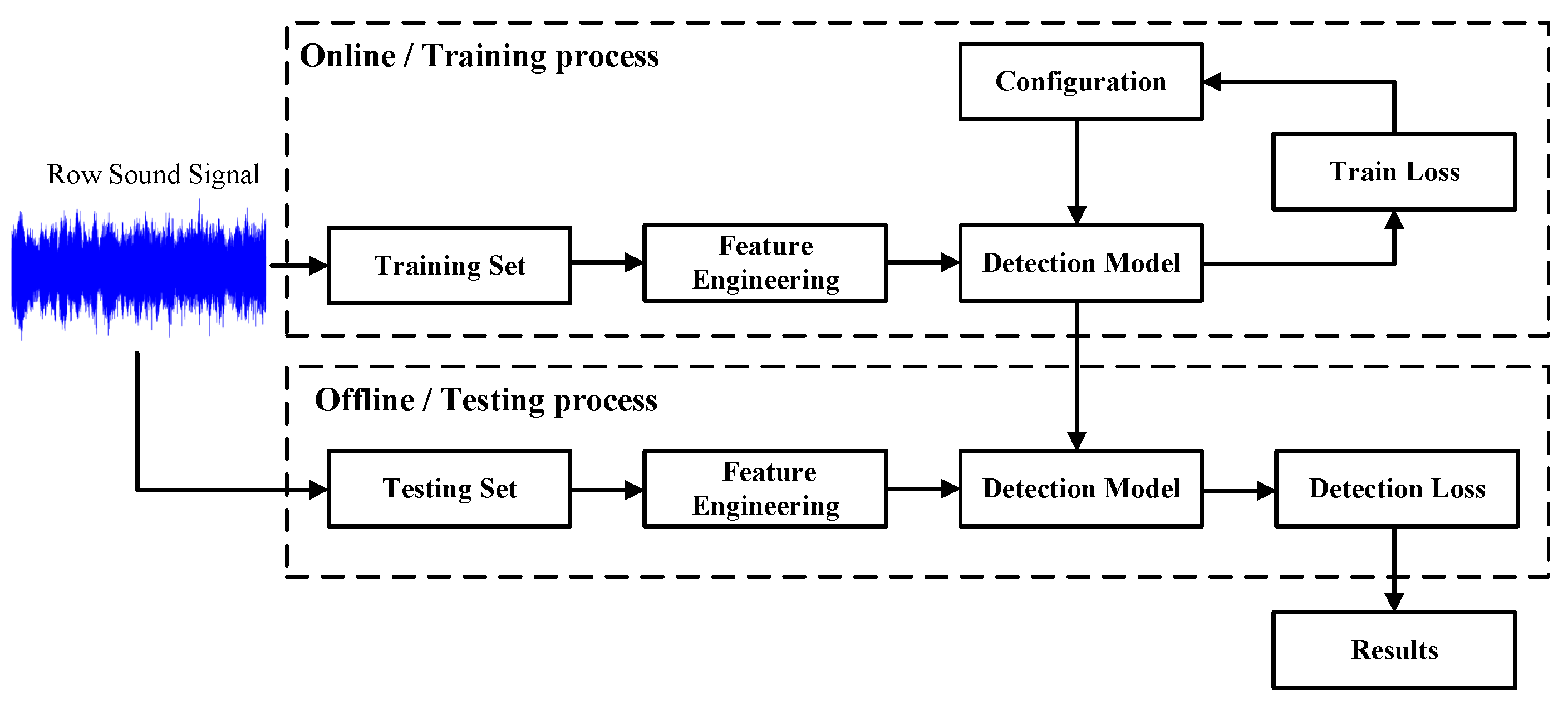
1. Introduction
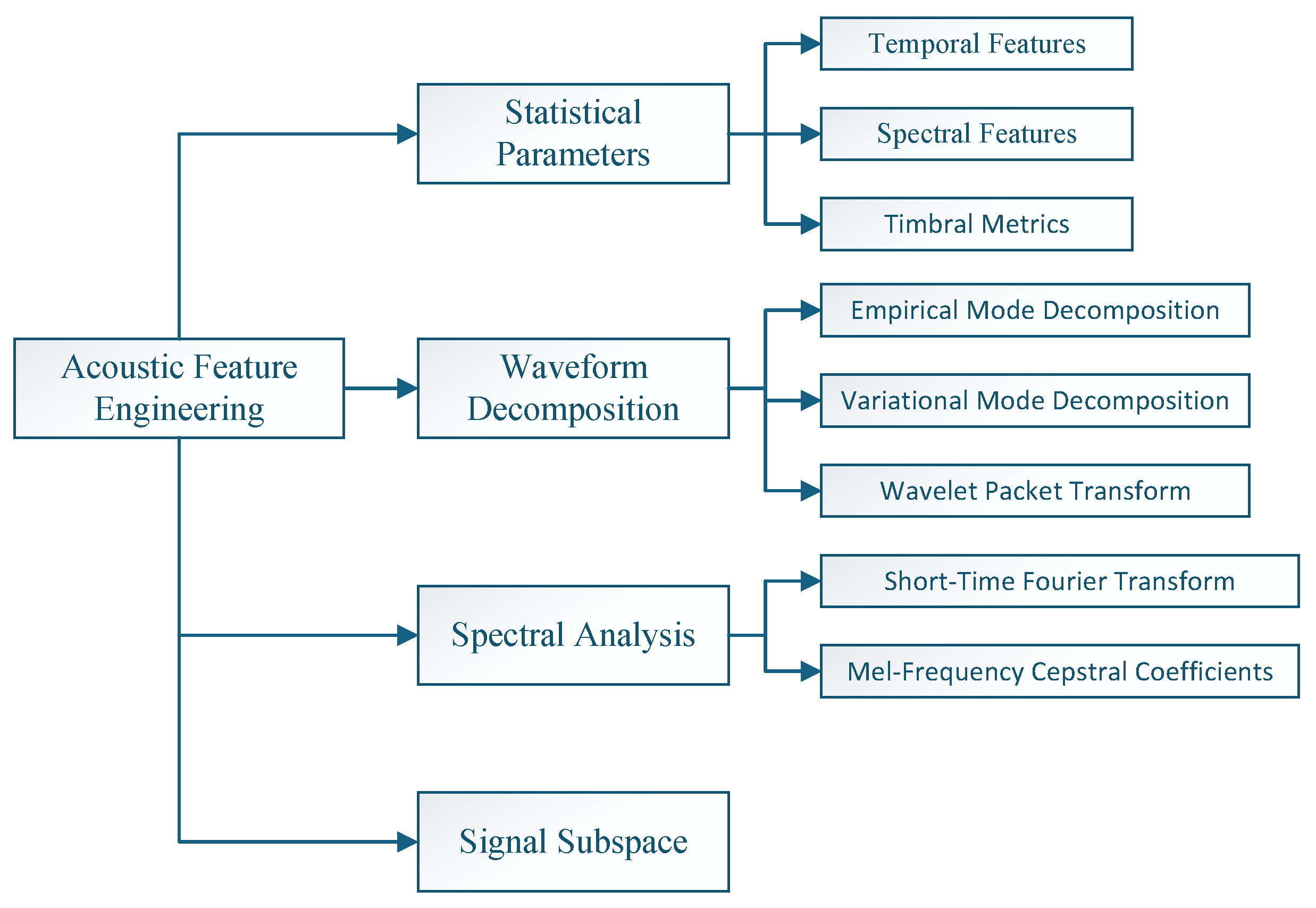
2. Acoustic Feature Engineering
2.1. Statistical Parameters
2.2. Waveform Decomposition
2.2.1. Empirical Mode Decomposition
2.2.2. Variational Mode Decomposition
2.2.3. Wavelet Packet Transform

| Methods | Pros | Cons | Ref. |
|---|---|---|---|
| EMD | Adaptive decomposition | Severe mode mixing issues. | [27,59] |
| without basis functions. | Highly sensitive to noise. | ||
| Suitable for non-stationary. | |||
| CEEMD | Suppresses mode mixing | Doubled computational complexity | [60] |
| Better detail preservation | Requires manual noise amplitude selection | ||
| EEMD | Reduces mode mixing through | Ensemble size requires empirical selection. | [73] |
| noise-assisted decomposition. | Influenced by the type of noise introduced. | ||
| Anti-noise Interference. | |||
| More reproducible and consistent. | |||
| VMD | Variational framework | Requires preset mode number K | [34,35,65] |
| ensures unique decomposition | |||
| WF-VMD | Wiener-filtered enhancement | Latency Per Frame | [65] |
| COA-VMD | Auto-optimizes K and | Increased computation time for optimization | [66] |
| SSA-VMD | Effective for multi-fault coexistence detection | Requires large iterations | [42] |
| WT | Flexible basis function selection | Energy leakage | [19,68] |
| DWT | Efficient implementation with filter banks | Limited shift-invariance | [31] |
| WPT + TEO | Quickly capture the resonant frequency | Manual threshold setting | [26] |
| bands of fault characteristics. |
2.3. Spectrogram Analysis
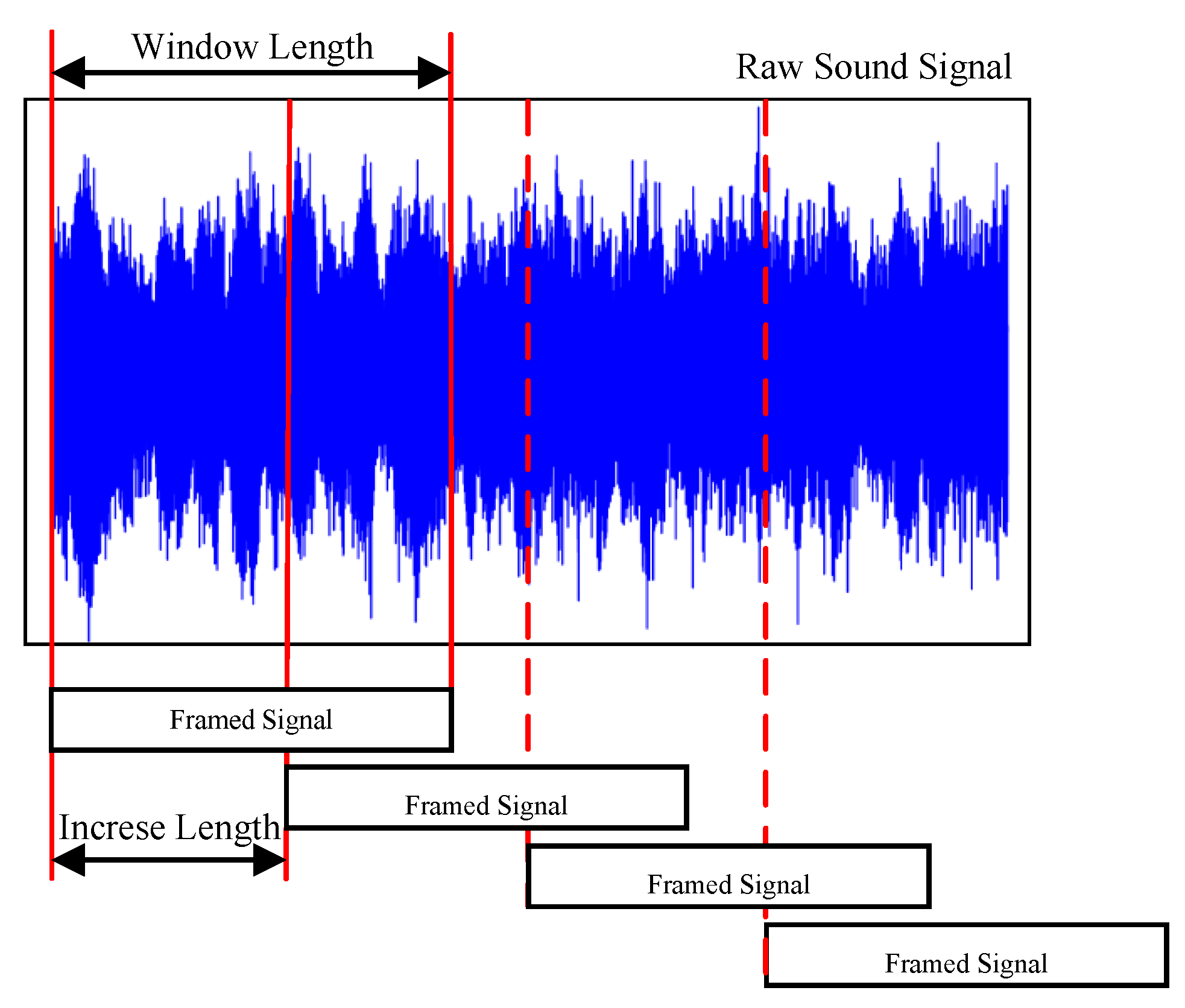
2.3.1. Short-Time Fourier Transform
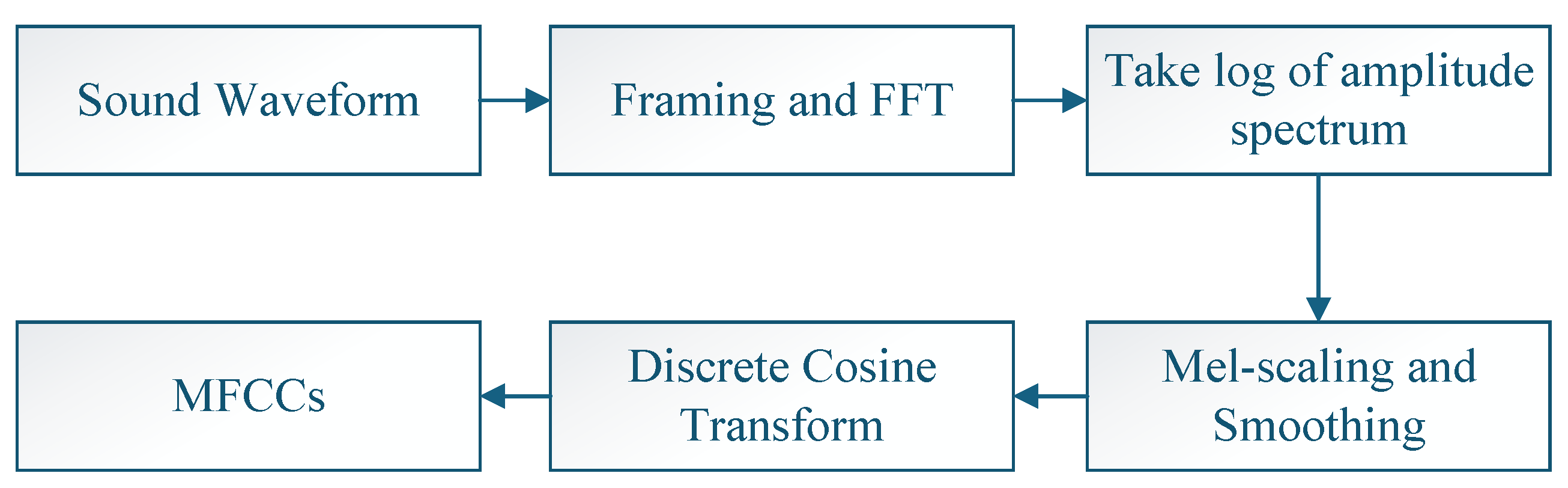
2.3.2. Mel-Frequency Cepstral Coefficient
| Sample Rate | Window Function | Window Length | Increase Length | Applications | Ref. |
|---|---|---|---|---|---|
| 8820 | Hanning | 819 | 205 | Multiple-equipment Recognition | [36] |
| 1920 | Hamming | 1920 | 960 | Underground Pipeline Damage | [41] |
| 256 | Hanning | 4096 | 2048 | Excavation Equipment | [81] |
| 1024 | - | 1024 | 512 | DCASE 2020 Task 2 | [45] |
| 2048 | Hamming | 2048 | 512 | Rotating Machinery | [33] |
2.4. Signal Subspace
3. Anomalous Sound Detection
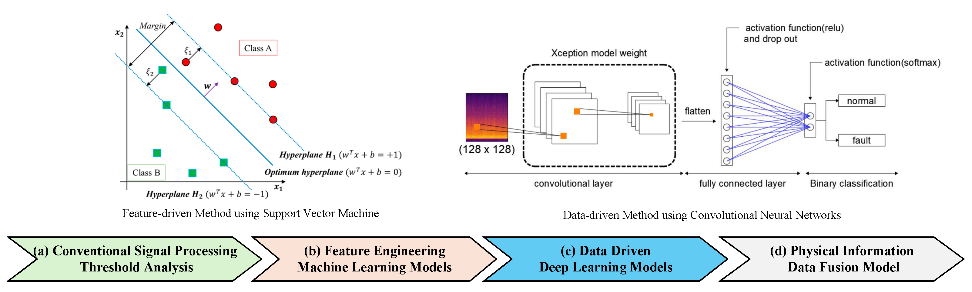
3.1. Experience-Driven Thresholding Analysis
3.2. Feature-Driven Machine Learning
3.3. Data-Driven Deep Learning
3.3.1. Image-Based Deep Learning
3.3.2. Sequence-Based Deep Learning
3.3.3. Graph-Based Deep Learning
4. Opportunities
5. Conclusions
Author Contributions
Funding
Data Availability Statement
Conflicts of Interest
Abbreviations
| PdM | Predictive Maintenance |
| SVM | Support Vector Machine |
| CNN | Convolutional Neural Network |
| WT | Wavelet Transform |
| MFCC | Mel-Frequency Cepstral Coefficient |
| HMM | Hidden Markov Model |
| DT | Decision Tree |
| DCNN | Deep Convolutional Neural Network |
| KNN | K-Nearest Neighbor |
| DWT | Discrete Wavelet Transform |
| STFT | Short-Time Fourier Transform |
| VMD | Variational Mode Decomposition |
| EMD | Empirical Mode Decomposition |
| AE | AutoEncoder |
| RF | Random Forest |
| LDA | Linear Discriminant Analysis |
| WPT | Wavelet Packet Transform |
| BiLSTM | Bi-directional Long Short-Term |
| BiGRU | Bidirectional Gated Recurrent Unit |
| DGCN | Deep Graph Convolutional Network |
| LSTM | Long Short-Term Memory |
| ANN | Artificial Neural Network |
| MLP | Multilayer Perceptron |
| BiTCN | Bi-directional Temporal Convolutional Network |
| TDGCN | Unsuper-Transformer and Dynamic Graph Convolution |
| GMM | Gaussian Mixture Model |
| FFT | Fast Fourier Transform |
| STE | Short-Time Energy |
| ZCR | Zero-Crossing Rate |
| IMF | Intrinsic Mode Function |
| CEEMD | Complete Ensemble Empirical Mode Decomposition |
| COA | Coati Optimization Algorithm |
| SSA | Sparrow Search Algorithm |
| WPA | Wavelet Packet Analysis |
| TEO | Teager Energy Operator |
| SC | Spectral Centroid |
| TR | Tonnetz representation |
| PCA | Principal Component Analysis |
| TESK | Teager Energy Spectral Kurtosis |
| TSFDR-LDA | Time-spectral features extraction |
| and reduction with linear discriminant analysis | |
| YAMNet | Yet Another Audio Mobilenet Network |
| DSN | Domain Self-adaptive Network |
| GAN | Generative Adversarial Network |
| PINN | Physics-informed Neural Network |
References
- Mennilli, R.; Mazza, L.; Mura, A. Integrating Machine Learning for Predictive Maintenance on Resource-Constrained PLCs: A Feasibility Study. Sensors 2025, 25, 537. [Google Scholar] [CrossRef] [PubMed]
- Zhang, W.; Yang, D.; Wang, H. Data-Driven Methods for Predictive Maintenance of Industrial Equipment: A Survey. IEEE Syst. J. 2019, 13, 2213–2227. [Google Scholar] [CrossRef]
- Tiago, Z.; Cristiano, A.D.; Rodrigo, D.; Miromar, J.d.; Eduardo, S.D.; Guann Pyng, L. Predictive maintenance in the Industry 4.0: A systematic literature review. Comput. Ind. Eng. 2020, 150, 106889. [Google Scholar]
- Pech, M.; Vrchota, J.; Bednář, J. Predictive maintenance and intelligent sensors in smart factory. Sensors 2021, 21, 1470. [Google Scholar] [CrossRef]
- Chan, T.K.; Chin, C.S. A Comprehensive Review of Polyphonic Sound Event Detection. IEEE Access 2020, 8, 103339–103373. [Google Scholar] [CrossRef]
- Amrit, S.; Chiranjeev, K.; Preetam, S. Early detection of mechanical malfunctions in vehicles using sound signal processing. Appl. Acoust. 2022, 188, 108578. [Google Scholar]
- Rihi, A.; Baïna, S.; Mhada, F.Z.; El Bachari, E.; Tagemouati, H.; Guerboub, M.; Benzakour, I.; Baïna, K.; Abdelwahed, E.H. Innovative predictive maintenance for mining grinding mills: From LSTM-based vibration forecasting to pixel-based MFCC image and CNN. Int. J. Adv. Manuf. Technol. 2024, 135, 1271–1289. [Google Scholar] [CrossRef]
- Yousuf, M.; Alsuwian, T.; Amin, A.A.; Fareed, S.; Hamza, M. IoT-based health monitoring and fault detection of industrial AC induction motor for efficient predictive maintenance. Meas. Control 2024, 57, 1146–1160. [Google Scholar] [CrossRef]
- Yong-Cheol, L.; Moeid, S.; Abbas, R.; Hyun Woo, L. Evidence-driven sound detection for prenotification and identification of construction safety hazards and accidents. Autom. Constr. 2020, 113, 103127. [Google Scholar]
- An, Q.; Zang, J.; Zhang, Z.; Gao, L.; Wang, G.; Xue, C. Integrated Acoustic-Vibratory Sensor Inspired by the Ear Bones of Sea Turtles for Heart Sound Detection. IEEE Sens. J. 2024, 24, 15865–15874. [Google Scholar] [CrossRef]
- Xiong, W.; Xu, X.; Chen, L.; Yang, J. Sound-Based Construction Activity Monitoring with Deep Learning. Buildings 2022, 12, 1947. [Google Scholar] [CrossRef]
- Ye, T.; Peng, T.; Li, J. A sound frequency ridge positioning model oriented to mine equipment. J. Vib. Control 2024, 30, 3402–3413. [Google Scholar] [CrossRef]
- Saucedo-Espinosa, M.A.; Escalante, H.J.; Berrones, A. Detection of defective embedded bearings by sound analysis: A machine learning approach. J. Intell. Manuf. 2017, 28, 489–500. [Google Scholar] [CrossRef]
- Chen, Y.; Chang, R.; Guo, J. Emotion recognition of EEG signals based on the ensemble learning method: AdaBoost. Math. Probl. Eng. 2021, 2021, 8896062. [Google Scholar] [CrossRef]
- Srinivasan, R.; Tamzeed Islam, M.; Islam, B.; Wang, Z.; Sookoor, T.; Gnawali, O.; Nirjon, S. Preventive maintenance of centralized HVAC systems: Use of acoustic sensors, feature extraction, and unsupervised learning. In Proceedings of the Building Simulation 2017, San Francisco, CA, USA, 7–9 August 2017; Volume 15, pp. 2518–2524. [Google Scholar]
- Zhang, T.; Lee, Y.C.; Scarpiniti, M.; Uncini, A. A supervised machine learning-based sound identification for construction activity monitoring and performance evaluation. In Proceedings of the Construction Research Congress 2018, New Orleans, LA, USA, 2–4 April 2018; pp. 358–366. [Google Scholar]
- Lee, J.; Choi, H.; Park, D.; Chung, Y.; Kim, H.Y.; Yoon, S. Fault detection and diagnosis of railway point machines by sound analysis. Sensors 2016, 16, 549. [Google Scholar] [CrossRef] [PubMed]
- Jung, H.; Choi, S.; Lee, B. Rotor fault diagnosis method using CNN-Based transfer learning with 2D sound spectrogram analysis. Electronics 2023, 12, 480. [Google Scholar] [CrossRef]
- Bai, K.; Zhou, Y.; Cui, Z.; Bao, W.; Zhang, N.; Zhai, Y. HOG-SVM-Based Image Feature Classification Method for Sound Recognition of Power Equipments. Energies 2022, 15, 4449. [Google Scholar] [CrossRef]
- Yu, Z.; Wei, Y.; Niu, B.; Zhang, X. Automatic Condition Monitoring and Fault Diagnosis System for Power Transformers Based on Voiceprint Recognition. IEEE Trans. Instrum. Meas. 2024, 73, 1–11. [Google Scholar] [CrossRef]
- Ayhan, A.; Ferhat, Y.; Orhan, Y. A sound based method for fault detection with statistical feature extraction in UAV motors. Appl. Acoust. 2021, 183, 108325. [Google Scholar]
- Suawa, P.F.; Halbinger, A.; Jongmanns, M.; Reichenbach, M. Noise-Robust Machine Learning Models for Predictive Maintenance Applications. IEEE Sens. J. 2023, 23, 15081–15092. [Google Scholar] [CrossRef]
- Yaman, O. An automated faults classification method based on binary pattern and neighborhood component analysis using induction motor. Measurement 2021, 168, 108323. [Google Scholar] [CrossRef]
- Yun, H.; Kim, H.; Jeong, Y.H.; Jun, M.B. Autoencoder-based anomaly detection of industrial robot arm using stethoscope based internal sound sensor. J. Intell. Manuf. 2023, 34, 1427–1444. [Google Scholar] [CrossRef]
- Josué, P.C.; Jesús, A.F.D.; Froylán, C.S.; Luz, M.; David, I.I.Z. Bearing fault detection with vibration and acoustic signals: Comparison among different machine leaning classification methods. Eng. Fail. Anal. 2022, 139, 106515. [Google Scholar]
- Zhang, X.; Wan, S.; He, Y.; Wang, X.; Dou, L. Teager energy spectral kurtosis of wavelet packet transform and its application in locating the sound source of fault bearing of belt conveyor. Measurement 2021, 173, 108367. [Google Scholar] [CrossRef]
- Shi, H.; Li, Y.; Bai, X.; Zhang, K.; Sun, X. A two-stage sound-vibration signal fusion method for weak fault detection in rolling bearing systems. Mech. Syst. Signal Process. 2022, 172, 109012. [Google Scholar] [CrossRef]
- Alharbi, F.; Luo, S.; Zhao, S.; Yang, G.; Wheeler, C.; Chen, Z. Belt Conveyor Idlers Fault Detection Using Acoustic Analysis and Deep Learning Algorithm With the YAMNet Pretrained Network. IEEE Sens. J. 2024, 24, 31379–31394. [Google Scholar] [CrossRef]
- Zhang, D.; Stewart, E.; Entezami, M.; Roberts, C.; Yu, D. Intelligent acoustic-based fault diagnosis of roller bearings using a deep graph convolutional network. Measurement 2020, 156, 107585. [Google Scholar] [CrossRef]
- Yan, H.; Bai, H.; Zhan, X.; Wu, Z.; Wen, L.; Jia, X. Combination of VMD mapping MFCC and LSTM: A new acoustic fault diagnosis method of diesel engine. Sensors 2022, 22, 8325. [Google Scholar] [CrossRef]
- Wang, Y.; Liu, N.; Guo, H.; Wang, X. An engine-fault-diagnosis system based on sound intensity analysis and wavelet packet pre-processing neural network. Eng. Appl. Artif. Intell. 2020, 94, 103765. [Google Scholar] [CrossRef]
- Espinosa, R.; Ponce, H.; Gutiérrez, S. Click-event sound detection in automotive industry using machine/deep learning. Appl. Soft Comput. 2021, 108, 107465. [Google Scholar] [CrossRef]
- Liu, Y.; Chen, Y.; Li, X.; Zhou, X.; Wu, D. MPNet: A lightweight fault diagnosis network for rotating machinery. Measurement 2025, 239, 115498. [Google Scholar] [CrossRef]
- Luo, Y.; Wang, M.; Luo, L.; Liu, Z.; Zhao, J. Optimized LSTM-BiTCN parallel network model for anomalous sound detection in rotating machinery. Meas. Sci. Technol. 2025, 36, 046110. [Google Scholar] [CrossRef]
- Yin, X.; He, Q.; Zhang, H.; Qin, Z.; Zhang, B. Sound Based Fault Diagnosis Method Based on Variational Mode Decomposition and Support Vector Machine. Electronics 2022, 11, 2422. [Google Scholar] [CrossRef]
- Sherafat, B.; Rashidi, A.; Asgari, S. Sound-based multiple-equipment activity recognition using convolutional neural networks. Autom. Constr. 2022, 135, 104104. [Google Scholar] [CrossRef]
- Eleni, T.; Andreas, P.; Maria, S. Monitoring, profiling and classification of urban environmental noise using sound characteristics and the KNN algorithm. Energy Rep. 2020, 6, 223–230. [Google Scholar]
- Cao, Y.; Sun, Y.; Xie, G.; Li, P. A Sound-Based Fault Diagnosis Method for Railway Point Machines Based on Two-Stage Feature Selection Strategy and Ensemble Classifier. IEEE Trans. Intell. Transp. Syst. 2022, 23, 12074–12083. [Google Scholar] [CrossRef]
- Yan, J.; Cheng, Y.; Wang, Q.; Liu, L.; Zhang, W.; Jin, B. Transformer and Graph Convolution-Based Unsupervised Detection of Machine Anomalous Sound Under Domain Shifts. IEEE Trans. Emerg. Top. Comput. Intell. 2024, 8, 2827–2842. [Google Scholar] [CrossRef]
- Notani, K.; Hayashi, T.; Mori, N. Abnormal Sound Detection in Pipes Using a Wireless Microphone and Machine Learning. Mater. Trans. 2022, 63, 1622–1630. [Google Scholar] [CrossRef]
- Liu, Z.; Li, S. A sound monitoring system for prevention of underground pipeline damage caused by construction. Autom. Constr. 2020, 113, 103125. [Google Scholar] [CrossRef]
- Li, S.; Zhao, Q.; Liu, J.; Zhang, X.; Hou, J. Noise Reduction of Steam Trap Based on SSA-VMD Improved Wavelet Threshold Function. Sensors 2025, 25, 1573. [Google Scholar] [CrossRef]
- Kong, D.; Yu, H.; Yuan, G. Multi-Spectral and Multi-Temporal Features Fusion with SE Network for Anomalous Sound Detection. IEEE Access 2024, 12, 167262–167277. [Google Scholar] [CrossRef]
- Wu, J.; Yang, F.; Hu, W. Unsupervised anomalous sound detection for industrial monitoring based on ArcFace classifier and gaussian mixture model. Appl. Acoust. 2023, 203, 109188. [Google Scholar] [CrossRef]
- Liu, Y.; Guan, J.; Zhu, Q.; Wang, W. Anomalous Sound Detection Using Spectral-Temporal Information Fusion. In Proceedings of the ICASSP 2022—2022 IEEE International Conference on Acoustics, Speech and Signal Processing (ICASSP), Singapore, 22–27 May 2022; pp. 816–820. [Google Scholar]
- Kim, S.M.; Soo Kim, Y. Enhancing Sound-Based Anomaly Detection Using Deep Denoising Autoencoder. IEEE Access 2024, 12, 84323–84332. [Google Scholar] [CrossRef]
- Ota, Y.; Unoki, M. Anomalous Sound Detection for Industrial Machines Using Acoustical Features Related to Timbral Metrics. IEEE Access 2023, 11, 70884–70897. [Google Scholar] [CrossRef]
- Emanuele, D.; Antonino, F.; Antonio, G.; Vincenzo, M.; Giancarlo, S. An anomalous sound detection methodology for predictive maintenance. Expert Syst. Appl. 2022, 209, 118324. [Google Scholar]
- Ren, J.; Hu, C.; Shang, Z.; Li, Y.; Zhao, Z.; Yan, R. Learning Interpretable and Transferable Representations via Wavelet-constrained Transformer for Industrial Acoustic Diagnosis. IEEE Trans. Instrum. Meas. 2025, 74, 3512312. [Google Scholar] [CrossRef]
- Majasan, J.O.; Robinson, J.B.; Owen, R.E.; Maier, M.; Radhakrishnan, A.N.; Pham, M.; Tranter, T.G.; Zhang, Y.; Shearing, P.R.; Brett, D.J. Recent advances in acoustic diagnostics for electrochemical power systems. J. Phys. Energy 2021, 3, 032011. [Google Scholar] [CrossRef]
- Fang, H.; An, J.; Liu, H.; Xiang, J.; Zhao, B.; Dunkin, F. A lightweight transformer with strong robustness application in portable bearing fault diagnosis. IEEE Sens. J. 2023, 23, 9649–9657. [Google Scholar] [CrossRef]
- Suraj, G.; Akhilesh, K.; Jhareswar, M. A critical review on system architecture, techniques, trends and challenges in intelligent predictive maintenance. Saf. Sci. 2024, 177, 106590. [Google Scholar]
- Wang, X.; Mao, D.; Li, X. Bearing fault diagnosis based on vibro-acoustic data fusion and 1D-CNN network. Measurement 2021, 173, 108518. [Google Scholar] [CrossRef]
- Mian, T.; Choudhary, A.; Fatima, S. An efficient diagnosis approach for bearing faults using sound quality metrics. Appl. Acoust. 2022, 195, 108839. [Google Scholar] [CrossRef]
- Ono, Y.; Onishi, Y.; Koshinaka, T.; Takata, S.; Hoshuyama, O. Anomaly detection of motors with feature emphasis using only normal sounds. In Proceedings of the 2013 IEEE International Conference on Acoustics, Speech and Signal Processing, Vancouver, BC, Canada, 26–31 May 2013; pp. 2800–2804. [Google Scholar]
- Peng, Y.; Li, Z.; He, K.; Liu, Y.; Li, Q.; Liu, L. Broadband mode decomposition and its application to the quality evaluation of welding inverter power source signals. IEEE Trans. Ind. Electron. 2019, 67, 9734–9746. [Google Scholar] [CrossRef]
- Huang, N.E.; Shen, Z.; Long, S.R.; Wu, M.C.; Shih, H.H.; Zheng, Q.; Yen, N.C.; Tung, C.C.; Liu, H.H. The empirical mode decomposition and the Hilbert spectrum for nonlinear and non-stationary time series analysis. Proc. R. Soc. Lond. Ser. A Math. Phys. Eng. Sci. 1998, 454, 903–995. [Google Scholar] [CrossRef]
- Li, R.; He, D. Rotational machine health monitoring and fault detection using EMD-based acoustic emission feature quantification. IEEE Trans. Instrum. Meas. 2012, 61, 990–1001. [Google Scholar] [CrossRef]
- Amarnath, M. andPraveen Krishna, I. Local fault detection in helical gears via vibration and acoustic signals using EMD based statistical parameter analysis. Measurement 2014, 58, 154–164. [Google Scholar] [CrossRef]
- Delgado-Arredondo, P.A.; Morinigo-Sotelo, D.; Osornio-Rios, R.A.; Avina-Cervantes, J.G.; Rostro-Gonzalez, H.; de Jesus Romero-Troncoso, R. Methodology for fault detection in induction motors via sound and vibration signals. Mech. Syst. Signal Process. 2017, 83, 568–589. [Google Scholar] [CrossRef]
- Torres, M.E.; Colominas, M.A.; Schlotthauer, G.; Flandrin, P. A complete ensemble empirical mode decomposition with adaptive noise. In Proceedings of the 2011 IEEE International Conference on Acoustics, Speech and Signal Processing (ICASSP), Prague, Czech Republic, 22–27 May 2011; pp. 4144–4147. [Google Scholar]
- Gai, J.; Shen, J.; Hu, Y.; Wang, H. An integrated method based on hybrid grey wolf optimizer improved variational mode decomposition and deep neural network for fault diagnosis of rolling bearing. Measurement 2020, 162, 107901. [Google Scholar] [CrossRef]
- Chen, B.; Zhang, W.; James, X.; Song, D.; Cheng, Y.; Zhou, Z.; Gu, F.; Andrew, D.B. Product envelope spectrum optimization-gram: An enhanced envelope analysis for rolling bearing fault diagnosis. Mech. Syst. Signal Process. 2023, 193, 110270. [Google Scholar] [CrossRef]
- Xu, B.; Zhou, F.; Li, H.; Yan, B.; Liu, Y. Early fault feature extraction of bearings based on Teager energy operator and optimal VMD. ISA Trans. 2019, 86, 249–265. [Google Scholar] [CrossRef]
- Xiao, Y.; Feng, X.; Lv, J.; Shen, Y.; Zhou, S.; Zhou, N.; Du, Z. Sealing strip acoustic performance evaluation using WF-VMD based signal enhancement method. Appl. Acoust. 2024, 217, 109860. [Google Scholar] [CrossRef]
- Lei, W.; Guo, W.; Wan, B.; Min, Y.; Wu, J.; Li, B. High voltage shunt reactor acoustic signal denoising based on the combination of VMD parameters optimized by coati optimization algorithm and wavelet threshold. Measurement 2024, 224, 113854. [Google Scholar] [CrossRef]
- Gharehchopogh, F.S.; Namazi, M.; Ebrahimi, L.; Abdollahzadeh, B. Advances in sparrow search algorithm: A comprehensive survey. Arch. Comput. Methods Eng. 2023, 30, 427–455. [Google Scholar] [CrossRef]
- Chen, L.J.; Lin, W.M.; Tsao, T.P.; Lin, Y.H. Study of Partial Discharge Measurement in Power Equipment Using Acoustic Technique and Wavelet Transform. IEEE Trans. Power Deliv. 2007, 22, 1575–1580. [Google Scholar] [CrossRef]
- Lou, X.; Loparo, A.K. Bearing fault diagnosis based on wavelet transform and fuzzy inference. Mech. Syst. Signal Process. 2004, 18, 1077–1095. [Google Scholar] [CrossRef]
- Wang, Y. Sound quality estimation for nonstationary vehicle noises based on discrete wavelet transform. J. Sound Vib. 2009, 324, 1124–1140. [Google Scholar] [CrossRef]
- Vonesch, C.; Blu, T.; Unser, M. Generalized Daubechies wavelet families. IEEE Trans. Signal Process. 2007, 55, 4415–4429. [Google Scholar] [CrossRef]
- Bozchalooi, I.S.; Liang, M. Teager energy operator for multi-modulation extraction and its application for gearbox fault detection. Smart Mater. Struct. 2010, 19, 075008. [Google Scholar] [CrossRef]
- Yang, Z.X.; Zhong, J.H. A hybrid EEMD-based SampEn and SVD for acoustic signal processing and fault diagnosis. Entropy 2016, 18, 112. [Google Scholar] [CrossRef]
- Jung, S.Y.; Liao, C.H.; Wu, Y.S.; Yuan, S.M.; Sun, C.T. Efficiently classifying lung sounds through depthwise separable CNN models with fused STFT and MFCC features. Diagnostics 2021, 11, 732. [Google Scholar] [CrossRef]
- Ramalingam, A.; Krishnan, S. Gaussian mixture modeling of short-time Fourier transform features for audio fingerprinting. IEEE Trans. Inf. Forensics Secur. 2006, 1, 457–463. [Google Scholar] [CrossRef]
- He, M.; He, D. Deep Learning Based Approach for Bearing Fault Diagnosis. IEEE Trans. Ind. Appl. 2017, 53, 3057–3065. [Google Scholar] [CrossRef]
- Singh, M.K.; Kumar, S.; Nandan, D. Faulty voice diagnosis of automotive gearbox based on acoustic feature extraction and classification technique. J. Eng. Res. 2023, 11, 100051. [Google Scholar] [CrossRef]
- Liu, X.; Pei, D.; Lodewijks, G.; Zhao, Z.; Mei, J. Acoustic signal based fault detection on belt conveyor idlers using machine learning. Adv. Powder Technol. 2020, 31, 2689–2698. [Google Scholar] [CrossRef]
- Le, P.N.; Ambikairajah, E.; Epps, J.; Sethu, V.; Choi, E.H. Investigation of spectral centroid features for cognitive load classification. Speech Commun. 2011, 53, 540–551. [Google Scholar] [CrossRef]
- Harte, C.; Sandler, M.; Gasser, M. Detecting harmonic change in musical audio. In Proceedings of the 1st ACM Workshop on Audio and Music Computing Multimedia, Santa Barbara, CA, USA, 23–27 October 2006; pp. 21–26. [Google Scholar]
- Cao, J.; Huang, W.; Zhao, T.; Wang, J.; Wang, R. An enhance excavation equipments classification algorithm based on acoustic spectrum dynamic feature. Multidimens. Syst. Signal Process. 2017, 28, 921–943. [Google Scholar] [CrossRef]
- Yadav, S.K.; Tyagi, K.; Shah, B.; Kalra, P.K. Audio Signature-Based Condition Monitoring of Internal Combustion Engine Using FFT and Correlation Approach. IEEE Trans. Instrum. Meas. 2011, 60, 1217–1226. [Google Scholar] [CrossRef]
- Sarradj, E. A fast signal subspace approach for the determination of absolute levels from phased microphone array measurements. J. Sound Vib. 2010, 329, 1553–1569. [Google Scholar] [CrossRef]
- Mahyub, M.; Souza, L.S.; Batalo, B.; Fukui, K. Signal latent subspace: A new representation for environmental sound classification. Appl. Acoust. 2024, 225, 110181. [Google Scholar] [CrossRef]
- Lawal, A.; Iqbal, N.; Zerguine, A.; Noui-Mehidi, M.N.; Zeghlache, M.L.; Al-Shaikhi, A.A. A Novel PCA-Based Slug Flow Characterization Using Acoustic Sensing. IEEE Access 2024, 12, 42849–42859. [Google Scholar] [CrossRef]
- Rabiner, L.R. A tutorial on hidden Markov models and selected applications in speech recognition. Proc. IEEE 1989, 77, 257–286. [Google Scholar] [CrossRef]
- Lang, R.; Lu, R.; Zhao, C.; Qin, H.; Liu, G. Graph-based semi-supervised one class support vector machine for detecting abnormal lung sounds. Appl. Math. Comput. 2020, 364, 124487. [Google Scholar] [CrossRef]
- Sack, S.; Åbom, M. Acoustic plane-wave decomposition by means of multilayer perceptron neural networks. J. Sound Vib. 2020, 486, 115518. [Google Scholar] [CrossRef]
- Sabillon, C.A.; Rashidi, A.; Samanta, B.; Cheng, C.F.; Davenport, M.A.; Anderson, D.V. A productivity forecasting system for construction cyclic operations using audio signals and a Bayesian approach. In Proceedings of the Construction Research Congress 2018, New Orleans, LA, USA, 2–4 April 2018; pp. 295–304. [Google Scholar]
- Sun, Z.; Tao, W.; Gao, M.; Zhang, M.; Song, S.; Wang, G. Broiler health monitoring technology based on sound features and random forest. Eng. Appl. Artif. Intell. 2024, 135, 108849. [Google Scholar] [CrossRef]
- Yin, X.; He, Q.; Peng, S.; Zhang, Y.; Zhang, B. A Fault Diagnosis Method Based on EMD-SVM with Multi-Feature Fusion via Sound Signals. In Proceedings of the 2022 IEEE International Conference on Real-time Computing and Robotics (RCAR), Guiyang, China, 17–22 July 2022; pp. 540–544. [Google Scholar]
- Grossberg, S. Nonlinear neural networks: Principles, mechanisms, and architectures. Neural Netw. 1988, 1, 17–61. [Google Scholar] [CrossRef]
- Koizumi, Y.; Saito, S.; Uematsu, H.; Kawachi, Y.; Harada, N. Unsupervised Detection of Anomalous Sound Based on Deep Learning and the Neyman–Pearson Lemma. IEEE/ACM Trans. Audio Speech Lang. Process. 2019, 27, 212–224. [Google Scholar] [CrossRef]
- Koizumi, Y.; Saito, S.; Uematsu, H.; Harada, N. Optimizing acoustic feature extractor for anomalous sound detection based on Neyman-Pearson lemma. In Proceedings of the 2017 25th European Signal Processing Conference (EUSIPCO), Kos Island, Greece, 28 August–2 September 2017; pp. 698–702. [Google Scholar]
- Yun, E.; Jeong, M. Acoustic Feature Extraction and Classification Techniques for Anomaly Sound Detection in the Electronic Motor of Automotive EPS. IEEE Access 2024, 12, 149288–149307. [Google Scholar] [CrossRef]
- Ruff, L.; Kauffmann, J.R.; Vandermeulen, R.A.; Montavon, G.; Samek, W.; Kloft, M.; Dietterich, T.G.; Müller, K.R. A Unifying Review of Deep and Shallow Anomaly Detection. Proc. IEEE 2021, 109, 756–795. [Google Scholar] [CrossRef]
- Park, Y.; Yun, I.D. Fast Adaptive RNN Encoder–Decoder for Anomaly Detection in SMD Assembly Machine. Sensors 2018, 18, 3573. [Google Scholar] [CrossRef]
- Deng, J.; Guo, J.; Xue, N.; Zafeiriou, S. ArcFace: Additive Angular Margin Loss for Deep Face Recognition. In Proceedings of the 2019 IEEE/CVF Conference on Computer Vision and Pattern Recognition (CVPR), Long Beach, CA, USA, 15–20 June 2019; pp. 4685–4694. [Google Scholar]
- Chen, S.; Liu, Y.; Gao, X.; Han, Z. Mobilefacenets: Efficient cnns for accurate real-time face verification on mobile devices. In Proceedings of the Chinese Conference on Biometric Recognition, Urumqi, China, 11–12 August 2018; pp. 428–438. [Google Scholar]
- Van Den Oord, A.; Dieleman, S.; Zen, H.; Simonyan, K.; Vinyals, O.; Graves, A.; Kalchbrenner, N.; Senior, A.; Kavukcuoglu, K. Wavenet: A generative model for raw audio. arXiv 2016, arXiv:1609.03499. [Google Scholar]
- Cheng, T.; Guo, F. Machine anomalous sound detection based on audio synthesis generative adversarial network. J. Phys. Conf. Ser. 2024, 2816, 012041. [Google Scholar] [CrossRef]
- Purohit, H.; Tanabe, R.; Ichige, K.; Endo, T.; Nikaido, Y.; Suefusa, K.; Kawaguchi, Y. MIMII Dataset: Sound dataset for malfunctioning industrial machine investigation and inspection. arXiv 2019, arXiv:1909.09347. [Google Scholar]
- Jiang, Y.; Dai, P.; Fang, P.; Zhong, R.Y.; Cao, X. Electrical-STGCN: An electrical spatio-temporal graph convolutional network for intelligent predictive maintenance. IEEE Trans. Ind. Inform. 2022, 18, 8509–8518. [Google Scholar] [CrossRef]
- Madhu, A.; K, S. EnvGAN: A GAN-based augmentation to improve environmental sound classification. Artif. Intell. Rev. 2022, 55, 6301–6320. [Google Scholar] [CrossRef]
- Premachandra, C.; Kunisada, Y. GAN Based Audio Noise Suppression for Victim Detection at Disaster Sites with UAV. IEEE Trans. Serv. Comput. 2024, 17, 183–193. [Google Scholar] [CrossRef]
- Olivieri, M.; Karakonstantis, X.; Pezzoli, M.; Antonacci, F.; Sarti, A.; Fernandez-Grande, E. Physics-informed neural network for volumetric sound field reconstruction of speech signals. EURASIP J. Audio Speech Music Process. 2024, 2024, 42. [Google Scholar] [CrossRef]
- Koyama, S.; Ribeiro, J.G.; Nakamura, T.; Ueno, N.; Pezzoli, M. Physics-Informed Machine Learning for Sound Field Estimation: Fundamentals, state of the art, and challenges [Special Issue on Model-Based and Data-Driven Audio Signal Processing]. IEEE Signal Process. Mag. 2025, 41, 60–71. [Google Scholar] [CrossRef]


| Applications | Feature Engineering | Detection Methods | Accuracy | Ref. |
|---|---|---|---|---|
| Power System | Wavelet Transform (WT) + Histogram of Oriented Gradient | Support Vector Machine (SVM) | 90% | [19] |
| Statistical Features Mel-Frequency Cepstral Coefficients (MFCCs) | Experience Thresholds Hidden Markov Model (HMM) | 97.83% | [20] | |
| Motor | Statistical Features | Decision Tree (DT) + SVM + K-Nearest Neighbor (KNN) | 99.75% | [21] |
| Raw Waveform | Deep Convolutional Neural Networks (DCNNs) | 95% | [22] | |
| Discrete Wavelet Transform (DWT) | SVM + KNN | 92.12% | [23] | |
| Short-Time Fourier Transform (STFT) | AutoEncoder (AE) | 96.4% | [24] | |
| Bearing | Statistical Features DWT Time-Spectral Features | SVM Random Forest (RF) Linear Discriminant Analysis (LDA) | 96.78% 96.79% 95.60% | [25] |
| Wavelet Packet Transform (WPT) + Teager Energy Operator | Kurtosis Index | - | [26] | |
| Empirical Mode Decomposition (EMD) + Kurtosis Superposition | Appropriate Threshold | - | [27] | |
| Raw Waveform | Convolutional Natural Network (CNN) + Bi-directional Long Short-Term Memory (BiLSTM) + Bidirectional Gated Recurrent Unit (BiGRU) | 90% | [28] | |
| Raw Waveform | Deep Graph Convolutional Networks (DGCN) | 91% | [29] | |
| Engine | Variational Mode Decomposition (VMD) + MFCC | Long Short-Term Memory (LSTM) | 97% | [30] |
| DWT + WPT | Artificial Neural Network (ANN) | 90% | [31] | |
| MFCC | Multilayer Perceptron (MLP) + CNN | 94.55% | [32] | |
| Rotating machinery | STFT | MPNet | 95.83% | [33] |
| STFT + VMD | LSTM + Bi-directional Temporal Convolutional Network (BiTCN) | 94.1% | [34] | |
| Car Mirror Folding | VMD + Statistical Features | SVM | 95.8% | [35] |
| Equipment | STFT | CNN | 82.8% | [36] |
| Environments | Statistical Features + MFCC | KNN | 85% | [37] |
| Railway Machines | EMD + Statistical Features | Weighted Majority Voting | 99% | [38] |
| Home Appliance | STFT | Unsuper-Transformer and Dynamic Graph Convolution (TDGCN) | 99.23% | [39] |
| Pipes | Principal Component Analysis | One Class-SVM | 100% | [40] |
| Statistical Features + MFCC | RF | 95.59% | [41] | |
| Sparrow Search Algorithm-VMD | Wavelet Thresholding | - | [42] | |
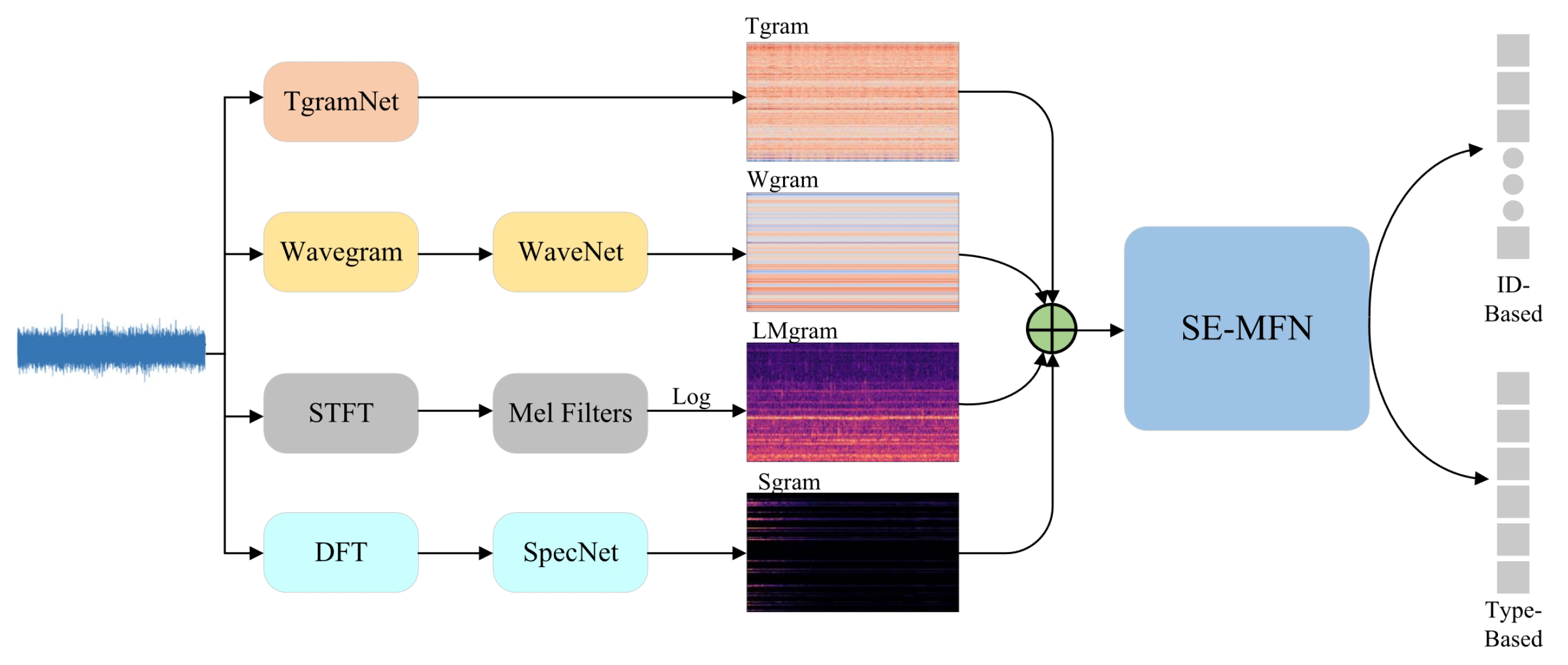
| DCASE 2020 Task 2 | Raw Waveform + MFCC | TgramNet + WaveNet + SpecNet + MobileFaceNet | 95.97% | [43] |
| STFT | CNN + Gaussian Mixture Model (GMM) | 96.86% | [44] | |
| Raw Waveform + MFCC | STgram + MFN | 92.36% | [45] | |
| MIMII | MFCC + Statistical Features | Deep Denoising Autoencoder | 96.51% | [46] |
| Timbral Features | SVM | 97% | [47] | |
| STFT + MFCC + ID | LSTM-AE | 84.14% | [48] |
| Classification | Feature Names | Equations |
|---|---|---|
| Temporal | Short-Time Energy | |
| Zero-Crossing Rate | ||
| Root Mean Square | ||
| The -order moment | ||
| Standard Deviation | ||
| Kurtosis | ||
| Skewness | ||
| Peak | ||
| Peak-to-Peak | ||
| Crest Factor | ||
| Impulse Factor | ||
| Margin Factor | ||
| Talaf | ||
| Tikhat | ||
| Spectral | Fast Fourier Transform (FFT) | |
| Peak | ||
| Peak Frequency | ||
| Mean Frequency | ||
| Frequency Center | ||
| RMS Frequency | ||
| Standard Deviation | ||
| Frequency Power Envelop | ||
| Effective Value | ||
| Envelop Amplitudes | ||
| Median Frequency | ||
| Relative Peak | ||
| Timbral Metrics | Sharpness | |
| Roughness | ||
| Boominess | ||
| Brightness | ||
| Depth |
| Features Extraction Method | Feature Dimensions | Ref. | |||
|---|---|---|---|---|---|
| Statistical Parameters | Decomposition | Spectrogram | |||
| Temporal | Spectral | ||||
| Short-time Energy Zero-crossing Rate | - | - | 12-level MFCC | [20] | |
| Mean | Mean Frequency | 15-level EMD | - | [38] | |
| Standard Deviation | Frequency Center | 8-level WPD | |||
| Skewness | RMS Frequency | ||||
| Kurtosis | Standard Deviation | ||||
| Peak | Energy Entropy | ||||
| RMS | |||||
| Crest Factor | |||||
| Shape Factor | |||||
| Impulse Factor | |||||
| Margin Factor | |||||
| RMS | RMS Frequency | 8-level DWT | - | [25] | |
| Kurtosis | Mean Frequency | ||||
| Peak to Peak | Frequency Power Envelop | ||||
| Crest Factor | Effective Value | ||||
| Skewness | Envelop Amplitudes | ||||
| Impulse Factor | |||||
| Standard Deviation | |||||
| Talaf | |||||
| Tikhat | |||||
| RMS | Peak | - | MFCC | [40] | |
| Crest Factor | Peak Frequency | ||||
| Median Frequency | |||||
| Relative Peak | |||||
| RMS | Spectral Envelope | - | mass center | [37] | |
| Standard Deviation | Centroid | peak amplitude | |||
| Skewness | Skewness | ||||
| Zero-crossing Rate | |||||
| Crest Factor | |||||
| Kurtosis | |||||
| Spread | |||||
| Decrease | |||||
| Sharpness | - | - | [47] | ||
| Roughness | |||||
| Boominess | |||||
| Brightness | |||||
| Depth | |||||
| Types | Model | Loss Function | Pros | Cons | Ref. |
|---|---|---|---|---|---|
| Image | MPNet | Cross-Entropy | Lightweight | Weak Generalizability | [33] |
| Embedded Deployment | Speed Needs Improving | ||||
| CNN + GMM | Arcface | High stability | Unsteady signals inefficient | [44] | |
| STgram + MFN | Arcface | spectral temporal fusion | - | [45] | |
| SE-MFN | Arcface | Multi-feature fusion | Limitations real time | [43] | |
| Classification + ID | |||||
| CNN | Cross-Entropy | Better resource allocation | Scene limitations | [36] | |
| DNN | - | Noise robustness | Dependent noise samples | [22] | |
| Sequence | DDAE | Squared Error | Rapid processing speed | Noise Interference | [46] |
| FARED | Euclidean distance | fast adaptation | huge storage resources | [97] | |
| long training time | |||||
| LSTM | cross-entropy | Quickly Judge | Dependent trained samples | [30] | |
| ID-CN + LSTM + AE | ID loss | noise reduction | Scenario limitations | [48] | |
| BiLSTM + BiGRUs | Binary cross-entropy | high accuracy | Dataset limitations | [28] | |
| Computational efficiency | High model complexity | ||||
| LSTM + BiTCN | Binary Cross-Entropy | Efficient feature integration | generalization Limitations | [34] | |
| Graph | DGCN | Cross-Entropy | Information Richness | Graph Construction | [39] |
| Dependencies | |||||
| Unsuper-TDGCN | Fusion Loss | Domain Adaptation | Parameter Sensitivity | [29] | |
| Efficiency and Robustness | Real-World Validation |
| Equipment | Environments | Feature Engineering | Applications |
|---|---|---|---|
| Constant Power | Low Noise | Statistical Parameters | Power System |
| High Noise | EMD, MFCC | Motor, bearing, Railway | |
| Variable Power | Low Noise | VMD, DWT | Engine |
| High Noise | STFT, Signal Subspace | Rotating Machines |
Disclaimer/Publisher’s Note: The statements, opinions and data contained in all publications are solely those of the individual author(s) and contributor(s) and not of MDPI and/or the editor(s). MDPI and/or the editor(s) disclaim responsibility for any injury to people or property resulting from any ideas, methods, instructions or products referred to in the content. |
© 2025 by the authors. Licensee MDPI, Basel, Switzerland. This article is an open access article distributed under the terms and conditions of the Creative Commons Attribution (CC BY) license (https://creativecommons.org/licenses/by/4.0/).
Share and Cite
Ye, T.; Peng, T.; Yang, L. Review on Sound-Based Industrial Predictive Maintenance: From Feature Engineering to Deep Learning. Mathematics 2025, 13, 1724. https://doi.org/10.3390/math13111724
Ye T, Peng T, Yang L. Review on Sound-Based Industrial Predictive Maintenance: From Feature Engineering to Deep Learning. Mathematics. 2025; 13(11):1724. https://doi.org/10.3390/math13111724
Chicago/Turabian StyleYe, Tongzhou, Tianhao Peng, and Lidong Yang. 2025. "Review on Sound-Based Industrial Predictive Maintenance: From Feature Engineering to Deep Learning" Mathematics 13, no. 11: 1724. https://doi.org/10.3390/math13111724
APA StyleYe, T., Peng, T., & Yang, L. (2025). Review on Sound-Based Industrial Predictive Maintenance: From Feature Engineering to Deep Learning. Mathematics, 13(11), 1724. https://doi.org/10.3390/math13111724