Article

Stiffness Regulation of Cable-Driven Redundant Manipulators Through Combined Optimization of Configuration and Cable Tension

by
Zhuo Liang
1,
Pengkun Quan
2 and
Shichun Di
1,*
1
School of Mechatronics Engineering, Harbin Institute of Technology, Harbin 150001, China
2
School of Mechatronics Engineering, Henan University of Science and Technology, Luoyang 471003, China
*
Author to whom correspondence should be addressed.
Mathematics 2025, 13(11), 1714; https://doi.org/10.3390/math13111714
Submission received: 4 April 2025 / Revised: 15 May 2025 / Accepted: 22 May 2025 / Published: 23 May 2025

Abstract

Cable-driven redundant manipulators (CDRMs) are widely applied in various fields due to their notable advantages. Stiffness regulation capability is essential for CDRMs, as it enhances their adaptability and stability in diverse task scenarios. However, their stiffness regulation still faces two main challenges. First, stiffness regulation methods that involve physical structural modifications increase system complexity and reduce flexibility. Second, methods that rely solely on cable tension are constrained by the inherent stiffness of the cables, limiting the achievable regulation range. To address these challenges, this paper proposes a novel stiffness regulation method for CDRMs through the combined optimization of configuration and cable tension. A stiffness model is established to analyze the influence of the configuration and cable tension on stiffness. Due to the redundancy in degrees of freedom (DOFs) and actuation cables, there exist infinitely many configuration solutions for a specific pose and infinitely many cable tension solutions for a specific configuration. This paper proposes a dual-level stiffness regulation strategy that combines configuration and cable tension optimization. Motion-level and tension-level factors are introduced as control variables into the respective optimization models, enabling effective manipulation of configuration and tension solutions for stiffness regulation. An improved differential evolution algorithm is employed to generate adjustable configuration solutions based on motion-level factors, while a modified gradient projection method is adopted to derive adjustable cable tension solutions based on tension-level factors. Finally, a planar CDRM is used to validate the feasibility and effectiveness of the proposed method. Simulation results demonstrate that stiffness can be flexibly regulated by modifying motion-level and tension-level factors. The combined optimization method achieves a maximum RSR of 17.78 and an average RSR of 12.60 compared to configuration optimization, and a maximum RSR of 1.37 and an average RSR of 1.10 compared to tension optimization, demonstrating a broader stiffness regulation range.

1. Introduction

Cable-driven redundant manipulators (CDRMs) have garnered significant attention due to their advantages, such as a lightweight structure, low motion inertia, high payload ratio, exceptional flexibility, and adjustable stiffness [1,2]. These advantages have facilitated their application in various fields, including minimally invasive surgeries [3,4], medical rehabilitation [5,6], automatic charging [7], and equipment inspection and maintenance [8,9], highlighting their strong potential for broader application.
Among the various performance metrics of CDRMs, stiffness is a particularly critical one, as it directly affects both the precision and stability of the manipulator. High stiffness improves positioning accuracy and load capacity, while low stiffness enables compliant motion [10,11]. As CDRMs are increasingly applied in diverse environments, stiffness regulation has become an essential requirement [12,13]. Existing stiffness regulation methods for CDRMs can be broadly categorized into configuration-based [14,15,16] and cable tension-based approaches [17,18,19]. Despite the progress made in regulating the stiffness of CDRMs, these approaches face two key limitations. (a) Configuration-based methods usually require mechanical modifications, which limit their flexibility and increases the complexity of system design. (b) Cable tension-based methods are limited by the inherent stiffness of the cables, which restricts the range of achievable stiffness regulation.
To address these challenges, this paper proposes a novel stiffness regulation method for CDRMs that combines configuration and cable tension optimization. For issue (a), we manipulate the configuration solution by introducing a motion-level factor into the configuration optimization objective. Specifically, owing to the redundant degrees of freedom (DOFs), CDRMs offer infinitely many configuration solutions for a given end-effector pose. In this context, we develop a configuration optimization approach based on the differential evolution (DE) algorithm. The motion-level factor serves as a control variable to manipulate the configuration solution and regulate stiffness without altering the mechanical structure. For issue (b), we perform a combined optimization of configuration and cable tension to expand the range of stiffness regulation. Due to the unidirectional actuation of cables, redundant cables are used to generate antagonistic forces that ensure positive tension. This redundancy results in multiple feasible cable tension solutions for a given configuration. Building on the configuration optimization, we propose a cable tension optimization method based on the gradient projection algorithm (GPM). Tension-level factors are introduced into the objective function to manipulate the tension solution and further regulate the stiffness of the CDRM.
The contributions of this work are summarized as follows:
(1)
A dual-level stiffness regulation strategy is proposed, combining configuration and cable tension optimization. This integrated approach offers enhanced flexibility and a broader range of stiffness regulation.
(2)
Motion-level and tension-level factors are introduced into the respective optimization models. These factors serve as control variables, effectively manipulating the configuration and tension solutions to achieve stiffness regulation.
The paper is organized as follows: Section 2 briefly reviews related work on stiffness regulation of CDRMs. Section 3 establishes the stiffness model of CDRMs. Section 4 presents a stiffness regulation method through combined optimization of configuration and cable tension. Section 5 illustrates the proposed method using a planar CDRM. Section 6 presents numerical simulations of the proposed method. Section 7 concludes this paper.

2. Related Work

Stiffness regulation is a key research focus in the broader field of robotics, with diverse strategies developed for various types of manipulators, including serial manipulators [14,16], parallel robots [20,21], and soft robots [22]. These strategies encompass variable stiffness mechanism designs, stiffness modeling, and stiffness regulation methods. Among these robotic systems, CDRMs have attracted increasing attention due to their distinctive actuation mechanisms and inherent compliance, which make them suitable for tasks requiring adaptable stiffness [23].
In terms of variable stiffness mechanism design, Yeo et al. [24] proposed a cable-driven manipulator equipped with a variable stiffness device placed along the cable. Liu et al. [25] developed a segmented hyper-redundant manipulator with three active–passive linkage segments. Zhao et al. [26] designed a variable stiffness manipulator with a redundantly arranged elastic skeleton. However, these variable stiffness mechanisms not only increase system complexity but also have limited generalizability, making them difficult to apply broadly. In terms of stiffness modeling, Ma et al. [27] developed a single-joint stiffness model that integrates tendon, structural, and central support stiffness. Pang et al. [28] analyzed the stiffness of the wrist and elbow sections of a 7-degree-of-freedom cable-driven manipulator. Huang et al. [29] introduced a novel finite element method to evaluate the global stiffness of compliant mechanisms. In terms of stiffness regulation, configuration-based methods regulate stiffness by altering the manipulator’s geometric configuration. Some studies have shown that stiffness characteristics vary with cable routing, and can thus be regulated by changing the cable routing [14,15]. Similarly, stiffness can be regulated by altering the positions of the cable attachment to produce different configurations [16,30]. However, these approaches typically require changes to the mechanical structure, increasing system complexity and limiting flexibility. On the other hand, cable tension-based approaches focus on optimizing the cable tension distribution. Some studies optimize cable tensions with stiffness performance as the objective [17,18]. Adjustable cable tension has also been applied to achieve stiffness regulation [19]. However, these approaches are constrained by the inherent properties of the cables, as the ability to regulate stiffness decreases when the cable stiffness is high. Beyond these two categories, Zhang et al. [31] proposed a stiffness planning method that considers both configuration and cable tension for hyper-redundant manipulators. They established a stiffness mesh to intuitively characterize relationships between active and passive control points, overall configurations, cable tension, and stiffness. However, the method depends heavily on control point selection, and improper configuration can limit its effectiveness.
Different from previous methods, the method proposed in this paper employs a two-level optimization strategy that treats configuration and tension as separate yet cooperative components. Instead of altering the architecture, our approach incorporates motion-level factors into the configuration optimization objective and tension-level factors into the cable tension optimization objective. By controlling these factors, the configuration and tension solutions can be effectively manipulated, enabling flexible and broad-range stiffness regulation.

3. Stiffness Model of CDRMs

This section establishes the stiffness model of the CDRM and systematically analyzes the key factors affecting its stiffness. By examining the mechanisms through which these factors influence stiffness, it provides a theoretical basis for the subsequent stiffness regulation method for CDRMs.

3.1. Stiffness Model

The stiffness of a CDRM refers to its ability to resist deformation when subjected to external wrenches. Due to the multiple DOFs in CDRMs, their stiffness characteristics cannot be described by a single scalar value. Instead, they are represented in matrix form, known as the stiffness matrix.
For a CDRM with n DOFs, when an external wrench is applied to the CDRM, each joint experiences corresponding motion. Therefore, under quasi-static conditions, the relationship between the small changes in joint angles d θ and the required joint torques d W can be expressed as [14]
d W = K d θ
where K n × n is defined as the stiffness matrix.
According to the kinetostatic equilibrium equation AT = W , d W can be expressed as follows:
d W = d A T + A d T
where d T represents the differential of the cable tension, which can be expressed as follows:
d T = K C d l
where K C = diag K C 1 , K C 2 , K C m represents the cable stiffness matrix, K C i represents the stiffness of the i-th cable, and d l represents the differential of the cable length, which can be calculated as follows:
d l = A T d θ
Substituting (2) to (4) into (1) yields
K d θ = d A T AK C A T d θ
According to (5), the stiffness matrix K can be calculated as follows:
K = K A T AK C A T
where K A = A θ 1 A θ 2 A θ n T represents the structure stiffness matrix of the CDRM.
The stiffness matrix K can be expressed in terms of K A , T and K A , C as follows:
K = K A , T K A , C
where K A , T = K A T and K A , C = AK C A T .

3.2. Stiffness Analysis

According to (7), the stiffness matrix K of the CDRM can be analyzed in two parts: K A , T and K A , C . Among them, the K A , C term is a function of the cable stiffness matrix K C and the structure matrix A . The structure matrix A is determined by the geometric structure of the CDRM, the cable routing, and the configuration, while the cable stiffness matrix K C represents the inherent physical stiffness characteristics of the cables and is a constant matrix. Therefore, the stiffness portion represented by the K A , C term can be viewed as the internal stiffness. This internal stiffness can be regulated by modifying the geometric structure, the cable routing, and the configuration of the CDRM.
On the other hand, the K A , T term is a function of the structure matrix A and the cable tension T . The structure matrix A further emphasizes the influence of the CDRM’s geometric structure, cable routing, and configuration on its stiffness. Moreover, due to the redundant cable-driven design of the CDRM, there exist multiple feasible solutions for cable tension T in any specific configuration. Therefore, by selecting different cable tension solutions for a specific configuration, the stiffness contribution from K A , T can be effectively regulated.
In summary, K A , C primarily reflects the direct contribution of the geometric parameters to stiffness, while K A , T further emphasizes the potential for regulating stiffness by optimizing the cable tension. Thus, with fixed structural parameters and cable routing, effective stiffness regulation can be achieved by optimizing the configuration or the cable tension.

4. Stiffness Regulation Method

Based on the analysis in Section 2, this paper introduces a stiffness regulation combination method for CDRMs, inspired by the stiffness regulation mechanism of the human arm. By combining the optimization of configuration and cable tension, this method achieves effective stiffness regulation of the CDRM to meet the diverse requirements of various application scenarios.

4.1. Configuration Optimization

Unlike methods that regulate stiffness by modifying the physical structural parameters of the CDRM, this paper utilizes the redundant DOFs to achieve agile stiffness regulation through configuration optimization.

4.1.1. Configuration Optimization Model

Due to the redundant DOFs of the CDRM, there may be infinitely many configuration solutions for a given pose. To identify the optimal solution that satisfies specific conditions, this problem can generally be formulated as a minimization problem:
min G θ s . t . P θ = P d e s , θ θ l , θ u
where P d e s represents the desired pose, θ represents the joint variable, and θ l and θ u represent the lower and upper limits of θ , respectively.

4.1.2. Optimization Objective Function

To prevent the joint motion from approaching its limits, the configuration optimization objective function is formulated as a minimization problem and can be expressed as follows:
G s θ = i = 1 n G s θ i
where G s θ i = θ u i θ l i 2 θ u i θ i θ i θ l i , θ l i and θ u i represent the i-th elements of θ l and θ u , respectively.
To obtain adjustable configuration solutions for regulating the stiffness of the CDRM, this paper introduces the motion-level factor into the objective function, which is formulated as a minimization problem:
G θ = i = 1 n G s θ i G R θ i
where G R θ i is the motion regulation term, which can be calculated as follows:
G R θ i = θ i θ R i 2
where θ R i = δ R i · θ u i θ l i + θ l i and δ R i is the i-th element of the motion-level factor δ R 0 , 1 .

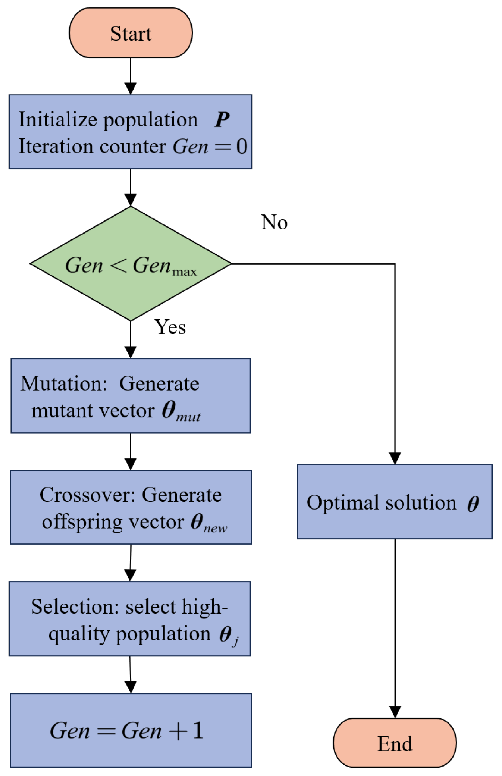
4.1.3. Configuration Optimization Algorithm

Various methods are available for solving the configuration problem of CDRMs, with the Jacobian-based velocity solution being the most widely used. However, this method calculates joint angular velocities and requires integration to obtain joint angle solutions. The iterative integration process can lead to significant cumulative errors, ultimately reducing the accuracy of the configuration solution. In contrast, position-based configuration solutions provide higher accuracy.
DE [32] is a typical evolutionary computation method that has been widely used in various optimization problems due to its efficiency and simplicity [33,34]. Numerous variants of DE have been proposed and successfully applied in various domains, including product design [35], image processing [36], energy systems [37], process planning [38], and other fields [39]. Among them, the fuzzy self-tuning DE [35] is a representative enhancement that incorporates a fuzzy logic mechanism to automatically calculate adaptive control parameters for each individual. This allows the algorithm parameters to be dynamically adjusted, improving overall optimization performance. Another enhanced DE incorporates chaotic opposition-based learning to enhance initialization and employs a dynamic selection mechanism based on Euclidean distance to improve the selection, thereby enhancing the robustness and search capability of the algorithm [38].
Compared to genetic algorithms (GAs), DE operates directly on real-valued variables, eliminating the need for complex binary encoding and decoding, which results in faster convergence. Furthermore, DE is relatively simple to implement and requires fewer control parameters, making it more accessible and computationally efficient than GA [40]. While particle swarm optimization (PSO) is also easy to implement, its performance heavily depends on parameter tuning, which requires considerable effort. Moreover, due to the lack of a mutation mechanism, PSO exhibits weaker global search capability. The performance of DE and its variants significantly surpasses that of PSO and its variants over a wide variety of problems, as has been indicated by studies [41,42]. Therefore, this paper employs the DE algorithm to solve the configuration optimization problem of the CDRM. The algorithm’s convergence behavior is defined by a termination criterion based on the maximum number of iterations. The flowchart of the configuration optimization based on improved DE algorithm is shown in Figure 1. The specific steps are detailed in Algorithm 1.
The mutation mechanism is a key factor influencing the effectiveness and stability of DE [43]. There are two primary mutation strategies: DE/rand/1/bin and DE/best/1/bin. The DE/rand/1/bin strategy provides broad search capability but has a relatively slow convergence speed. In contrast, the DE/best/1/bin strategy selects the individual with the highest fitness in the current population as the base vector, offering strong local exploitation ability and fast convergence. However, it is prone to premature convergence. To balance the global exploration and local exploitation capabilities of the DE algorithm, this study employs an adaptive mutation operator. The mutation operation is calculated as follows:
θ m u t = θ r 1 + F · θ r 2 θ r 3 , θ m u t = θ b + F · θ r 1 θ r 2 + θ r 3 θ r 4 , r a n d < 1 G e n / G e n max o t h e r w i s e
where θ m u t is the mutation vector, θ r 1 , θ r 2 , and θ r 3 are three different individuals randomly selected from the population, F is the scaling factor that controls the scaling of the differential vector, and θ b is the best individual in the population of the current generation.
The crossover operation is represented as follows:
θ n e w i = θ m u t i θ i r a n d i < C R o t h e r w i s e
where θ n e w i is the i-th element of the crossover vector, r a n d i represents a random number in the range of 0 to 1, and C R represents the crossover constant.
Algorithm 1 Configuration optimization based on improved DE algorithm
1:
Input:
2:
    Objective function: G θ ;
3:
    Population size: N;
4:
    Maximum iterations: G e n max ;
5:
    Mutation factor: F;
6:
    Crossover rate: C R .
7:
Initialize:
8:
    Initialize the population P = θ 1 , θ 2 , , θ N ;
9:
    Iteration counter G e n = 0 .
10:
Repeat:
11:
    While G e n < G e n max
12:
      For i = 1 to N
13:
         Mutation: Generate the mutated population vectors θ m u t according to (12).  
14:
         Crossover: Generate the new population θ n e w according to (13).  
15:
         Selection: Evaluate the fitness of G f i t θ n e w according (14).  
16:
         Update: Update solutions using (16).  
17:
      end
18:
    G e n G e n + 1 .
19:
    end
20:
Output:
21:
    Optimal solution: θ .
The fitness function considering the constraints is calculated as follows:
G f i t θ = G θ + G c θ
where G c θ is the constraint function:
G c θ = P θ P d e s 2
Update the solution by comparing the fitness function values of the new population with those of the previous population:
θ j = θ n e w θ j G f i t θ n e w G f i t θ j o t h e r w i s e .

4.2. Cable Tension Optimization

4.2.1. Tension Optimization Model

For a CDRM with n DOFs and m cables, its kinetostatic equilibrium equations can be expressed as follows:
AT = W
where A n × m represents the structure matrix, T m × 1 represents the cable tension vector, and W n × 1 represents the external wrench.
Due to redundant cable drives, multiple sets of cable tension solutions may exist for a given configuration. Under a specific configuration of the CDRM, the cable tension can be calculated as follows [19]:
T = A W + P n u l l λ
where A is the pseudoinverse of the structure matrix A . When A is of full row rank, A = A T AA T 1 . λ is an arbitrary column vector, and P n u l l represents the null space projection matrix of A , which can be calculated as follows:
P n u l l = E A A
where E represents the identity matrix.
To identify the optimal feasible solution that satisfies specific conditions, this problem can be formulated as the following minimization optimization problem:
min F T s . t . AT = W , T T l , T u
where T l and T u represent the lower and upper limits of T , respectively.

4.2.2. Optimization Objective Function

To prevent the cable tension from approaching its limits, the cable tension optimization objective function is formulated as a minimization problem and can be expressed as follows:
F s T = j = 1 m F s T j
where F s T j = T u j T l j 2 T u j T j T j T l j , T l j and T u j represent the j-th elements of T l and T u , respectively.
To obtain adjustable cable tension solutions for regulating the stiffness of the CDRM, a tension-level factor is introduced into the optimization objective function, which is formulated as a minimization problem and expressed as follows:
F T = j = 1 m F s T j F R T j
where F R T j is the tension regulation term, which can be calculated as follows:
F R T j = T j T R j 2
where T R j = τ R j · T u j T l j + T l j and τ R j is the j-th element of the tension-level factor τ R 0 , 1 .

4.2.3. Tension Optimization Algorithm

Due to its efficient computational capability and strong robustness, the gradient projection method (GPM) is widely applied to optimization problems in redundant systems [44,45]. This paper adopts a modified GPM to solve the cable tension solution. The convergence behavior of the algorithm is defined by two termination conditions: reaching the maximum number of iterations or when the projection vector becomes zero. The flowchart of the cable tension optimization based on the modified GPM is shown in Figure 2, and the specific steps are detailed in Algorithm 2.
Using the GPM to optimize T , (18) can be re-expressed as follows:
T = A W + k P n u l l F T
where k is a negative scalar, and F T represents the gradient of F T , which can be calculated as follows:
F T = F T T 1 F T T 2 F T T m T
Since the GPM searches for the optimal solution only within the null space, the cable tension solution must be expressed in the null space as follows:
T = k P n u l l F T
where T = T A W , representing a point in the null space of matrix A .
According to (26), the cable tension optimization problem in (20) can be re-expressed as follows:
min F T s . t . AT = 0 , T T l , T u
where T l = T l A W and T u = T u A W represent the upper and lower limits of T , respectively.
Algorithm 2 Cable tension optimization based on modified GPM
1:
Input:
2:
Structure matrix: A .
3:
External wrench: W .
4:
Maximum iterations: m a x _ i t e r .
5:
Initialize:
6:
Compute the cable tension solution T i n i t in the null space according to (26).
7:
Iteration counter k = 0 .
8:
Reapet:
9:
while  k < m a x _ i t e r  do
10:
    Set the current point T = T i n i t .
11:
    Calculate the gradient F T according to (30).
12:
    Calculate the projected vector v p according to (29).
13:
    if v p = 0 then
14:
        break
15:
    end if
16:
    Calculate the local minimum solution T l o c along v p according to (28).
17:
    Set T i n i t = T l o c .
18:
    Increment the iteration counter: k = k + 1 .
19:
end while
20:
Output:
21:
Optimal solution: T .
22:
Optimal cable tension solution: T = T + A W .
The search iteration process of the GPM is as follows:
T l o c = T i n i t D v ^ p
where T l o c represents the local minimum solution along the direction of the unit projection vector v ^ p , T i n i t represents the initial point of v ^ p , and D represents the distance between T i n i t and T l o c . The projection vector v p represents the steepest descent direction and can be calculated as follows:
v p = P n u l l F T i n i t
The gradient F T of F T can be calculated as follows:
F T T j = 1 2 G 1 G 2 + G 3 F T
where
  • G 1 = T u j T l j 2 T u j T j 2 T j T l j 2 ,
  • G 2 = 2 T u j T j T j T l j T j T R j ,
  • G 3 = 2 T j T l j T u j T j T R j 2 .

5. Case Study Example

To concisely illustrate the method proposed in this paper, this section uses a planar CDRM as a case example. It is worth noting that although the proposed method is illustrated using a planar CDRM, its underlying principles and optimization framework are general. When extended to three-dimensional or more complex CDRMs, the primary adjustment involves modifying the kinematic and kinetostatic models to account for the specific geometric structure. Since the structure of the optimization problem and the stiffness evaluation approach remain consistent, the proposed method retains its applicability across different spatial CDRMs. This adaptability makes it suitable for a wide range of CDRMs beyond the planar example presented in this study.

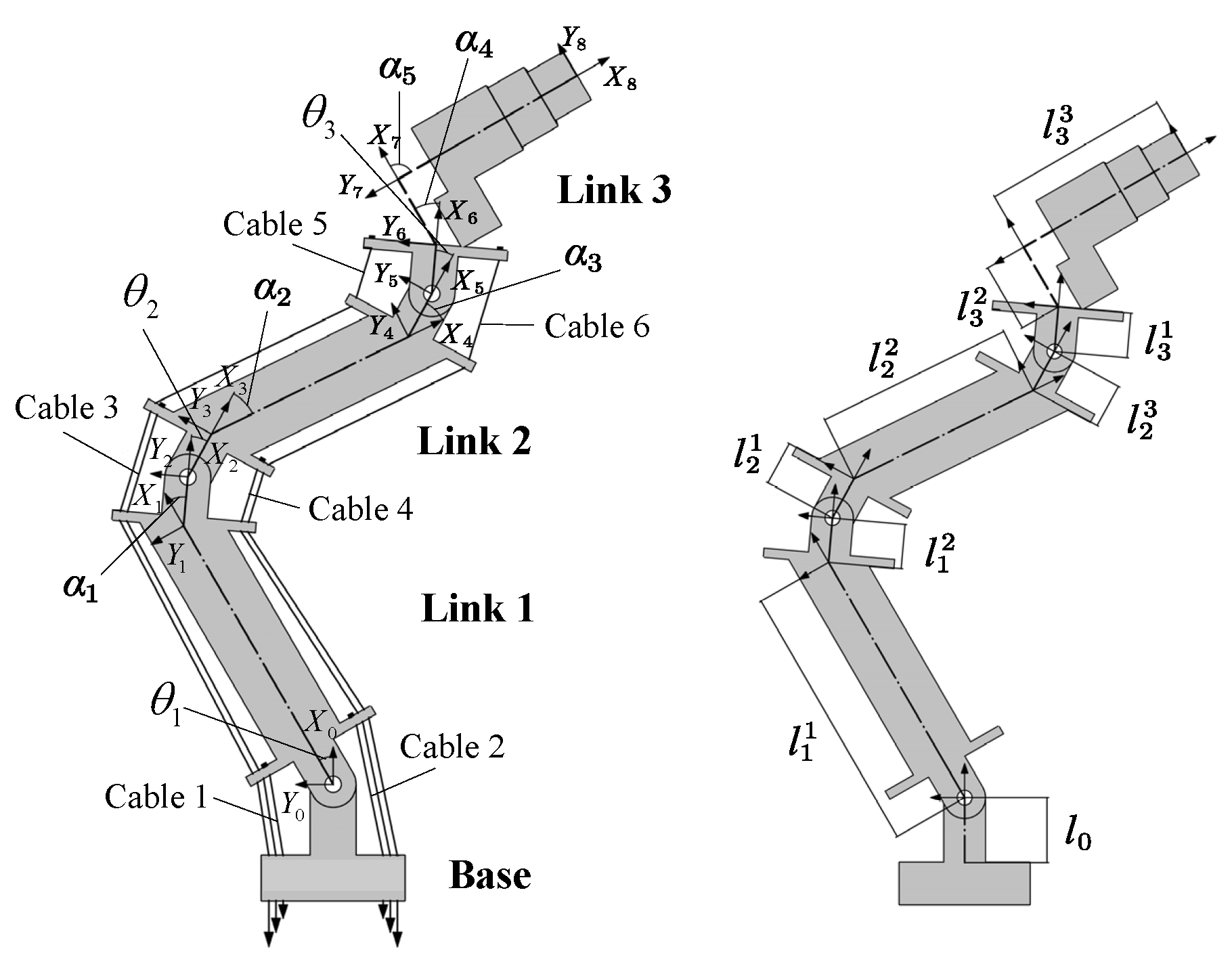
5.1. Structure of the Planar CDRM

As shown in Figure 3, the planar CDRM consists of three links connected by three rotary joints and is driven by six cables. The inertial frame is represented by frame 0, while the local frame of each link j is represented by frame j. The main parameters of the CDRM are listed in Table 1.

5.2. Kinematic Model

We use the D-H method to derive the forward kinematics model of the CDRM. In this example, the homogeneous transformation matrix from coordinate frame j to coordinate frame j 1 is expressed as follows:
T j j 1 = R j j 1 P j 0 1
where R j j 1 represents the rotation matrix from frame j to frame j 1 , and P j represents the translation vector.
According to (A2), the homogeneous transformation matrix from frame 6 to frame 0 is as follows:
T 6 0 = T 1 0 T 2 1 T 6 5
The end position vector of the CDRM in frame 0 is calculated as follows:
x y = C 1 + C 2 + C 3 S 1 + S 2 + S 3
where
  • C 1 = l 1 1 c θ 1 + l 1 2 c θ 1 α 1
  • C 2 = l 2 1 c θ 12 α 1 + l 2 2 c θ 12 α 12 + l 2 3 c θ 12 α 123
  • C 3 = l 3 1 c θ 123 α 123 + l 3 2 c θ 123 α 1234 + l 3 3 c θ 123 α 12345
  • S 1 = l 1 1 s θ 1 + l 1 2 s θ 1 α 1
  • S 2 = l 2 1 s θ 12 α 1 + l 2 2 s θ 12 α 12 + l 2 3 s θ 12 α 123
  • S 3 = l 3 1 s θ 123 α 123 + l 3 2 s θ 123 α 1234 + l 3 3 s θ 123 α 12345
  • θ 12 n = θ 1 + θ 2 + + θ n , α 12 n = α 1 + α 2 + + α n
  • α 12 n θ 12 n = θ 12 n + α 12 n , s θ = sin θ , c θ = cos θ .

5.3. Kinetostatic Model

Reciprocal screw theory establishes a mathematical framework between wrenches and twists, offering an effective tool for analyzing the complex relationships between forces and motions [46]. Based on this theory, this paper develops the kinetostatic model of the CDRM. The screw representation of the CDRM is illustrated in Figure 4, with the specific steps outlined in Algorithm 3. The detailed calculation process can be found in [47]. The detailed derivation of the CDRM’s kinetostatic model is provided in Appendix A.
The static equilibrium equation of the CDRM can be expressed as follows:
AT = W
where
  • A = a 11 ε 11 a 12 ε 12 a 13 ε 13 a 14 ε 14 a 15 ε 15 a 16 ε 16 0 0 a 23 ε 23 a 24 ε 24 a 25 ε 25 a 26 ε 26 0 0 0 0 a 35 ε 35 a 36 ε 36
  • T = T 1 T 2 T 3 T 4 T 5 T 6 T
  • W = λ 1 1 + λ 2 1 + λ 3 1 $ ^ 1 λ 2 2 + λ 3 2 $ ^ 2 λ 3 3 $ ^ 3 .
Algorithm 3 Kinetostatic model of CDRMs
Input: 
Structural parameters of the CDRM, configuration of the CDRM, external wrench applied to each link $ i e w .
Step 1: 
Calculate the unit screws of twists $ ^ i and reciprocal wrenches $ ^ i r ;
Step 2: 
Express external wrenches as linear combinations of reciprocal screws and calculate the passive joint torques generated by external wrenches;
Step 3: 
Express the cable tension as linear combinations of reciprocal screws and calculate the active joint torques provided by the cable tension;
Step 4: 
Determine the kinetostatic model by balancing the passive joint torques with the active joint torques;
Output: 
Kinetostatic equilibrium equation of the CDRM.

5.4. Stiffness Regulation

5.4.1. Configuration Optimization

In this example, the motion range of each joint is set to 35 , 35 . The configuration optimization problem can be formulated as follows:
min i = 1 3 θ u i θ l i 2 θ i θ R i 2 θ u i θ i θ i θ l i s . t . x y = x d e s y d e s , θ i 35 , 35

5.4.2. Cable Tension Optimization

The cable tension range is set to 1 , 500 N . The cable tension optimization problem can be expressed as follows:
min j = 1 6 T u j T l j 2 T j T R j 2 T u j T j T j T l j s . t . AT = 0 , T i 500 A W , 1 A W

6. Numerical Simulation

This section validates the method proposed in this paper through numerical simulations. The geometric parameters of the CDRM used in the simulation are shown in Table 1. All algorithms are implemented using Python 3.8.

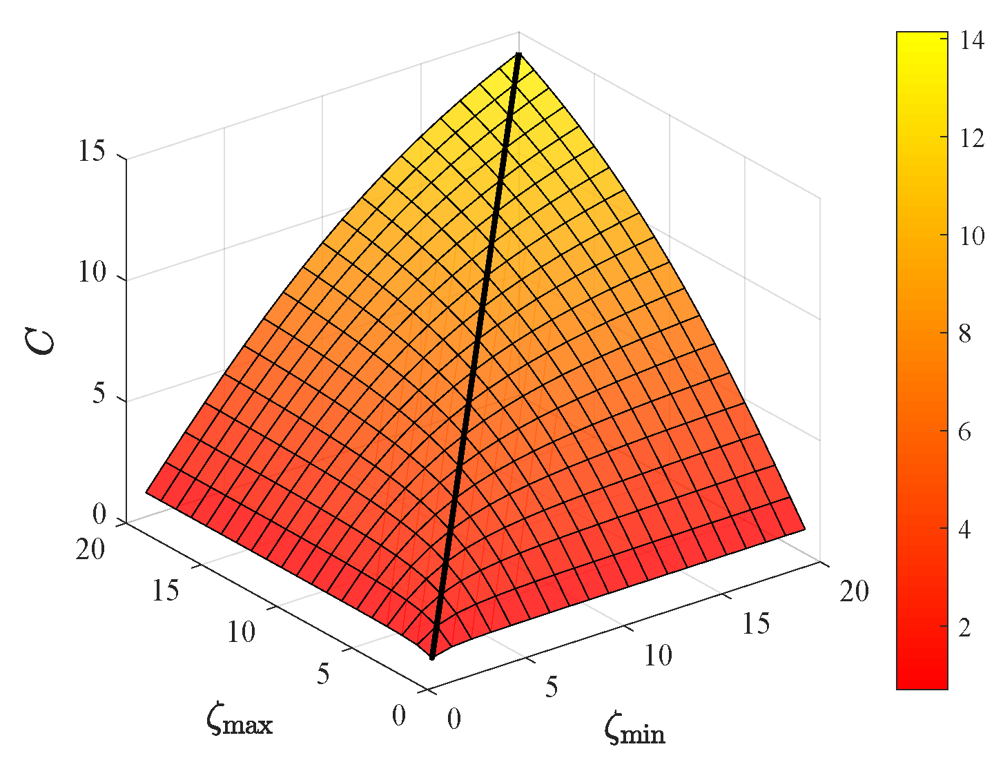
6.1. Stiffness Evaluation Metrics

Metrics for evaluating the magnitude of stiffness include the trace of the stiffness matrix [48], eigenvalues [30], and the determinant [49]. Among these, the determinant of the stiffness matrix is commonly used as a metric for evaluating the stiffness magnitude:
M = det K = ζ 1 ζ 2 ζ n
where ζ i i = 1 , 2 , , n represents the eigenvalues of the stiffness matrix K .
However, the determinant reflects only the magnitude of stiffness and does not account for directional information. The condition number (CN) offers a quantitative metric of the uniformity of the stiffness distribution [16], and its definition is as follows:
CN = ζ max ζ min
where ζ min and ζ max represent the minimum and maximum eigenvalues of the stiffness matrix, respectively.
To comprehensively evaluate both the magnitude and direction of stiffness, this paper introduces a new metric for assessing the stiffness matrix:
C = ζ min 2 × ζ max 2 ζ min 2 + ζ max 2
Figure 5 illustrates the relationship between the stiffness evaluation metric C, ζ min , and ζ max . It can be observed that when ζ min = ζ max , a spine is formed (as indicated by the black line). Furthermore, as ζ min and ζ max increase, the height of the spine also rises. Therefore, a larger C value indicates better performance of the stiffness matrix in terms of both stiffness magnitude and isotropy.

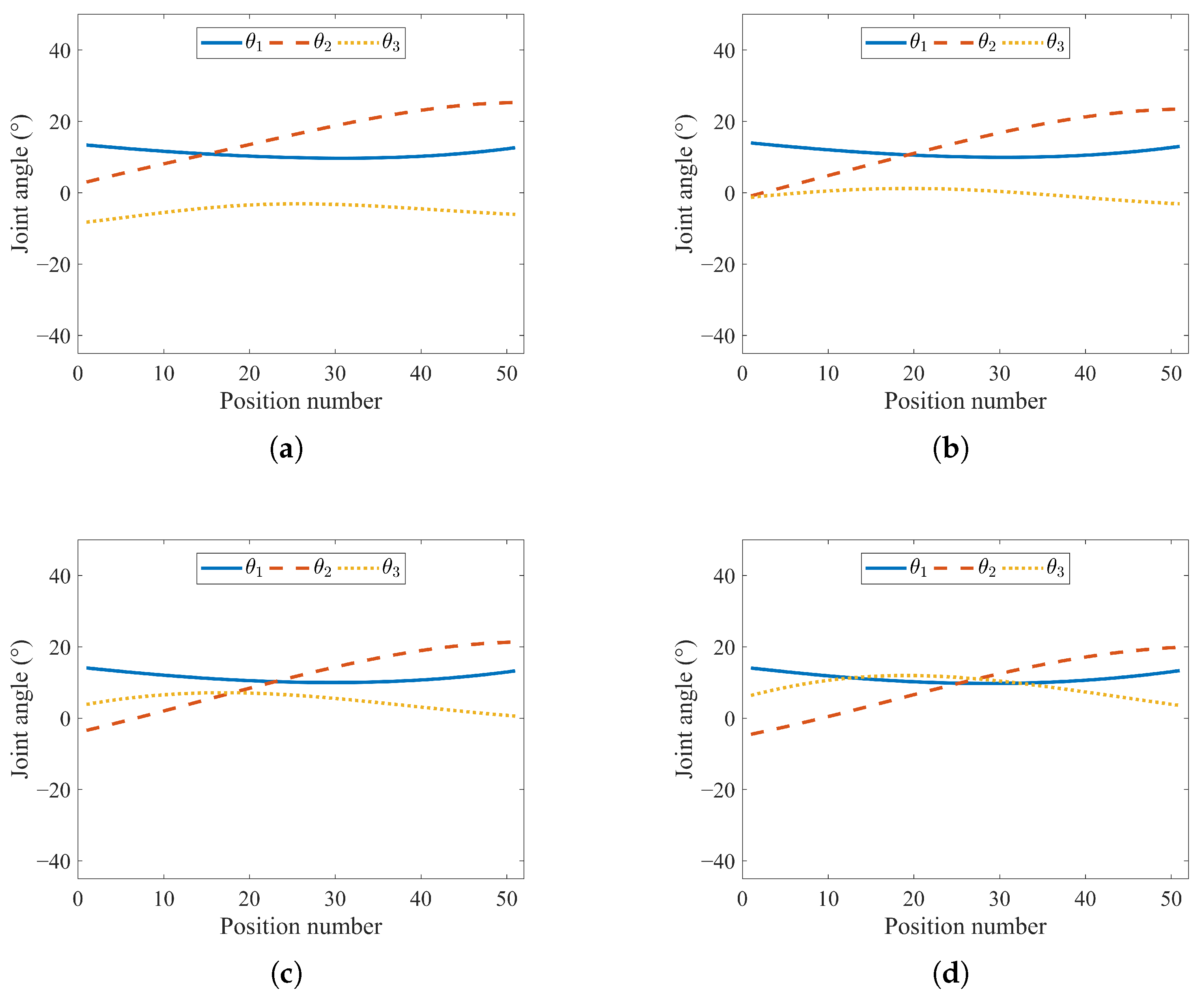
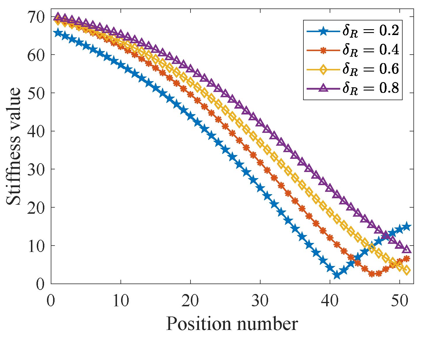
6.2. Configuration Optimization

We set the rotation angles of the first two joints to 10° and 15°, respectively, while varying the rotation angle of the third joint from −25° to 25° in increments of 5° for each step. The resulting motion path of the end-effector is shown in Figure 6. The improved DE algorithm is used to determine the configuration solutions of the manipulator for each pose. In the configuration optimization problem, the decision variables are the joint angles of the manipulator, with a dimensionality of D = 3 . Following the parameter settings recommended in [32], the population size used in the DE algorithm is set to N p = 30 , the mutation scale factor is set to F = 0.5 , and the crossover probability is set to C R = 0.9 [37].
Figure 7 displays the configuration solutions along this path for four different motion-level factors δ R ( δ R i i = 1 , 2 , 3 ) of 0.2 , 0.4 , 0.6 and 0.8 . It can be observed that when δ R = 0.2 , the configuration solutions are close to the lower limit of the joint motion range, whereas when δ R = 0.8 , they approach the upper limit of the joint motion range. For δ R = 0.4 and δ R = 0.6 , the configuration solutions are further from both limits. These results indicate that adjusting the motion-level factor δ R allows for agile modification of the configuration solutions.
To investigate the impact of configuration on the stiffness of the CDRM, we calculate the stiffness values of the configurations under various motion-level factors at the same desired position. To ensure consistency, the cable tension-level factor τ R ( τ R j j = 1 , 2 , , 6 ) is set to 0.1 . Figure 8 presents the stiffness results for the configuration solutions corresponding to different motion-level factors. Notably, the stiffness varies with changes in the motion-level factors at the same desired position. When δ R = 0.8 , the stiffness performance of the CDRM is optimal in most positions. When δ R = 0.2 , its stiffness performance is weaker in most positions but stronger in a few. These results demonstrate that modifying the motion-level factor δ R can effectively regulate the stiffness of the CDRM.

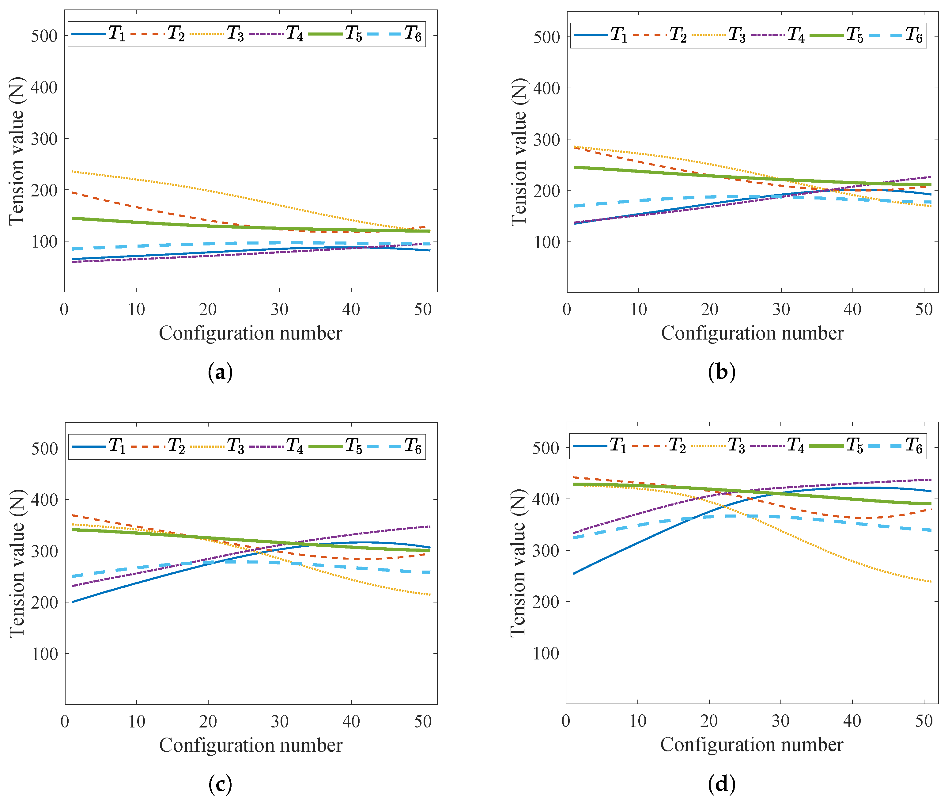
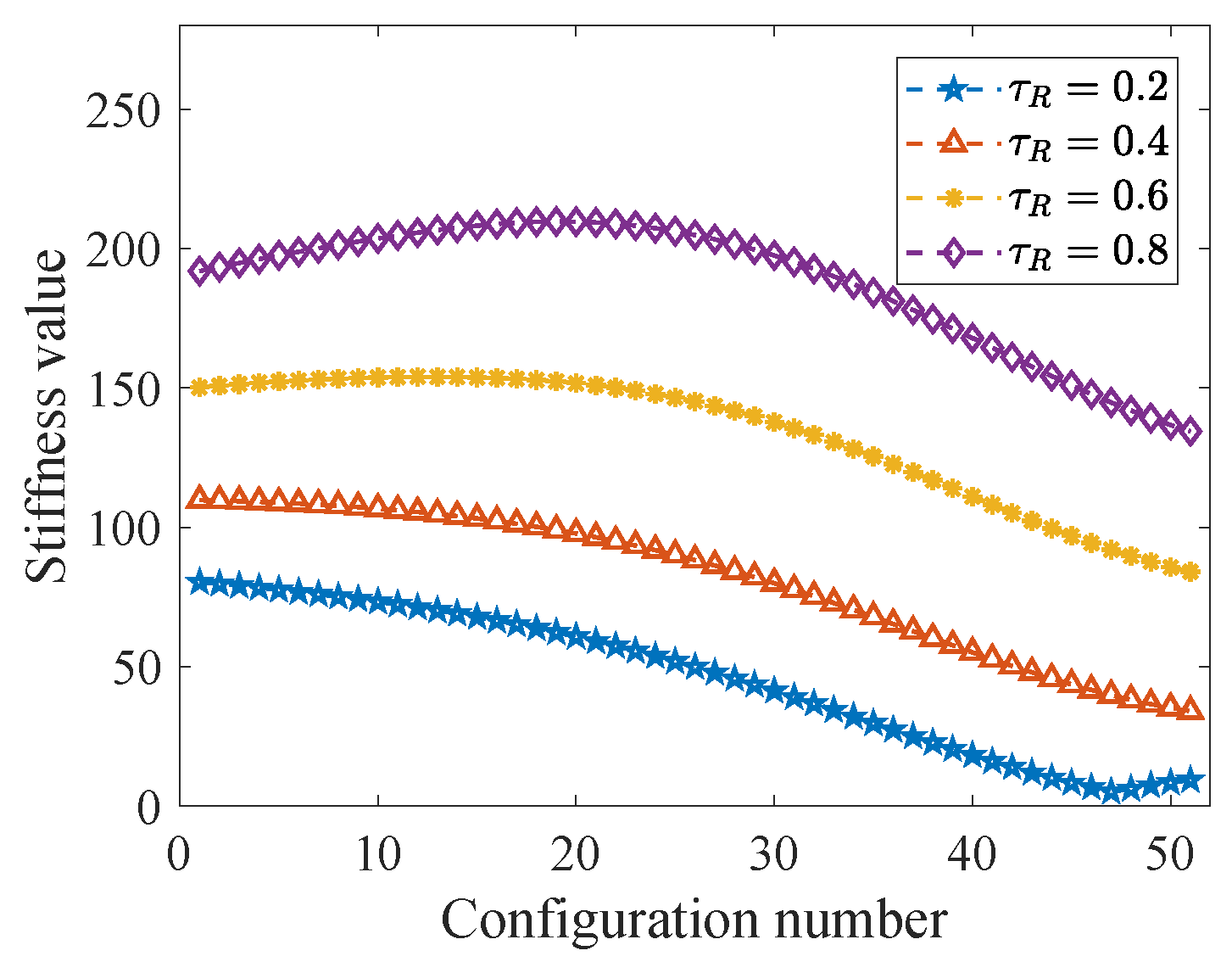
6.3. Cable Tension Optimization

To investigate the influence of cable tension on the stiffness of the CDRM, the configuration solutions along the path are calculated with a uniform motion-level factor of δ R = 0.1 . The improved gradient projection method is used to solve the cable tension solutions for each configuration. The algorithm’s maximum number of iterations is set to 10. Figure 9 presents the tension solutions obtained under these configurations for four different tension-level factors τ R of 0.2 , 0.4 , 0.6 and 0.8 . It can be observed that when τ R = 0.2 , the tension solutions are close to the lower limit of the tension range, while when τ R = 0.8 , the tension solutions approach the upper limit. For τ R = 0.4 and τ R = 0.6 , the tension solutions fall in the middle of the range. These results suggest that adjusting the tension-level factor effectively regulates the tension solutions.
Figure 10 presents the stiffness results for the tension solutions corresponding to different tension-level factors. It is clear that there are differences in stiffness across different tension-level factors. Notably, as the tension-level factor increases, the stiffness of the CDRM rises accordingly, demonstrating that adjusting the tension-level factor can effectively regulate the stiffness of the CDRM.

6.4. Combined Optimization of Configuration and Cable Tension

We set τ R = 0.1 at the end position of the path and calculated the stiffness values for δ R ranging from 0.1 to 0.9 in increments of 0.1 . The stiffness regulation results achieved by individually optimizing the configuration, with a minimum stiffness of 0.25 and a maximum stiffness of 15.68 .
At the same position, with the motion-level factor δ R = 0.1 , the stiffness values for τ R ranging from 0.1 to 0.9 in increments of 0.1 are calculated. The stiffness regulation results achieved by individually optimizing the cable tension, with a minimum stiffness of 4.34 and a maximum stiffness of 159.29 .
Figure 11 illustrates the stiffness regulation results achieved through combined optimization of the configuration and cable tension. It can be observed that when δ R = 0.5 and τ R = 0.1 , the stiffness of the CDRM is minimized at 0.25 . In contrast, when δ R = 0.9 and τ R = 0.9 , the stiffness reaches its maximum at 211.8 . These results indicate that combined optimization provides a broader range of stiffness regulation compared to individual optimization of configuration or cable tension.
To compare the effectiveness of stiffness regulation achieved through configuration optimization, cable tension optimization, and their combined optimization, Table 2 presents the stiffness regulation ranges of these three methods at different positions along the path. As shown in the table, all three methods can regulate stiffness within a certain range at the same positions. In this case study, the stiffness regulation range achieved through configuration optimization is generally narrower than that of cable tension optimization. Notably, the stiffness regulation range obtained by the combined optimization of configuration and cable tension encompasses the ranges achieved by the other two methods.
The range span ratio (RSR) is a metric used to evaluate the improvement in the stiffness regulation range, and it is defined as follows:
R S R = R S 1 R S 2
where R S 1 = R S 1 max R S 1 min represents the range span of S 1 , and R S 2 = R S 2 max R S 2 min represents the range span of S 2 .
Compared to configuration optimization alone, the combined optimization method achieves a maximum RSR of 17.78 and an average RSR of 12.60, indicating a substantial enhancement in stiffness regulation capacity. When compared with cable tension optimization alone, the combined method still shows improvements, with a maximum RSR of 1.37 and an average RSR of 1.10. These results indicate that the proposed combined optimization method offers a broader range of stiffness regulation.
To assess the computational efficiency of the proposed optimization method, we conduct 50 independent runs for a single target pose on a computer (Intel Core i7-11800H (Intel Corporation, Santa Clara, CA, USA), 2.3 GHz, 16 GB RAM). The average computation time per run is 0.16 s. The results demonstrate that the method is suitable for offline planning, allowing the pre-computation and storage of stiffness parameters obtained through combined optimization of the manipulator configuration and cable tension, which can be easily accessed in real time during actual operation.

7. Conclusions

This work presents a novel method for regulating the stiffness of CDRMs through the combined optimization of configuration and cable tension. A stiffness model is established to systematically analyze the effects of both configuration and cable tension on the manipulator’s stiffness. By leveraging the redundancy in both DOFs and actuation cables, the proposed method performs combined optimization to effectively regulate stiffness. Specifically, a configuration optimization objective function is formulated by introducing motion-level factors, and an improved DE algorithm is employed to obtain adjustable configuration solutions for each pose. This allows for stiffness regulation by manipulating the motion-level factors. Similarly, a tension optimization objective function is constructed with tension-level factors, and a modified GPM is used to compute adjustable cable tension solutions, enabling further stiffness regulation through manipulation of the tension-level factors. This study verifies the feasibility and effectiveness of the proposed method through simulations on a planar CDRM. The results demonstrate that effective stiffness regulation of the manipulator can be achieved by adjusting the motion-level and tension-level factors. The combined optimization method achieves a maximum RSR of 17.78 and an average RSR of 12.60 compared to configuration optimization, and a maximum RSR of 1.37 and an average RSR of 1.10 compared to tension optimization. These results demonstrate that the proposed combined method provides a broader stiffness regulation range.
Although the proposed method effectively achieves stiffness regulation under quasi-static conditions, it does not fully account for dynamic factors such as inertia and vibration that arise during dynamic tasks. As part of future work, we plan to incorporate dynamic modeling to address these factors and enable stiffness regulation under dynamic conditions. Furthermore, we intend to develop a physical prototype to experimentally validate the effectiveness of the proposed method under realistic operating conditions.

Author Contributions

Conceptualization, Z.L. and P.Q.; methodology, Z.L.; software, Z.L.; investigation, Z.L. and P.Q.; writing—original draft preparation, Z.L.; writing—review and editing, S.D. All authors have read and agreed to the published version of the manuscript.

Funding

This research received no external funding.

Institutional Review Board Statement

Not applicable.

Informed Consent Statement

Not applicable.

Data Availability Statement

The original contributions presented in this study are included in the article. Further inquiries can be directed to the corresponding author.

Conflicts of Interest

The authors declare no conflicts of interest.

Abbreviations

The following abbreviations are used in this manuscript:
CDRMCable-Driven Redundant Manipulator
DOFDegree of Freedom
DEDifferential Evolution
GAGenetic Algorithms
PSOParticle Swarm Optimization
GPMGradient Projection Method
RSRRange Span Ratio

Appendix A. Kinetostatic Model

(1)
Determine the Unit Screws of Twists and Reciprocal Wrenches
The unit screw of the twist of each joint of the CDRM relative to the inertial frame can be expressed as follows:
$ ^ 1 = 0 0 1 0 0 0 T
$ ^ 2 = 0 0 1 l 1 1 s θ 1 + l 1 2 s α 1 θ 1 l 1 1 c θ 1 l 1 2 c α 1 θ 1 0 T
$ ^ 3 = 0 0 1 S 3 C 3 0 T
where
  • S 3 = l 1 1 s θ 1 + l 1 2 s α 1 θ 1 + l 2 1 s α 1 θ 12 + l 2 2 s α 12 θ 12 + l 2 3 s α 123 θ 12
  • C 3 = l 1 1 c θ 1 l 1 2 c α 1 θ 1 l 2 1 c α 1 θ 12 l 2 2 c α 12 θ 12 l 2 3 c α 123 θ 12
  • θ 12 n = θ 1 + θ 2 + + θ n , α 12 n = α 1 + α 2 + + α n
  • α 12 n θ 12 n = α 12 n + θ 12 n , s θ = sin θ , c θ = cos θ .
Through the analysis of the geometric relationships of the CDRM, the unit screws of the reciprocal wrench corresponding to the twist of each joint can be expressed as follows:
$ ^ 1 r = c α 1 θ 1 + γ 2 s α 1 θ 1 + γ 2 0 0 0 l 1 s γ 1 γ 2 T
$ ^ 2 r = c ϕ s ϕ 0 0 0 0 T
$ ^ 3 r = c φ s φ 0 0 0 0 T
where
  • l 1 = l 1 1 2 + l 1 2 2 l 1 1 l 1 2 cos π + α 1
  • γ 1 = atan 2 l 1 1 s α 1 , l 1 2 + l 1 1 c α 1 , γ 2 = atan 2 γ 2 y , γ 2 x
  • γ 2 y = l 2 1 s θ 2 + l 2 2 s α 2 θ 2 + l 2 3 s α 23 θ 2
  • γ 2 x = l 2 1 c θ 2 + l 2 2 c α 2 θ 2 + l 2 3 c α 23 θ 2
  • ϕ = atan 2 ϕ y , ϕ x , φ = atan 2 φ y , φ x
  • ϕ y = l 1 1 s θ 1 + l 1 2 s α 1 θ 1 + l 2 1 s α 1 θ 12 + l 2 2 s α 12 θ 12 + l 2 3 s α 123 θ 12
  • ϕ x = l 1 1 c θ 1 + l 1 2 c α 1 θ 1 + l 2 1 c α 1 θ 12 + l 2 2 c α 12 θ 12 + l 2 3 c α 123 θ 12
  • φ y = l 1 1 s θ 1 + l 1 2 s α 1 θ 1 , φ x = l 1 1 c θ 1 + l 1 2 c α 1 θ 1 .
(2)
Calculate the passive joint torques
The external wrenches $ j e w acting on the j-th link of the CDRM can be expressed using reciprocal screws as follows:
$ j e w = 1 λ j $ ^ 1 r + 2 λ j $ ^ 2 r + 3 λ j $ ^ 3 r , j = 1 , 2 , 3
The passive torque Γ j p at each joint j-th generated by the external wrench can be calculated as follows:
Γ j p = k = j 3 λ k j $ ^ j r $ ^ j , j = 1 , 2 , 3
(3)
Calculate the active joint torques
The unit screw of the tension in the subsegment of the i-th cable acting on the j-th to k-th link can be expressed using reciprocal screws as follows:
$ ^ i 1 1 k 1 = 1 ν i 1 1 k 1 $ ^ 1 r + 2 ν i 1 1 k 1 $ ^ 2 r + 3 ν i 1 1 k 1 $ ^ 3 r
$ ^ i 2 2 k 2 = 1 ν i 2 2 k 2 $ ^ 1 r + 2 ν i 2 2 k 2 $ ^ 2 r + 3 ν i 2 2 k 2 $ ^ 3 r
$ ^ i 3 3 k 3 = 1 ν i 3 3 k 3 $ ^ 1 r + 2 ν i 3 3 k 3 $ ^ 2 r + 3 ν i 3 3 k 3 $ ^ 3 r
where i 1 = 1 , 2 , , 6 , k 1 = 0 , 2 , i 2 = 3 , 4 , 5 , 6 , k 2 = 1 , 3 , and i 3 = 5 , 6 , k 3 = 2 .
Considering the coupling between the cables, the active torque at the k-th joint can be calculated by superimposing the tensions of all cable subsegments between the k-th link and the end link as follows:
Γ 1 a = a 11 T 1 1 0 + a 12 T 2 1 0 + + a 16 T 6 1 0 $ ^ 1
Γ 2 a = a 23 T 3 2 1 + a 24 T 4 2 1 + + a 26 T 6 2 1 $ ^ 2
Γ 3 a = a 35 T 5 3 2 + a 36 T 6 3 2 $ ^ 3
where
  • a 1 i = 1 ν i 1 0 , i = 1 , 2 , , 6 , a 2 i = 2 ν i 2 1 , i = 3 , 4 , 5 , 6
  • a 3 i = 3 ν i 3 2 , i = 5 , 6 , $ ^ n = $ ^ n r $ ^ n , n = 1 , 2 , 3 .
Considering the effect of friction on the tension of different cable subsegments. The active torque at each joint can be calculated as follows:
Γ 1 a = a 11 ε 11 T 1 + a 12 ε 12 T 2 + + a 16 ε 16 T 6 $ ^ 1
Γ 2 a = a 23 ε 23 T 3 + a 24 ε 24 T 4 + + a 26 ε 26 T 6 $ ^ 2
Γ 3 a = a 35 ε 35 T 5 + a 36 ε 36 T 6 $ ^ 3
where
  • ε 1 i = e D i r v i 0 μ β i 0 , i = 1 , 2 , , 6
  • ε 2 i = e j = 0 1 D i r v i j μ β i j , i = 3 , 4 , 5 , 6
  • ε 3 i = e j = 0 2 D i r v i j μ β i j , i = 5 , 6 .
(4)
Determine the Static Equilibrium Equation
When the active and passive torques at each joint of the manipulator counteract each other, the manipulator remains in static equilibrium. The static equilibrium equation of the CDRM can be expressed as follows:
AT = W
where
  • A = a 11 ε 11 a 12 ε 12 a 13 ε 13 a 14 ε 14 a 15 ε 15 a 16 ε 16 0 0 a 23 ε 23 a 24 ε 24 a 25 ε 25 a 26 ε 26 0 0 0 0 a 35 ε 35 a 36 ε 36
  • T = T 1 T 2 T 3 T 4 T 5 T 6 T
  • W = λ 1 1 + λ 2 1 + λ 3 1 $ ^ 1 λ 2 2 + λ 3 2 $ ^ 2 λ 3 3 $ ^ 3 .

References

  1. Li, W.S.; Huang, X.; Yan, L.; Cheng, H.Y.; Liang, B.; Xu, W.F. Force Sensing and Compliance Control for a Cable-Driven Redundant Manipulator. IEEE-ASME Trans. Mechatron. 2024, 29, 777–788. [Google Scholar] [CrossRef]
  2. Xu, W.F.; Liu, T.L.; Li, Y.M. Kinematics, Dynamics, and Control of a Cable-Driven Hyper-Redundant Manipulator. IEEE-ASME Trans. Mechatron. 2018, 23, 1693–1704. [Google Scholar] [CrossRef]
  3. Omisore, O.M.; Han, S.P.; Xiong, J.; Yang, J.; Li, Z.; Wang, L. A Review on Flexible Robotic Systems for Minimally Invasive Surgery. IEEE Trans. Syst. Man Cybern.-Syst. 2022, 52, 631–644. [Google Scholar] [CrossRef]
  4. Hong, W.Z.; Xie, L.; Liu, J.H.; Sun, Y.J.; Li, K.Y.; Wang, H.S. Development of a Novel Continuum Robotic System for Maxillary Sinus Surgery. IEEE-ASME Trans. Mechatron. 2018, 23, 1226–1237. [Google Scholar] [CrossRef]
  5. Seyfi, N.S.; Khalaji, A.K. Robust control of a cable-driven rehabilitation robot for lower and upper limbs. ISA Trans. 2022, 125, 268–289. [Google Scholar] [CrossRef] [PubMed]
  6. Mao, Y.; Agrawal, S.K. Design of a cable-driven arm exoskeleton (carex) for neural rehabilitation. IEEE Trans. Robot. 2012, 28, 922–931. [Google Scholar] [CrossRef]
  7. Lou, Y.N.; Di, S.C. Design of a cable-driven auto-charging robot for electric vehicles. IEEE Access 2020, 8, 15640–15655. [Google Scholar] [CrossRef]
  8. Wang, M.F.; Dong, X.; Ba, W.M.; Mohammad, A.; Axinte, D.; Norton, A. Design, modelling and validation of a novel extra slender continuum robot for in-situ inspection and repair in aeroengine. Robot. Comput.-Integr. Manuf. 2021, 67, 102054. [Google Scholar] [CrossRef]
  9. Endo, G.; Horigome, A.; Palmer, D.; Takata, A. Super dragon: A 10-m-long-coupled tendon-driven articulated manipulator. IEEE Robot. Autom. Lett. 2019, 4, 934–941. [Google Scholar] [CrossRef]
  10. Pang, S.X.; Shang, W.W.; Dai, S.Q.; Deng, J.; Zhang, F.; Zhang, B.; Cong, S. Stiffness optimization of cable-driven humanoid manipulators. IEEE/ASME Trans. Mechatron. 2024, 29, 4168–4178. [Google Scholar] [CrossRef]
  11. Lang, G.D.; Gao, Y.S.; Luo, Z.W.; Liang, G.L.; Zhu, Y.H.; Zhao, J. Kinematic analysis for the spatial interlocking 3-uu mechanism with the wide range of motion. IEEE Robot. Autom. Lett. 2024, 9, 3926–3931. [Google Scholar] [CrossRef]
  12. Xu, H.J.; Meng, D.S.; Li, Y.N.; Wang, X.Q.; Liang, B. A novel cable-driven joint module for space manipulators: Design, modeling, and characterization. IEEE/ASME Trans. Mechatron. 2024, 29, 2044–2055. [Google Scholar] [CrossRef]
  13. Gao, Y.M.; Lv, G.K.; Zhao, S.; Ding, N.; Mu, Z.G. An analytical variable-stiffness method for the fine control of concentric cable-driven manipulators. IEEE Trans. Syst. Man Cybern. Syst. 2024, 54, 5434–5443. [Google Scholar] [CrossRef]
  14. Sanjeevi, N.S.S.; Vashista, V. Stiffness modulation of a cable-driven leg exoskeleton for effective human-robot interaction. Robotica 2021, 39, 2172–2192. [Google Scholar] [CrossRef]
  15. Ramadoss, V.; Sagar, K.; Ikbal, M.S.; Zlatanov, D.; Zoppi, M. Modeling and stiffness evaluation of tendon-driven robot for collaborative human-robot interaction. In Proceedings of the 2021 IEEE International Conference on Intelligence and Safety for Robotics (IEEE-ISR), Electr Network, Nagoya, Japan, 4–6 March 2021; pp. 233–238. [Google Scholar]
  16. Sanjeevi, N.S.S.; Vashista, V. Stiffness modulation of a cable-driven serial-chain manipulator via cable routing alteration. J. Mech. Robot. 2023, 15, 021009. [Google Scholar] [CrossRef]
  17. Yang, K.S.; Yang, G.L.; Chen, S.L.; Wang, Y.; Zhang, C.; Fang, Z.J.; Zheng, T.J.; Wang, C.C. Study on stiffness-oriented cable tension distribution for a symmetrical cable-driven mechanism. Symmetry 2019, 11, 1158. [Google Scholar] [CrossRef]
  18. Yang, K.S.; Yang, G.L.; Wang, Y.; Zhang, C.; Chen, S.L. Stiffness-oriented cable tension distribution algorithm for a 3-dof cable-driven variable-stiffness module. In Proceedings of the 2017 IEEE ASME International Conference on Advanced Intelligent Mechatronics (AIM), Munich, Germany, 3–7 July 2017; pp. 454–459. [Google Scholar]
  19. Lim, W.B.; Yeo, S.H.; Yang, G.L. Optimization of tension distribution for cable-driven manipulators using tension-level index. IEEE/ASME Trans. Mechatron. 2014, 19, 676–683. [Google Scholar] [CrossRef]
  20. Abdolshah, S.; Zanotto, D.; Rosati, G.; Agrawal, S.K. Optimizing stiffness and dexterity of planar adaptive cable-driven parallel robots. J. Mech. Robot. 2017, 9, 031004. [Google Scholar] [CrossRef]
  21. Orekhov, A.L.; Simaan, N. Directional stiffness modulation of parallel robots with kinematic redundancy and variable stiffness joints. J. Mech. Robot. 2019, 11, 051003. [Google Scholar] [CrossRef]
  22. Chen, S.T.; Zhou, G.Z.; Li, D.C.; Song, Z.A.; Chen, F.F. Soft robotic joints with anisotropic stiffness by multiobjective topology optimization. IEEE/ASME Trans. Mechatron. 2024, 29, 1064–1075. [Google Scholar] [CrossRef]
  23. Hong, W.Z.; Feng, F.; Xie, L.; Yang, G.Z. A two-segment continuum robot with piecewise stiffness for maxillary sinus surgery and its decoupling method. IEEE/ASME Trans. Mechatron. 2022, 27, 4440–4450. [Google Scholar] [CrossRef]
  24. Yeo, S.H.; Yang, G.; Lim, W.B. Design and analysis of cable-driven manipulators with variable stiffness. Mech. Mach. Theory 2013, 69, 230–244. [Google Scholar] [CrossRef]
  25. Liu, T.L.; Xu, W.F.; Yang, T.W.; Li, Y.M. A hybrid active and passive cable-driven segmented redundant manipulator: Design, kinematics, and planning. IEEE/ASME Trans. Mechatron. 2021, 26, 930–942. [Google Scholar] [CrossRef]
  26. Zhao, B.; Zeng, L.Y.; Wu, Z.H.; Xu, K. A continuum manipulator for continuously variable stiffness and its stiffness control formulation. Mech. Mach. Theory 2020, 149, 103746. [Google Scholar] [CrossRef]
  27. Ma, N.; Yu, J.J.; Dong, X.; Axinte, D. Design and stiffness analysis of a class of 2-dof tendon driven parallel kinematics mechanism. Mech. Mach. Theory 2018, 129, 202–217. [Google Scholar] [CrossRef]
  28. Pang, S.X.; Shang, W.W.; Zhang, F.; Zhang, B.; Cong, S. Design and stiffness analysis of a novel 7-dof cable-driven manipulator. IEEE Robot. Autom. Lett. 2022, 7, 2811–2818. [Google Scholar] [CrossRef]
  29. Huang, J.L.; Clement, R.; Sun, Z.H.; Wang, J.Z.; Zhang, W.J. Global stiffness and natural frequency analysis of distributed compliant mechanisms with embedded actuators with a general-purpose finite element system. Int. J. Adv. Manuf. Technol. 2013, 65, 1111–1124. [Google Scholar] [CrossRef]
  30. Alamdari, A.; Haghighi, R.; Krovi, V. Stiffness modulation in an elastic articulated-cable leg-orthosis emulator: Theory and experiment. IEEE Trans. Robot. 2018, 34, 1266–1279. [Google Scholar] [CrossRef]
  31. Zhang, L.Y.; Gao, Y.M.; Mu, Z.G.; Yan, L.; Li, Z.X.; Gao, M.W. A variable-stiffness planning method considering both the overall configuration and cable tension for hyper-redundant manipulators. IEEE-ASME Trans. Mechatron. 2024, 29, 659–667. [Google Scholar] [CrossRef]
  32. Storn, R.; Price, K. Differential evolution—A simple and efficient heuristic for global optimization over continuous spaces. J. Glob. Optim. 1997, 11, 341–359. [Google Scholar] [CrossRef]
  33. Liang, J.; Lin, H.Y.; Yue, C.T.; Yu, K.J.; Guo, Y.; Qiao, K.J. Multiobjective differential evolution with speciation for constrained multimodal multiobjective optimization. IEEE Trans. Evol. Comput. 2023, 27, 1115–1129. [Google Scholar] [CrossRef]
  34. Cai, Z.H.; Gao, S.C.; Yang, X.; Zhou, M.C. Multiselection-based differential evolution. IEEE Trans. Syst. Man Cybern.-Syst. 2024, 54, 7318–7330. [Google Scholar] [CrossRef]
  35. Tsafarakis, S.; Zervoudakis, K.; Andronikidis, A.; Altsitsiadis, E. Fuzzy self-tuning differential evolution for optimal product line design. Eur. J. Oper. Res. 2020, 287, 1161–1169. [Google Scholar] [CrossRef]
  36. Hielscher, T.; Hadigheh, S.A. Optimizing memory-efficient multimodal networks for image classification using differential evolution. Appl. Soft Comput. 2025, 171, 112714. [Google Scholar] [CrossRef]
  37. Dinh, Q.V.; Dinh, V.N.; Leahy, P.G. A differential evolution model for optimising the size and cost of electrolysers coupled with offshore wind farms. Int. J. Hydrogen Energy 2025, 124, 318–330. [Google Scholar] [CrossRef]
  38. Haro, E.H.; Oliva, D.; Beltrán, L.A.; Casas-Ordaz, A. Enhanced differential evolution through chaotic and euclidean models for solving flexible process planning. Knowl.-Based Syst. 2025, 314, 113189. [Google Scholar] [CrossRef]
  39. Ji, S.T.; Karlovsek, J. Optimized differential evolution algorithm for solving dem material calibration problem. Eng. Comput. 2023, 39, 2001–2016. [Google Scholar] [CrossRef]
  40. Das, S.; Mullick, S.S.; Suganthan, P.N. Recent advances in differential evolution—An updated survey. Swarm Evol. Comput. 2016, 27, 1–30. [Google Scholar] [CrossRef]
  41. Das, S.; Abraham, A.; Chakraborty, U.K.; Konar, A. Differential evolution using a neighborhood-based mutation operator. IEEE Trans. Evol. Comput. 2009, 13, 526–553. [Google Scholar] [CrossRef]
  42. Wang, X.; Yang, D.S.; Dolly, D.R.J.; Chen, S.; Alassafi, M.O.; Alsaadi, F.E. Opposition-based differential evolution for synchronized control of multi-agent systems with uncertain nonlinear dynamics. Appl. Soft Comput. 2024, 150, 111044. [Google Scholar] [CrossRef]
  43. Chin, V.J.; Salam, Z.; Ishaque, K. An accurate and fast computational algorithm for the two-diode model of PV module based on a hybrid method). IEEE Trans. Ind. Electron. 2017, 64, 6212–6222. [Google Scholar] [CrossRef]
  44. Xie, Z.T.; Jin, L.; Luo, X.; Sun, Z.B.; Liu, M. Rnn for repetitive motion generation of redundant robot manipulators: An orthogonal projection-based scheme. IEEE Trans. Neural Netw. Learn. Syst. 2022, 33, 615–628. [Google Scholar] [CrossRef] [PubMed]
  45. Cheng, M.; Li, L.A.; Ding, R.Q.; Xu, B.; Jiang, P.; Mattila, J. Prioritized multitask flow optimization of redundant hydraulic manipulator. IEEE-ASME Trans. Mechatron. 2024, 29, 487–498. [Google Scholar] [CrossRef]
  46. Mustafa, S.K.; Agrawal, S.K. On the force-closure analysis of n-DOF cable-driven open chains based on reciprocal screw theory. IEEE Trans. Robot. 2012, 28, 22–31. [Google Scholar] [CrossRef]
  47. Liang, Z.; Jiang, B.; Quan, P.K.; Lin, H.Y.; Lou, Y.N.; Di, S.C. Force-closure analysis of multilink cable-driven redundant manipulators considering cable coupling and friction effects. IEEE-ASME Trans. Mechatron. 2024, 29, 3324–3335. [Google Scholar] [CrossRef]
  48. Xi, F.F.; Zhang, D.; Mechefske, C.M.; Lang, S.Y.T. Global kinetostatic modelling of tripod-based parallel kinematic machine. Mech. Mach. Theory 2004, 39, 357–377. [Google Scholar] [CrossRef]
  49. Ceccarelli, M.; Carbone, G. A stiffness analysis for capaman (cassinoparallel manipulator). Mech. Mach. Theory 2002, 37, 427–439. [Google Scholar] [CrossRef]
Figure 1. Flowchart of the configuration optimization based on the improved DE algorithm.
Mathematics 13 01714 g001
Figure 2. Flowchart of the cable tension optimization based on the modified GPM.
Mathematics 13 01714 g002
Figure 3. Planar CDRM.
Mathematics 13 01714 g003
Figure 4. Screw representation of the CDRM.
Mathematics 13 01714 g004
Figure 5. Stiffness evaluation metric.
Mathematics 13 01714 g005
Figure 6. Motion path.
Mathematics 13 01714 g006
Figure 7. Configuration solutions for different motion-level factors. (a) δ R = 0.2 . (b) δ R = 0.4 . (c) δ R = 0.6 . (d) δ R = 0.8 .
Mathematics 13 01714 g007
Figure 8. Stiffness results of configuration optimization.
Mathematics 13 01714 g008
Figure 9. Cable tension solutions for different tension-level factors. (a) τ R = 0.2 . (b) τ R = 0.4 . (c) τ R = 0.6 . (d) τ R = 0.8 .
Mathematics 13 01714 g009
Figure 10. Stiffness results of cable tension optimization.
Mathematics 13 01714 g010
Figure 11. Stiffness regulation at end position.
Mathematics 13 01714 g011
Table 1. Main parameters of the CDRM.
SymbolValueSymbolValue
l 0 75 mm α 1 35
l 1 1 301 mm α 2 35
l 1 2 55 mm α 3 35
l 2 1 55 mm α 4 35
l 2 2 257 mm α 5 90
l 2 3 55 mm m 1 5.06 kg
l 3 1 55 mm m 2 4.75 kg
l 3 2 85.26 mm m 3 3.44 kg
l 3 3 231.31 mm
Table 2. Comparison of stiffness regulation ranges across different methods (Opt. = optimization).
PositionConfiguration Opt.Cable Tension Opt.Combined Opt.
1 61.45 , 69.89 61.45 , 211.38 61.45 , 211.38
5 58.12 , 68.27 58.12 , 218.80 58.12 , 218.80
10 53.28 , 65.54 53.28 , 227.52 53.28 , 227.52
15 47.39 , 61.82 47.39 , 234.39 47.39 , 234.39
20 40.14 , 56.91 40.14 , 236.17 40.14 , 237.76
25 31.37 , 50.70 31.37 , 232.71 31.37 , 240.72
30 21.28 , 43.31 21.28 , 224.45 21.28 , 240.33
35 10.47 , 35.06 10.47 , 211.69 10.47 , 236.72
40 1.01 , 26.52 1.01 , 195.28 1.01 , 232.27
45 1.92 , 18.36 3.35 , 177.51 1.92 , 224.84
50 0.25 , 15.68 4.34 , 159.29 0.25 , 211.80
Bold values indicate the largest stiffness regulation range.
Disclaimer/Publisher’s Note: The statements, opinions and data contained in all publications are solely those of the individual author(s) and contributor(s) and not of MDPI and/or the editor(s). MDPI and/or the editor(s) disclaim responsibility for any injury to people or property resulting from any ideas, methods, instructions or products referred to in the content.

