Control of Nonlinear Systems with Input Delays and Disturbances Using State and Disturbance Sub-Predictors

Abstract

This paper proposes a new method for controlling nonlinear systems with input signal delays in the presence of external disturbances. The control law consists of two components: the first component, based on a sub-predictor for the controlled variable, stabilizes the unstable system, while the second component, which is based on a disturbance sub-predictor, compensates for external disturbances. The tracking error (stabilization error), which depends on the magnitude of the disturbances, can be reduced by increasing the order of the disturbance sub-predictor. Sufficient conditions for the stability of the closed-loop system with a given maximum delay are derived using the Lyapunov–Krasovskii method and formulated as linear matrix inequalities (LMIs). Numerical simulations are presented to demonstrate the effectiveness of the proposed method.

1. Introduction

Many practical dynamical systems are described by sets of nonlinear equations. Nonlinear systems commonly arise in applications such as robotics, mechatronics, biology, and electrical engineering. The analysis and control of nonlinear systems are generally more complex than those of linear systems.

Various methods have been developed to control nonlinear systems under external disturbances, including robust adaptive control, feedback control, backstepping control, and sliding mode control, among others [1,2,3,4]. For instance, there exist many algorithms based on high-gain feedback control [5,6]. However, methods utilizing high-gain feedback may result in the amplification of undesirable measurement noise. Furthermore, the question remains open regarding the impact of time delays on systems with strong feedback, and the preservation of closed-loop system stability under high-gain conditions.

Disturbance compensation can also be achieved through methods based on sliding mode control [7,8,9,10]. When a sliding mode occurs, the system acquires invariance properties with respect to parametric disturbances. However, the presence of sliding modes introduces oscillations and high-frequency switching in the control channel, which constitutes a major drawback of this control strategy.

The presence of delays in the control channel has a significant impact on the stability and performance of the system [11]. Therefore, the control of nonlinear systems with delays in the control channel remains an active area of research. In recent years, the method of direct adaptive control with an internal model has been applied to disturbed systems with input delay [12,13]. In this approach, the external disturbance is treated as the output of an autonomous dynamic model (disturbance generator), the structure of which must be replicated within the control algorithm. The parameters of the control algorithm are tuned to achieve the desired closed-loop performance without identifying the disturbance parameters. However, a limitation of this method is that the disturbance must be representable as the output of an autonomous dynamic model, and the number of harmonics in the signal must be known in advance.

A common approach for the design of control with input delay is to develop a block known as a predictor, which aims to forecast the future state of the system. This method gained popularity after O. Smith published his work [14], in which he proposed a compensator based on a predictor for stable linear systems with known delays. Many modifications of Smith’s predictor and its applications have been discussed in references such as [15]. A. Manitius and A. Olbrot introduced a proportional–integral predictor for unstable systems in [16], constructed by solving the system equations. However, subsequent studies referenced in [17,18,19] indicated that the numerical implementation of the predictor proposed in [16] could only stabilize a specific class of unstable systems with delays.

In [20], a new predictor is introduced to design of a control law for unstable systems. Unlike the predictor in [16], the predictor proposed in [20] does not contain an integral component, simplifying both the implementation process and the calculation of parameters. Furthermore, in [21], a sub-predictor for the control variable is developed on the predictor from [20]. This sub-predictor consists of several interconnected predictors. The sub-predictor enables more effective control predictions for systems with larger delays compared to the predictor method in [20]. The applications of the predictor and the sub-predictor from [20,21] for systems with unknown external disturbances were further explored in [22,23]. However, the results presented in [20,21,22,23] are limited to linear systems.

The goal of this paper is to extend the results from [22,23] by designing a control law for reference model tracking (or system state stabilization) in nonlinear systems with input delay, subject to unknown external disturbances. This paper is organized as follows. Section 2 formulates the control problem. Section 3 presents the design methodology for the state and disturbance sub-predictors and provides sufficient conditions for the stability of the closed-loop system in the form of linear matrix inequalities (LMIs). Section 4 presents the numerical results and simulation studies for a real-world application with given parameters.

Notation. ${\mathbb{R}}^n$ is the n-dimensional Euclidean space with the vector norm $|·|$; ${\mathbb{R}}^{n\times m}$ represents the set of all real matrices of size $n\times m$; $col\{·\}$ denotes a column vector; I, 0, and $diag\{·\}$ denote the identity matrix, zero matrix, and diagonal matrix (of the corresponding dimension), respectively; $blkdiag \{A,B,\dots ,F\}$ denotes the block diagonal matrix of matrices $A,B,\dots ,F$; $A^{+}$ represents the pseudo-inverse matrix of A; $p\triangleq {\displaystyle \frac{d}{dt}}$ denotes the differential operator; $f^{\left(r\right)}\left(t\right)$ denotes the r-th derivative of the signal $f\left(t\right)$; ${\displaystyle \underset{t\to \infty }{\overline{lim}}}\left|x\left(t\right)\right|\triangleq \underset{t\to \infty }{lim}\underset{\begin{array}{c}s\ge t\end{array}}{sup}\left|x\left(s\right)\right|$; $\mathrm{O}\left(h\right)$ means that $\underset{t\to \infty }{lim}{\displaystyle \frac{\mathrm{O}\left(h\right)}{h}}=const$; and finally, symmetric elements of a symmetric matrix are denoted by ★.

2. Problem Statement

Consider a nonlinear system with a delay in the input

$$\begin{array}{c}\dot{x}\left(t\right)=Ax\left(t\right)+G\phi \left(x\left(t\right)\right)+Bu(t-h)+Ff\left(t\right),x\left(0\right)=x_0,\hfill \\ t\ge 0,u\left(s\right)=0,s<0,\hfill \end{array}$$

(1)

and a reference model

$${\dot{x}}_M\left(t\right)=A_M{x}_M\left(t\right)+B\nu \left(t\right),x_M\left(0\right)=x_{M0},$$

(2)

where $x\left(t\right)\in {\mathbb{R}}^n$ is a measured state vector, $u\left(t\right)\in {\mathbb{R}}^m$ is the control signal, $f\left(t\right)\in {\mathbb{R}}^m$ is the external bounded disturbance, $h>0$ is the known time delay, $\phi (·)$ is the known nonlinearity function, $x_M\in {\mathbb{R}}^n$ is the state vector of the reference model, $\nu \left(t\right)\in \mathbb{R}$ is the unknown bounded reference signal, and $x_0$ and $x_{M0}$ are the initial conditions. The matrices A, B, G, and $A_M$ are known while the matrix F is unknown, with corresponding dimensions.

For systems (1) and (2), we consider the following assumptions.

Assumption 1.

The function $\phi \left(x\right)$ is globally Lipschitz, that is, there exists a coefficient $L>0$ such that for any $x_1,x_2\in {\mathbb{R}}^n$, the following condition is satisfied [4]:

$$|\phi \left(x_1\right)-\phi \left(x_2\right)|\le L|x_1-x_2|.$$

(3)

Assumption 2.

The pair $(A,B)$ is controllable and the input matrix B has full collum rank.

Assumption 3.

The disturbance $f\left(t\right)$ and the reference signal $\nu \left(t\right)$ are unknown with bounded $(r+3)$ derivatives, where $r\ge 0$ is a parameter used in the control law design. Moreover, the disturbance $f\left(t\right)$ and reference signal $\nu \left(t\right)$ satisfy the conditions ${\displaystyle \underset{t\to \infty }{\overline{lim}}}\left|f^{(r+1)}\left(t\right)\right|<{\displaystyle \underset{t\to \infty }{\overline{lim}}}\left|f\left(t\right)\right|$ and ${\displaystyle \underset{t\to \infty }{\overline{lim}}}\left|{\nu }^{(r+1)}\left(t\right)\right|<{\displaystyle \underset{t\to \infty }{\overline{lim}}}\left|\nu \left(t\right)\right|$, respectively.

Assumption 4.

There exist some matrices $c_1$ and $c_2$ such that the following matching conditions hold [24]:

$$A=A_M+B{c}_1,F=B{c}_2.$$

(4)

Remark 1.

By Assumption 1, if the function $\phi \left(x\right)$ is globally Lipschitz, it also satisfies the sector constraint, i.e., $\left|\phi \right(x\left)\right|\le L\left|x\right|$,$\forall x\in {\mathbb{R}}^n$. Assumption 2 guarantees the existence of the pseudo-inverse matrix $B^{+}$ of the matrix B, which is required for estimating the unknown disturbance, as discussed in [22,23]. The boundedness of the derivatives of $f\left(t\right)$ and $\nu \left(t\right)$ in Assumption 3 is necessary for the design of the disturbance sub-predictor proposed in [22,23]. Assumption 4 represents a standard condition commonly used in control problems. The matching condition (4) is needed for the above state matching. Such state matching or tracking, stronger than output matching or tracking, is possible only under certain plant–model structure matching, which is characterized by the condition (4) [25].

Let $e:=x-x_M$ be the tracking error. From (1), (2), and (4) we obtain the dynamic error as follows:

$$\dot{e}\left(t\right)=Ae\left(t\right)+Bu(t-h)+G\phi \left(x\left(t\right)\right)+B\varphi \left(t\right),e\left(0\right)=x_0-x_{M0},$$

(5)

where $\varphi \left(t\right)=c_1{x}_M\left(t\right)-\nu \left(t\right)+c_{2}f\left(t\right)$ is the new disturbance with bounded $(r+3)$ derivatives, and $e\left(0\right)$ is the initial condition of the error model.

The goal is to design a control law to ensure the following condition:

$$\underset{t\to \infty }{\overline{lim}}\left|e\left(t\right)\right|\le \delta ,$$

(6)

where $\delta =\mathrm{O}\left({\left({\displaystyle \frac{h}{M}}\right)}^{r+1}{\displaystyle \underset{t\to \infty }{\overline{lim}}}\left|{\varphi }^{(r+1)}\left(t\right)\right|\right)$, with $M>0$ as the order of the disturbance sub-predictor that is defined below.

3. Main Results

Following [23], we design a control law consisting of $u_1\left(t\right)$ to stabilize the error model (5) by considering $\varphi \left(t\right)\equiv 0$ and $u_2\left(t\right)$ to compensate for the disturbances $\varphi \left(t\right)$ when $\varphi \left(t\right) \not\equiv 0$. Thus, the control law can be represented as follows:

$$u\left(t\right)=u_1\left(t\right)+u_2\left(t\right).$$

(7)

To stabilize the tracking error $e\left(t\right)$, the control signal $u_1\left(t\right)$ requires the use of the value $e(t+h)$. However, this cannot be implemented in practice since future values are not accessible. Therefore, in Section 3.1, we propose a state sub-predictor to predict the value of $e(t+h)$ and design the control signal $u_1\left(t\right)$. The disturbance $\varphi \left(t\right)$ is then estimated and approximated using a derivative estimation algorithm. We introduce the sub-predictor for predicting the disturbance estimation $\widehat{\varphi }(t+h)$, from which the compensation signal $u_2\left(t\right)$ is generated. 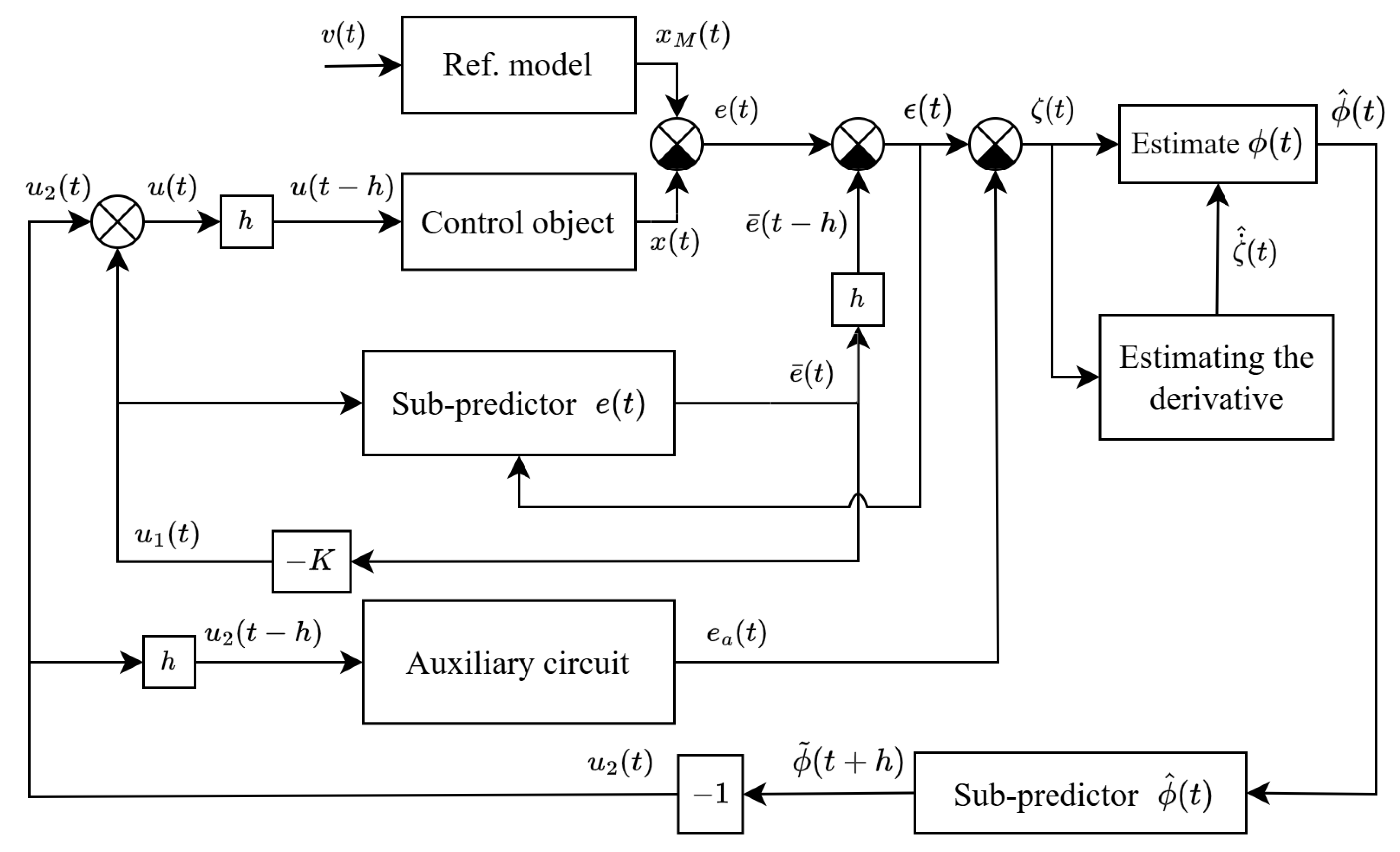In Section 3.2, we provide sufficient conditions for the stability of the closed-loop system in the form of solvable LMIs, using the Lyapunov–Krasovskii method and the S-procedure [26]. The proposed control scheme is depicted in Figure 1.

3.1. Design of the State Sub-Predictor and Disturbance Sub-Predictor

We introduce a state sub-predictor for the system (5) as follows:

$$\begin{array}{c}{\dot{\overline{e}}}_i\left(t\right)=A{\overline{e}}_i\left(t\right)+D_i\left({\overline{e}}_{i+1}\left(t\right)-{\overline{e}}_i(t-\overline{h})\right)+G\phi \left({\overline{e}}_i\left(t\right)\right)+B{u}_1(t-(i-1)\overline{h}),\hfill \\ {\dot{\overline{e}}}_q\left(t\right)=A{\overline{e}}_q\left(t\right)+D_q\left(e\left(t\right)-{\overline{e}}_q(t-\overline{h})\right)+G\phi \left({\overline{e}}_q\left(t\right)\right)+B{u}_1(t-(q-1)\overline{h}),\hfill \end{array}$$

(8)

where $i=1,\dots ,q,{\overline{e}}_i\left(t\right)\in {\mathbb{R}}^n$, and $\overline{h}={\displaystyle \frac{h}{q}}$. The integer $q>0$ is selected by the designer, and the matrices $D_i$ must be chosen such that the solutions of the following system are ultimately bounded:

$$\dot{\omega }\left(t\right)=\overline{A}\omega \left(t\right)-\overline{D}\omega (t-\overline{h}),$$

(9)

where $\omega \in {\mathbb{R}}^{nq}, \overline{A}=blkdiag\{A,q\}, \overline{D}=blkdiag\{D_1,\dots ,D_q\}$. The conditions for selecting the matrices $D_i$ in the form of an LMI are presented in Proposition 1.

Proposition 1.

If, for given matrices $D_i,i=1,\dots ,q$, there exist positive definite matrices $P=P^{\mathrm{T}}\in {\mathbb{R}}^{nq\times nq}$, $P_2\in {\mathbb{R}}^{nq\times nq}, P_3\in {\mathbb{R}}^{nq\times nq}, S=S^{\mathrm{T}}\in {\mathbb{R}}^{nq\times nq}, R=R^{\mathrm{T}}\in {\mathbb{R}}^{nq\times nq}$ such that the following LMI is feasible:

$$\left[\begin{array}{ccc}{\overline{A}}^{\mathrm{T}}{P}_2+P_2^{\mathrm{T}}\overline{A}+S-R& P-P_2^{\mathrm{T}}+{\overline{A}}^{\mathrm{T}}{P}_3& P_2^{\mathrm{T}}\overline{D}+R\\ ★& -P_3-P_3^{\mathrm{T}}+{\overline{h}}^{2}R& -P_3^{\mathrm{T}}\overline{D}\\ ★& ★& -S-R\end{array}\right]<0,$$

(10)

then ${\displaystyle \underset{t\to \infty }{lim}\omega \left(t\right)=0}$.

Proof. 

The proof of Proposition 1 is provided in Section 3.6.2 [26]. □

Remark 2.

Finding the matrices $D_i$ that satisfy the condition of Proposition 1 can be challenging in practice, particularly when the matrix A has a large dimension. Instead of defining the matrices $D_i$ directly and verifying the feasibility of LMI (10), one can assume $P_2,P_3$ as known matrices, for example, $P_2=P_3=I$, and then solve LMI (10) for $\overline{D},P,S,R$. The resulting matrices $D_i$ can then be used in the sub-predictor (8).

Remark 3.

By incrementally increasing the value of $\overline{h}$ and solving the LMI (10), one can determine the maximum value ${\overline{h}}_{max}$ for which LMI (10) admits a feasible solution for $D_i$. Based on this value, for a given input delay h, the required order q of the state sub-predictor can be determined as $q>{\displaystyle \frac{h}{\overline{h}}}$.

We introduce the following prediction errors:

$$\begin{array}{c}{ϵ}_i\left(t\right)={\overline{e}}_{i+1}(t-(q-i)\overline{h})-{\overline{e}}_i(t-(q-i+1)\overline{h}),i=1,\dots , q-1,\hfill \\ {ϵ}_q\left(t\right)=e\left(t\right)-{\overline{e}}_q(t-\overline{h}).\hfill \end{array}$$

(11)

By differentiating (11) with respect to the solutions obtained from Equations (5) and (8), we obtain

$$\begin{array}{ll}{\dot{ϵ}}_i\left(t\right)=& A{ϵ}_i\left(t\right)-D_i{ϵ}_i(t-\overline{h})+D_{i+1}{ϵ}_{i+1}(t-\overline{h})\\ & +G[\phi \left({\overline{e}}_{i+1}(t-(q-i)\overline{h})\right)-\phi \left({\overline{e}}_i(t-(q-i+1)\overline{h})\right)],i=1,\dots , q-1,\\ {\dot{ϵ}}_q\left(t\right)=& A{ϵ}_q\left(t\right)-D_q{ϵ}_q(t-\overline{h})+G[\phi \left(x\left(t\right)\right)-\phi \left({\overline{e}}_q(t-\overline{h})\right)]\\ & +B{u}_2(t-h)+B\varphi \left(t\right).\end{array}$$

(12)

To design the control signal $u_1\left(t\right)$, we assume that $\varphi \left(t\right)\equiv 0$ and $u_2\left(t\right)\equiv 0$. From Equation (11), we observe that ${\displaystyle \sum _{i=1}^q{ϵ}_i\left(t\right)=e\left(t\right)-{\overline{e}}_1(t-h)}$.

Thus, if system (12) is asymptotically stable, it follows that ${\displaystyle \underset{t\to \infty }{lim}e(t+h)=\underset{t\to \infty }{lim}{\overline{e}}_1\left(t\right)}$. Therefore, the control signal $u_1\left(t\right)$ is defined to ensure the stability of the closed-loop system in the following form:

$$u_1\left(t\right)=-K{\overline{e}}_1\left(t\right),$$

(13)

where the matrix K is selected such that the matrix $(A-BK)$ is Hurwitz.

However, in the presence of disturbances, we have $\varphi \not\equiv 0$. Therefore, it is essential to design the control signal $u_2\left(t\right)$ to reduce the influence of disturbances on the prediction errors ${ϵ}_i\left(t\right)$, for $i=1,\dots ,q$.

To achieve this, we introduce an auxiliary loop as follows:

$${\dot{e}}_a\left(t\right)=A{e}_a\left(t\right)-D_q{e}_a(t-\overline{h})+G[\phi \left(x\left(t\right)\right)-\phi \left({\overline{e}}_q(t-\overline{h})\right)]+B{u}_2(t-h),$$

(14)

where $e_a\left(t\right)\in {\mathbb{R}}^n$.

Let $\zeta \left(t\right)\triangleq {ϵ}_q\left(t\right)-e_a\left(t\right)$. From Equations (12) and (14), we obtain

$$\dot{\zeta }\left(t\right)=A\zeta \left(t\right)-D_q\zeta (t-\overline{h})+B\varphi \left(t\right).$$

(15)

From Equation (15), we derive the following equation for estimating the disturbance:

$$\widehat{\varphi }\left(t\right)=B^{+}\left(\widehat{\dot{\zeta }}\left(t\right)-A\zeta \left(t\right)+D_q\zeta (t-\overline{h})\right),$$

(16)

where the signal $\widehat{\dot{\zeta }}\left(t\right)$ is defined by the equation

$${\widehat{\dot{\zeta }}}_i\left(t\right)={\displaystyle \frac{p}{\mu p+1}}{\zeta }_i\left(t\right),i=1,\dots ,n.$$

(17)

Here, ${\zeta }_i$ and ${\widehat{\zeta }}_i$ are i-th element of the vectors $\zeta \left(t\right)$ and $\widehat{\zeta }\left(t\right)$, respectively. The parameter $\mu >0$ is a small positive number.

To predict the disturbance $\widehat{\varphi }(t+\widehat{h})$, we apply the method described in [22,23] as follows:

$$\widehat{\varphi }(t+\widehat{h})=\sum _{j=1}^{r+1}{(-1)}^{j-1}{C}_{r+1}^j\widehat{\varphi }(t-\widehat{h}(j-1))+\widehat{R}\left(t\right).$$

(18)

Here, $\widehat{h}={\displaystyle \frac{h}{M}}$, $M>0$ is an integer chosen by the designer and $\widehat{R}\left(t\right)={\widehat{h}}^{r+1}{\widehat{\varphi }}^{(r+1)}\left(t-\left[(r+1)\theta -1\right]\widehat{h}\right)$ represents the remaining part of the expansion. However, the value $\widehat{\varphi }(t+\widehat{h})$ alone is not sufficient to fully compensate for the disturbance. Therefore, we shift the argument of the function $\widehat{\varphi }(t+\widehat{h})$ in Equation (16) to the right by $\widehat{h}$, successively, M times. The resulting expression takes the following form:

$$\begin{array}{c}\tilde{\varphi }(t+\widehat{h})=\sum _{j=1}^{r+1}{(-1)}^{j-1}{C}_{r+1}^j\widehat{\varphi }(t-\widehat{h}(j-1)),\hfill \\ \tilde{\varphi }(t+l\widehat{h})=\sum _{j=1}^{l-1}{(-1)}^{j-1}{C}_{r+1}^j\tilde{\varphi }(t-\widehat{h}(j-l))+\sum _{j=l}^{r+1}{(-1)}^{j-1}{C}_{r+1}^j\widehat{\varphi }(t-\widehat{h}(j-l)),\hfill \\ l=2,\dots ,r(orl=2,\dots ,M,ifM<r+2),\hfill \\ \tilde{\varphi }(t+k\widehat{h})=\sum _{j=1}^{r+1}{(-1)}^{j-1}{C}_{r+1}^j\tilde{\varphi }(t-\widehat{h}(j-k)),\hfill \\ k=r+2,\dots ,M(ifM\ge r+2).\hfill \end{array}$$

(19)

From Equation (19), the prediction time is given by $\widehat{h}r={\displaystyle \frac{hr}{M}}$ for disturbance, indicating that the prediction time in (19) is reduced by a factor of M compared to the system delay. The system (19) is referred to as the disturbance sub-predictor, and M is the order of the disturbance sub-predictor.

After determining the predicted disturbance signal, we construct a control law for disturbance compensation in the following form:

$$u_2\left(t\right)=-\tilde{\varphi }(t+h).$$

(20)

Thus, we have developed a new control scheme that utilizes sub-predictors, including the control law (7), the sub-predictor of the controlled variable (8), the auxiliary feedback loop (14), and the disturbance sub-predictor (19). In the next subsection, we will analyze the closed-loop system to obtain the sufficient stability conditions.

3.2. Stability Analysis of the Closed-Loop System

Consider the estimation error $\xi =\dot{\zeta }-\widehat{\dot{\zeta }}$. Taking into account Equation (17), we obtain the derivative of $\dot{\xi }\left(t\right)$ as

$$\dot{\xi }\left(t\right)=-{\displaystyle \frac{1}{\mu }}\xi \left(t\right)+\ddot{\zeta }\left(t\right),$$

(21)

Differentiating Equation (15) twice and denoting $z=\ddot{\zeta }$, we obtain

$$\dot{z}\left(t\right)=Az\left(t\right)-D_{q}z(t-\overline{h})+B\ddot{\varphi }\left(t\right).$$

(22)

Since the signal $\ddot{\varphi }\left(t\right)$ is bounded and the matrix $D_q$ is chosen such that the solutions of Equation (9) are ultimately bounded, the signal $\xi \left(t\right)$ is also ultimately bounded. The new variables $\eta \left(t\right)={\xi }^{(r+1)}\left(t\right)$ and $g\left(t\right)={\zeta }^{(r+3)}\left(t\right)$ are then introduced. By differentiating the functions $\dot{\xi }\left(t\right)$ and $\dot{z}\left(t\right)$$(r+1)$ times, we obtain

$$\begin{array}{c}\dot{\eta }\left(t\right)=-{\displaystyle \frac{1}{\mu }}\eta \left(t\right)+g\left(t\right),\hfill \\ \dot{g}\left(t\right)=Ag\left(t\right)-D_{q}g(t-\overline{h})+B{\varphi }^{(r+3)}\left(t\right).\hfill \end{array}$$

(23)

Since the signal ${\varphi }^{(r+3)}\left(t\right)$ is bounded, the signal $\eta \left(t\right)$ is ultimately bounded as well. Let us rewrite Equation (15) as $\varphi \left(t\right)=B^{+}\left(\dot{\zeta }\left(t\right)-A\zeta \left(t\right)+D_q(t-\overline{h})\right)$. Considering Equations (16), (18)–(20), we derive the following relation:

$$\begin{array}{c}\lambda \left(t\right)=u_2(t-h)+\varphi \left(t\right)=\widehat{\varphi }\left(t\right)-\tilde{\varphi }\left(t\right)+\varphi \left(t\right)-\widehat{\varphi }\left(t\right)\hfill \\ =\widehat{\varphi }\left(t\right)-\tilde{\varphi }\left(t\right)+B^{+}\xi \left(t\right),\hfill \end{array}$$

(24)

Considering the structure of the disturbance sub-predictor in (18) and (19), the errors ${\epsilon }_l\left(t\right)\triangleq \widehat{\varphi }(t+l\widehat{h})-\tilde{\varphi }(t+l\widehat{h}),l=1,\dots ,M$ can be defined in the following form:

$$\begin{array}{c}{\epsilon }_1\left(t\right)=\widehat{R}\left(t\right),\hfill \\ {\epsilon }_l\left(t\right)=\sum _{j=1}^{l-1}{(-1)}^{j-1}{C}_{r+1}^j{\epsilon }_{l-j}\left(t\right)+{\epsilon }_1(t+(l-1)\widehat{h}),\hfill \\ l=2,\dots ,r+2(orl=2,\dots ,M,ifM\le r+2),\hfill \\ {\epsilon }_v\left(t\right)=\sum _{j=1}^{r+1}{(-1)}^{j-1}{C}_{r+1}^j{\epsilon }_{v-j}\left(t\right)+{\epsilon }_1(t+(v-1)\widehat{h}),\hfill \\ v=r+3,\dots ,M(ifM>r+2).\hfill \end{array}$$

(25)

Consequently, Equation (24) can be reformulated as follows:

$$\lambda \left(t\right)={\epsilon }_M(t-h)+B^{+}\xi \left(t\right).$$

(26)

The system described in Equation (12) can be rewritten in the following form:

$$\begin{array}{cc}\hfill {\dot{ϵ}}_i\left(t\right)& =A{ϵ}_i\left(t\right)-D_i{ϵ}_i(t-\overline{h})+D_{i+1}{ϵ}_{i+1}(t-\overline{h})\hfill \\ \hfill & +G\left[\phi \left({\overline{e}}_{i+1}(t-(q-i)\overline{h})\right)-\phi \left({\overline{e}}_i(t-(q-i+1)\overline{h})\right)\right],i=1,\dots ,q-1,\hfill \\ \hfill {\dot{ϵ}}_q\left(t\right)& =A{ϵ}_q\left(t\right)-D_q{ϵ}_q(t-\overline{h})+G\left[\phi \left(x\left(t\right)\right)-\phi \left({\overline{e}}_q(t-\overline{h})\right)\right]+B\lambda .\hfill \end{array}$$

(27)

Since $\xi \left(t\right)$ is bounded as shown earlier, we now aim to demonstrate that the signal $\lambda \left(t\right)$ is also bounded. To achieve this, we first show that the prediction error ${\epsilon }_M\left(t\right)$ is bounded.

Differentiating Equation (15) yields

$$\ddot{\zeta }\left(t\right)=A\dot{\zeta }\left(t\right)-D_q\dot{\zeta }(t-\overline{h})+B\dot{\varphi }\left(t\right).$$

Since $\dot{\varphi }\left(t\right)$ is bounded, it follows that $\dot{\zeta }\left(t\right)$ is also bounded.

Next, Equation (17) can be rewritten as

$$\dot{\widehat{\dot{\zeta }}}\left(t\right)=-{\displaystyle \frac{1}{\mu }}\widehat{\dot{\zeta }}\left(t\right)+{\displaystyle \frac{1}{\mu }}\dot{\zeta }\left(t\right),$$

which, combined with the boundedness of $\dot{\zeta }\left(t\right)$, implies that $\widehat{\dot{\zeta }}\left(t\right)$ is bounded.

Considering Equation (16), and noting that both $\widehat{\dot{\zeta }}\left(t\right)$ and $\zeta \left(t\right)$ are bounded, we conclude that $\widehat{\varphi }\left(t\right)$ is also bounded. Furthermore, since $\widehat{\varphi }\left(t\right)$ is bounded and Equation (19) holds, it follows that $\tilde{\varphi }\left(t\right)$ is bounded.

As a result, the prediction error ${\epsilon }_M\left(t\right)$ is bounded, and consequently, the signal $\lambda \left(t\right)$ is also bounded.

We introduce a new variable ${\displaystyle x_e\left(t\right)\triangleq {\overline{e}}_1(t-h)=e\left(t\right)-\sum _{i=1}^q{ϵ}_i\left(t\right)}$. From Equations (1) and (9), we obtain the derivative of $x_e\left(t\right)$ with respect to time as follows:

$${\dot{x}}_e\left(t\right)=(A-BK)x_e\left(t\right)+D_1{ϵ}_1(t-\overline{h})+G\phi \left(x_e\left(t\right)\right).$$

(28)

Since the solutions of Equations (21)–(23) are ultimately bounded, we now focus on studying the ISS of the closed-loop system by considering only Equations (27), (28), and (2). To proceed, we define the following vectors and matrices:

$$\begin{array}{c}{x}_p=col\left\{x_e,{ϵ}_1,{ϵ}_2,\dots ,{ϵ}_q,x_M\right\},\mathsf{\Lambda }=col\{\lambda ,\nu \},\hfill \\ \psi \left(t\right)=col\{\phi \left(x_e\left(t\right)\right),\phi \left({\overline{e}}_{i+1}(t-(q-i)\overline{h})\right)-\phi \left({\overline{e}}_i(t-(q-i+1)\overline{h})\right),\hfill \\ \phi (x\left(t\right)-\phi \left({\overline{e}}_q(t-h)\right)\},i=1,\dots ,q-1,\hfill \\ A_p=blkdiag\{A-BK,blkdiag\{A,q\},A_M\},\hfill \\ B_p=\left[\begin{array}{cc}0& 0\\ ⋮& ⋮\\ 0& 0\\ B& 0\\ 0& B\end{array}\right],C_p=\left[\begin{array}{c}blkdiag\{G,q+1\}\\ 0\end{array}\right]\hfill \\ D_p=\left[\begin{array}{cccccc}0& D_1& 0& 0& \dots & 0\\ 0& -D_1& D_2& 0& \dots & 0\\ 0& 0& -D_2& D_3& \dots .& 0\\ 0& 0& 0& -D_3& \dots & 0\\ ⋮& ⋮& ⋮& ⋮& \ddots & ⋮\\ 0& 0& 0& 0& \dots & -D_q\\ 0& 0& 0& 0& \dots & 0\end{array}\right].\hfill \end{array}$$

Using the notations defined above, Equations (2), (27), and (28) can be rewritten as follows:

$${\dot{x}}_p\left(t\right)=A_p{x}_p\left(t\right)+D_p{x}_p(t-\overline{h})+B_p\mathsf{\Lambda }\left(t\right)+C_p\psi \left(t\right).$$

(29)

By applying the Newton–Leibniz formula, (29) can be rewritten as

$${\dot{x}}_p\left(t\right)=\left(A_p+D_p\right)x_p\left(t\right)-D_p{\int }_{t-\overline{h}}^t{\dot{x}}_p\left(s\right)ds+B_p\mathsf{\Lambda }\left(t\right)+C_p\psi \left(t\right).$$

(30)

Theorem 1.

Consider the nonlinear system (1), the reference model (2), the sub-predictor for the controlled variable (8), the disturbance sub-predictor (19), and the control law (7). Suppose that for a given number $\alpha >0$ and matrices K and $D_p$, there exist coefficients $\beta >0,\gamma >0$ and positive-definite matrices $P>0,P_2>0,P_3>0,Q>0,S>0$ such that the following LMI is feasible:

$$\mathsf{\Psi }:=\left[\begin{array}{cccccc}{\mathsf{\Psi }}_{11}& {\mathsf{\Psi }}_{12}& 0& -\overline{h}{P}_2^{\mathrm{T}}{D}_p& P_2^{\mathrm{T}}{B}_p& P_2^{\mathrm{T}}{C}_p\\ ★& {\mathsf{\Psi }}_{22}& 0& -\overline{h}{P}_3^{\mathrm{T}}{D}_p& P_3^{\mathrm{T}}{B}_p& P_3^{\mathrm{T}}{C}_p\\ ★& ★& -e^{-2\alpha \overline{h}}Q& 0& 0& 0\\ ★& ★& ★& -\overline{h}S& 0& 0\\ ★& ★& ★& ★& -\gamma I& 0\\ ★& ★& ★& ★& ★& -\beta I\end{array}\right]\le 0.$$

(31)

where

$$\begin{array}{c}{\mathsf{\Psi }}_{11}=P_2^T(A_p+D_p)+{(A_p+D_p)}^T{P}_2+2\alpha P+Q+\beta L^{2}I,\hfill \\ {\mathsf{\Psi }}_{12}=P-P_2^{\mathrm{T}}+{(A_p+D_p)}^{\mathrm{T}}{P}_3,\hfill \\ {\mathsf{\Psi }}_{22}=-P_3-P_3^{\mathrm{T}}+\overline{h}S.\hfill \end{array}$$

Then, the solutions of the closed-loop system defined by (1), (2), (7), (8), (13), (14) and (16)–(20) are ultimately bounded. Moreover, the objective (6) holds with $\delta =\mathrm{O}\left({\left({\displaystyle \frac{h}{M}}\right)}^{r+1}{\displaystyle \underset{t\to \infty }{\overline{lim}}}\left|{\varphi }^{(r+1)}\left(t\right)\right|\right)$.

Proof. 

Consider the Lyapunov–Krasovskii candidate function in the following form:

$$V=V_1+V_2+V_3$$

(32)

where

$$V_1=x_p^{T}P{x}_p,V_2={\int }_{t-\overline{h}}^t{e}^{2\alpha (\sigma -t)}{x}_p^{\mathrm{T}}\left(\sigma \right)Q{x}_p\left(\sigma \right)d\sigma ,$$

$$V_3={\int }_{-\overline{h}}^0{\int }_{t+\tau }^t{e}^{2\alpha (\sigma -t)}{\dot{x}}_p^{\mathrm{T}}\left(\sigma \right)S{\dot{x}}_p\left(\sigma \right)d\sigma d\tau .$$

It is important to note that the component $V_3$ enables us to derive the stability condition for the closed-loop system, which will explicitly depend on the delay (a delay-dependent condition, as outlined in [26]. Based on Equation (30), we proceed to derive the following expressions:

$$\begin{array}{cc}\hfill {\dot{V}}_1+2\alpha V_1& =x_p^{\mathrm{T}}\left(t\right)P{\dot{x}}_p\left(t\right)+2\alpha x_p^{\mathrm{T}}\left(t\right)P{x}_p\left(t\right)+2\left[x_p^{\mathrm{T}}\left(t\right)P_2^{\mathrm{T}}+{\dot{x}}_p^{\mathrm{T}}\left(t\right)P_3^{\mathrm{T}}\right]\times \hfill \\ \hfill & \times \left[\left(A_p+D_p\right)x_p\left(t\right)-D{\int }_{t-\overline{h}}^{\mathrm{T}}{\dot{x}}_p\left(s\right)ds+B_p\mathsf{\Lambda }\left(t\right)+C_p\psi \left(t\right)-{\dot{x}}_p\left(t\right)\right],\hfill \\ \hfill {\dot{V}}_2+2\alpha V_2& =x_p^{\mathrm{T}}\left(t\right)Q{x}_p\left(t\right)-e^{-2\alpha \overline{h}}{x}_p^{\mathrm{T}}(t-\overline{h})Q{x}_p(t-\overline{h}),\hfill \\ \hfill {\dot{V}}_3+2\alpha V_3& =\overline{h}{\dot{x}}_p^{\mathrm{T}}\left(t\right)S{\dot{x}}_p\left(t\right)-{\int }_{t-\overline{h}}^{\mathrm{T}}{e}^{2\alpha (\sigma -t)}{\dot{x}}_p^{\mathrm{T}}\left(\sigma \right)S{\dot{x}}_p\left(\sigma \right)d\sigma .\hfill \end{array}$$

(33)

The first expression in (33) is derived using the descriptor method from [26]. By applying Jensen’s inequality [26], we can estimate the last expression in (33) as follows:

$${\dot{V}}_3+2\alpha V_3⩽h{\dot{x}}_p^{\mathrm{T}}\left(t\right)S{\dot{x}}_p\left(t\right)-{\displaystyle \frac{e^{-2\alpha h}}{h}}{\int }_{t-h}^{\mathrm{T}}{\dot{x}}_p^{\mathrm{T}}\left(\sigma \right)d\sigma S{\int }_{t-h}^{\mathrm{T}}{\dot{x}}_p\left(\sigma \right)d\sigma ,$$

(34)

Considering the Lipschitz condition of function $\phi (·)$, we obtain

$$\begin{array}{c}{\displaystyle {\psi }^{\mathrm{T}}\psi \le {\left[\phi \left(x_e\left(t\right)\right)\right]}^2+\sum _{i=1}^{q-1}{\left[\phi \left({\overline{e}}_{i+1}(t-(q-i)\overline{h})\right)-\phi \left({\overline{e}}_i(t-(q-i+1)\overline{h})\right)\right]}^2}\hfill \\ +{\left[\phi \left(x\left(t\right)\right)-\phi ({\overline{e}}_q(t-\overline{h})\right]}^2\le L^2\left({\displaystyle x_e^2+\sum _{i=1}^{q-1}{ϵ}_i^2+{(x\left(t\right)-{\overline{e}}_q(t-\overline{h}))}^2}\right)\hfill \\ =L^2\left({\displaystyle x_e^2\left(t\right)+\sum _{i=1}^{q-1}{ϵ}_i^2\left(t\right)+{(x_M\left(t\right)+e\left(t\right)-{\overline{e}}_q(t-\overline{h}))}^2}\right)\hfill \\ \le L^2\left({\displaystyle x_e^2\left(t\right)+\sum _{i=1}^q{ϵ}_i^2\left(t\right)+x_M^2\left(t\right)}\right)\le L^2{x}_p^{\mathrm{T}}{x}_p.\hfill \end{array}$$

(35)

By defining $y\left(t\right)=col\{x_p\left(t\right),{\dot{x}}_p\left(t\right),x_p(t-h),{\displaystyle \frac{1}{h}}{\int }_{t-h}^{\mathrm{T}}{\dot{x}}_p\left(\sigma \right)d\sigma ,\mathsf{\Lambda }\left(t\right),\psi \left(t\right)\}$ and applying the S-procedure, we present the following expression for studying the ISS properties:

$$\dot{V}+2\alpha V+\beta \left(L^2{x}_p^{\mathrm{T}}{x}_p-{\psi }^{\mathrm{T}}\psi \right)-\gamma {\lambda }^{\mathrm{T}}\lambda ⩽y^{\mathrm{T}}\mathsf{\Psi }y.$$

(36)

If the condition (31) holds, then $y^{\mathrm{T}}\mathsf{\Psi }y\le 0$, which implies that $\dot{V}+2\alpha V\le \gamma {\lambda }^{\mathrm{T}}\lambda$ for all $x_p\in {\mathbb{R}}^{2n+nq}$ where the Lipschitz condition of function $\phi (·)$ is satisfied. Consequently, $x_p\left(t\right)$ is ultimately bounded.

Consider the control objective (6). Based on Equations (7) and (24), we can rewrite Equation (5) as $\dot{e}\left(t\right)=Ae\left(t\right)+G\phi \left(x\left(t\right)\right)+B{u}_1(t-h)+B\lambda \left(t\right)$. If $\lambda \equiv 0$, then according to (36), we obtain the exponential stable closed-loop system. Denote $\mathsf{\Delta }\left(\mu \right):={\overline{lim}}_{t\to \infty }\left|\lambda \left(t\right)\right|$. Taking into account (21) and (26), we have

$$\underset{\mu \to 0}{lim}\mathsf{\Delta }\left(\mu \right)=\underset{t\to \infty }{\overline{lim}}\left|{\epsilon }_M\left(t\right)\right|.$$

(37)

As a result, the proposed algorithm provides objective (6) with the accuracy $\delta =\mathrm{O}\left({\displaystyle \underset{t\to \infty }{\overline{lim}}}\left|{\epsilon }_M\left(t\right)\right|\right)$.

We now show that ${\displaystyle \underset{t\to \infty }{\overline{lim}}}\left|{\epsilon }_M\left(t\right)\right|=\mathrm{O}\left({\left({\displaystyle \frac{h}{M}}\right)}^{r+1}{\displaystyle \underset{t\to \infty }{\overline{lim}}}\left|{\varphi }^{(r+1)}\left(t\right)\right|\right)$. Indeed, taking into account (25) and (18), we obtain

$$\underset{t\to \infty }{\overline{lim}}\left|{\epsilon }_M\left(t\right)\right|=\mathrm{O}\left(\underset{t\to \infty }{\overline{lim}}\left|\widehat{R}\left(t\right)\right|\right).$$

(38)

According to (15)–(17) and (21)–(23), the expression for $\widehat{R}\left(t\right)$ can be written as

$$\begin{array}{cc}\hfill \widehat{R}\left(t\right)& ={\widehat{h}}^{r+1}[{\varphi }^{(r+1)}\left(t-\left[(r+1)\theta -1\right]\widehat{h}\right)\hfill \\ \hfill & -\left({\varphi }^{(r+1)}\left(t-\left[(r+1)\theta -1\right]\widehat{h}\right)-{\widehat{\varphi }}^{(r+1)}\left(t-\left[(r+1)\theta -1\right]\widehat{h}\right)\right)]\hfill \\ \hfill & ={\widehat{h}}^{r+1}\left[{\varphi }^{(r+1)}\left(t-\left[(r+1)\theta -1\right]\widehat{h}\right)-B^{+}\eta \left(t-\left[(r+1)\theta -1\right]\widehat{h}\right)\right]\hfill \end{array}$$

(39)

Since $\eta \left(t\right)\to 0$ as $\mu \to 0$, we obtain

$$\delta =\mathrm{O}\left({\left({\displaystyle \frac{h}{M}}\right)}^{r+1}\underset{t\to \infty }{\overline{lim}}\left|{\varphi }^{(r+1)}\left(t\right)\right|\right).$$

Theorem 1 is proved. □

Remark 4.

We now demonstrate the boundedness of all signals in the closed-loop system. Since $x_p\left(t\right)$ is bounded, it follows that $x_e\left(t\right)$, ${ϵ}_i\left(t\right)$, and $e\left(t\right)$ are also bounded. From Equation (11), it can be concluded that the state ${\overline{e}}_i\left(t\right)$ of the sub-predictor (8) is bounded as well. As a result, the control signal $u_1\left(t\right)$ remains bounded. Moreover, because $\tilde{\varphi }\left(t\right)$ is bounded, $u_2\left(t\right)$ is bounded as well. Therefore, all signals in the closed-loop system remain bounded.

4. Numerical Example

Let us consider the model of a single link robot with a flexible joint rotating in a vertical plane with the following parameters [27]:

$$\begin{gathered} A=\left[\begin{array}{cccc}0& 1& 0& 0\\ -{\displaystyle \frac{k}{J_1}}& 0& {\displaystyle \frac{k}{J_1}}& 0\\ 0& 0& 0& 1\\ {\displaystyle \frac{k}{J_2}}& 0& -{\displaystyle \frac{k}{J_2}}& 0\end{array}\right], B=F=\left[\begin{array}{c}0\\ 0\\ 0\\ {\displaystyle \frac{1}{J_2}}\end{array}\right], G=\left[\begin{array}{cccc}0& 0& 0& 0\\ -{\displaystyle \frac{mgl}{J_1}}& 0& 0& 0\\ 0& 0& 0& 0\\ 0& 0& 0& 0\end{array}\right], \\ \phi \left(x\left(t\right)\right)=sinx\left(t\right),x_0={\left[\begin{array}{cccc}0.1& 0& 0.1& 0\end{array}\right]}^{\mathrm{T}}, \end{gathered}$$

where $x=col\{x_1,x_2,x_3,x_4\}\in {\mathbb{R}}^4$; $x_1$ and $x_2$ are the link displacement [m] and velocity [m/s], respectively; $x_3$ and $x_4$ are the rotor displacement [rad] and angular velocity [rad/s], respectively. The parameters $J_1,J_2,k,l,$ and g are the link inertia, the rotor inertia, the elastic constant, the position of the center of mass, and the gravity acceleration, respectively. These parameters are given as $J_1=J_2=10{\mathrm{Kg}/\mathrm{m}}^2,k=1\mathrm{N}/\mathrm{m},l=0.5\mathrm{m},g=9.8{\mathrm{m}/\mathrm{s}}^2,$ $m=0.1\mathrm{Kg}$. The Lipschitz constant is assumed to be equal to 0.3691.

Consider the disturbance $f\left(t\right)$ in the following form:

$$f\left(t\right)=1+sin\left(0.2t\right)+cos\left(0.3t\right)+sin(0.05t+{\displaystyle \frac{\pi }{4}})+{\displaystyle \frac{100}{{(5p+1)}^7}}sat\left({\displaystyle \frac{d\left(t\right)}{10}}\right),$$

where $sat(·)$ is the saturation function, $d\left(t\right)$ is the signal modeled in the Matlab Simulink environment (latest v. R2025a) using the “Band-Limited White Noise” block with a noise power of $0.1$ and a sample time of $0.1$.

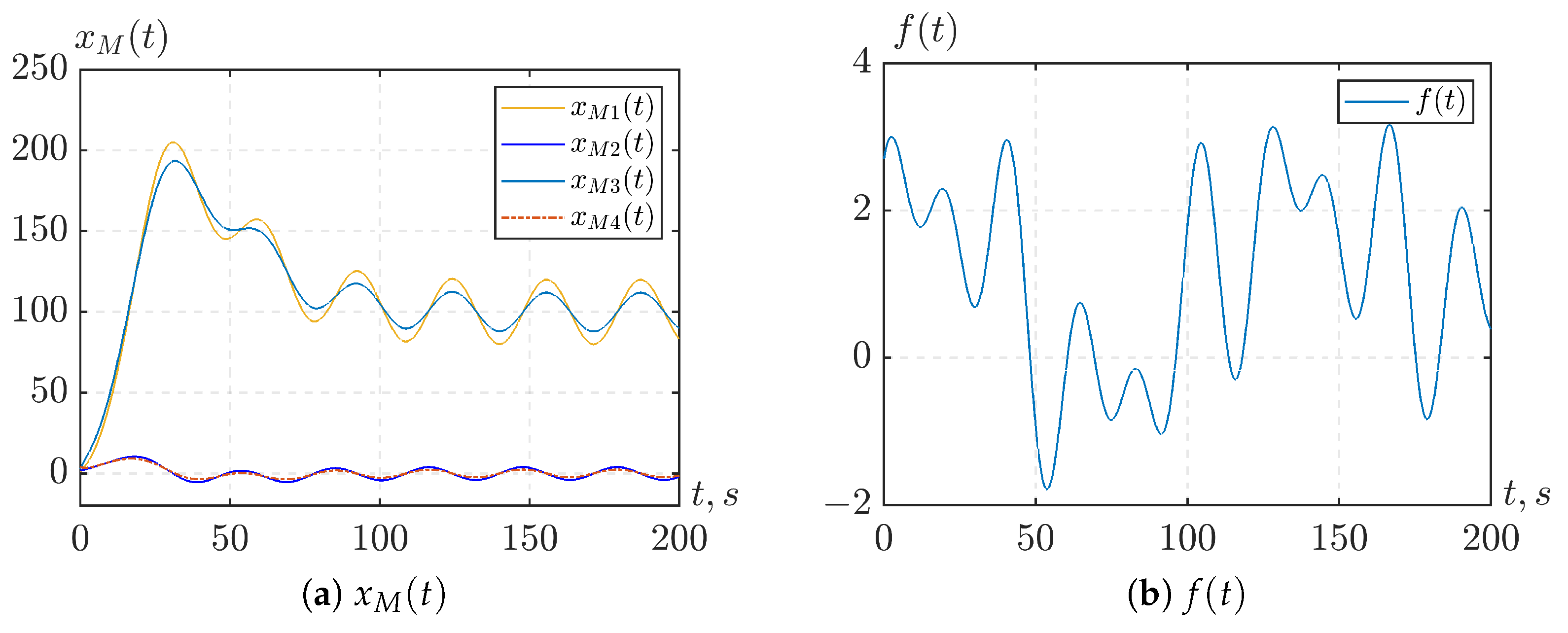
The matrix $A_M$ of the reference model is given by $A_M=A-B{c}_1$, where $c_1$ is computed using the MATLAB command $c_1=acker(A,B,[-0.1,-0.1,-0.1,-0.1])$. The reference signal is given by $\nu =1+5sin\left(0.2t\right)$. The graphs of the state of the reference model $x_M\left(t\right)$ and the disturbance $f\left(t\right)$ are illustrated in Figure 2.

Let us select $q=2$ for the state sub-predictor. Let $P_1=P_2=I\in {\mathbb{R}}^4$; it is shown that the LMI in Equation (10) is solvable for the variables $D_1$, $D_2$, P, R, and S when $\overline{h}\le 1.2$ s. For $\overline{h}=1.2$ s, we obtain

$$D_1=D_2=D_{\overline{h}max}=\left[\begin{array}{cccc}0.5449& 0.2551& 0.0110& -0.0013\\ -0.1139& 0.4665& 0.0177& 0.0044\\ 0.0110& -0.0013& 0.5449& 0.2551\\ 0.0177& 0.0044& -0.1139& 0.4665\end{array}\right].$$

Since the LMI (10) is convex with respect to $\overline{h}$, the system (1) remains stable for $\overline{h}\in [0,1.2]$, which means $h\in [0,2.4]$ when using the found matrix $D_{\overline{h}max}$ [26]. Using the command acker in MATLAB to calculate the gain K such that the eigenvalues of the closed-loop system are $\{-16,-12,-8,-2\}$, we obtain $K=[302321,236419,4877,380]$. Checking the feasibility of the LMI (31), we find that (31) is feasible for $\overline{h}\le {\overline{h}}_{max}=1.2$ s.

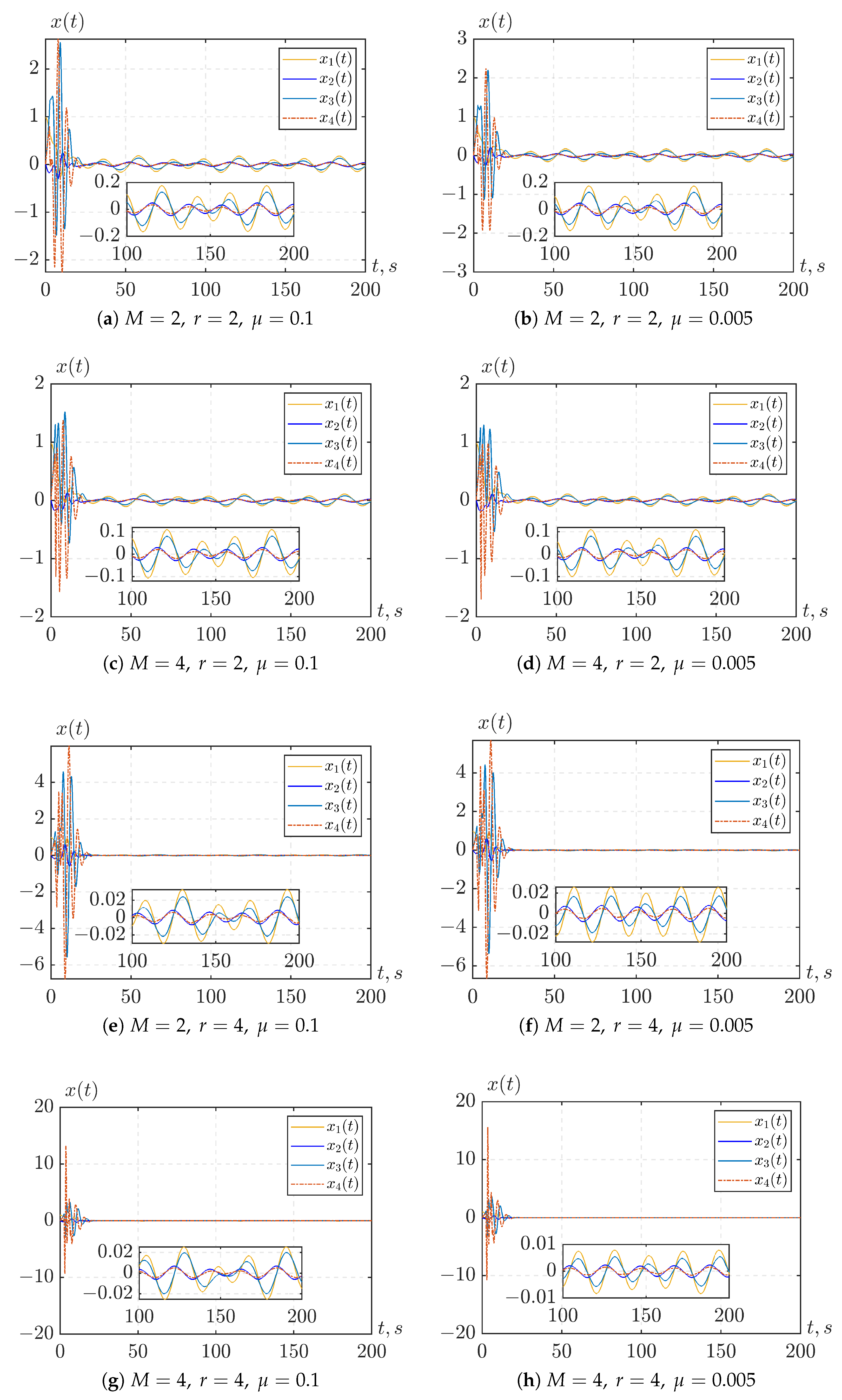
To illustrate the control performance, we consider the simulation results where the parameters M, r, and $\mu$ are selected from the set $\left\{M=(2,4),r=(2,4),\mu =(0.005,0.1)\right\}$.

Figure 3 illustrates the case of stabilization of the system state vector $x\left(t\right)$ when the input to the reference model is identically zero, i.e., $\nu \left(t\right)\equiv 0$, and the time delay is set to $h=h_{max}=2.4$ s. From the graphs, we can make the following observations:

• All controlled signals $x\left(t\right)$ are ultimately bounded with some bound $\delta$.
• The bound $\delta$ decreases as either M or r increases, or as both increase simultaneously. This is consistent with the conclusion above that the magnitude of $\delta$ depends on ${\left({\displaystyle \frac{h}{M}}\right)}^{r+1}{\displaystyle \underset{t\to \infty }{\overline{lim}}}\left|{\varphi }^{(r+1)}\left(t\right)\right|$.
  For example, in the case of a given disturbance $f\left(t\right)$ whose higher-order derivatives decrease in magnitude (see Assumption 3), increasing M from 2 to 4 (with fixed r) reduces $\delta$ by approximately a factor of 2, except for the case with $\mu =0.1$ and $r=4$ (see Figure 3e,g), which will be discussed below. On the other hand, when M is fixed and r is increased from 2 to 4, $\delta$ decreases by approximately a factor of 10. In the case with $\mu =0.1,M=4$, the reduction is less significant, with $\delta$ decreasing by approximately a factor of 5 (see Figure 3c,g).
  However, increasing M or r to reduce $\delta$ may lead to a larger overshoot in the controlled signals, especially when increasing M with a large r (see Figure 3e–h). This behavior can be explained by the structure of the disturbance sub-predictor, which contains coefficients dependent on M and r. When both M and r are large, the disturbance sub-predictor may produce large transient prediction errors, which in turn cause significant overshoots in the controlled signals.
• A smaller value of $\mu$ (e.g., $\mu =0.005$) provides better control performance compared to a larger value (e.g., $\mu =0.1$). This explains why, for $r=4$, increasing M does not reduce $\delta$ when $\mu =0.1$ is selected (see Figure 3e,g). A similar pattern is observed in Figure 3c,g, where increasing r results in a smaller reduction in $\delta$ compared to the case with a smaller $\mu$.
  When $\mu =0.005$ is used, increasing either M or r leads to a significant reduction in $\delta$. This is because the “dirty derivative” filters in (17) yield a more accurate derivative estimation when $\mu$ is smaller.

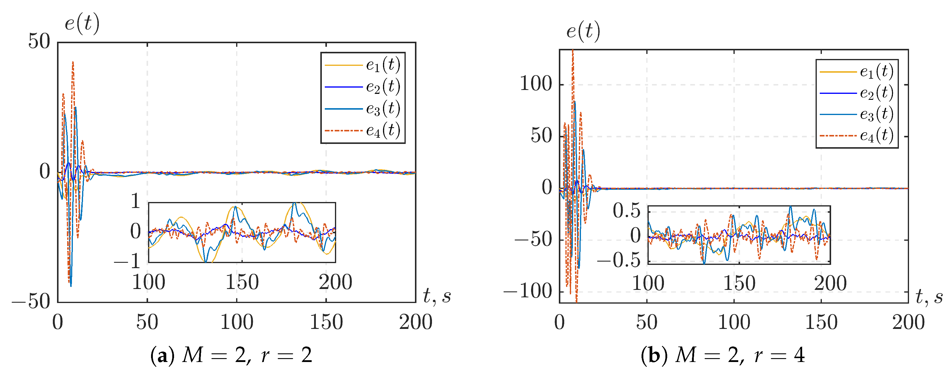
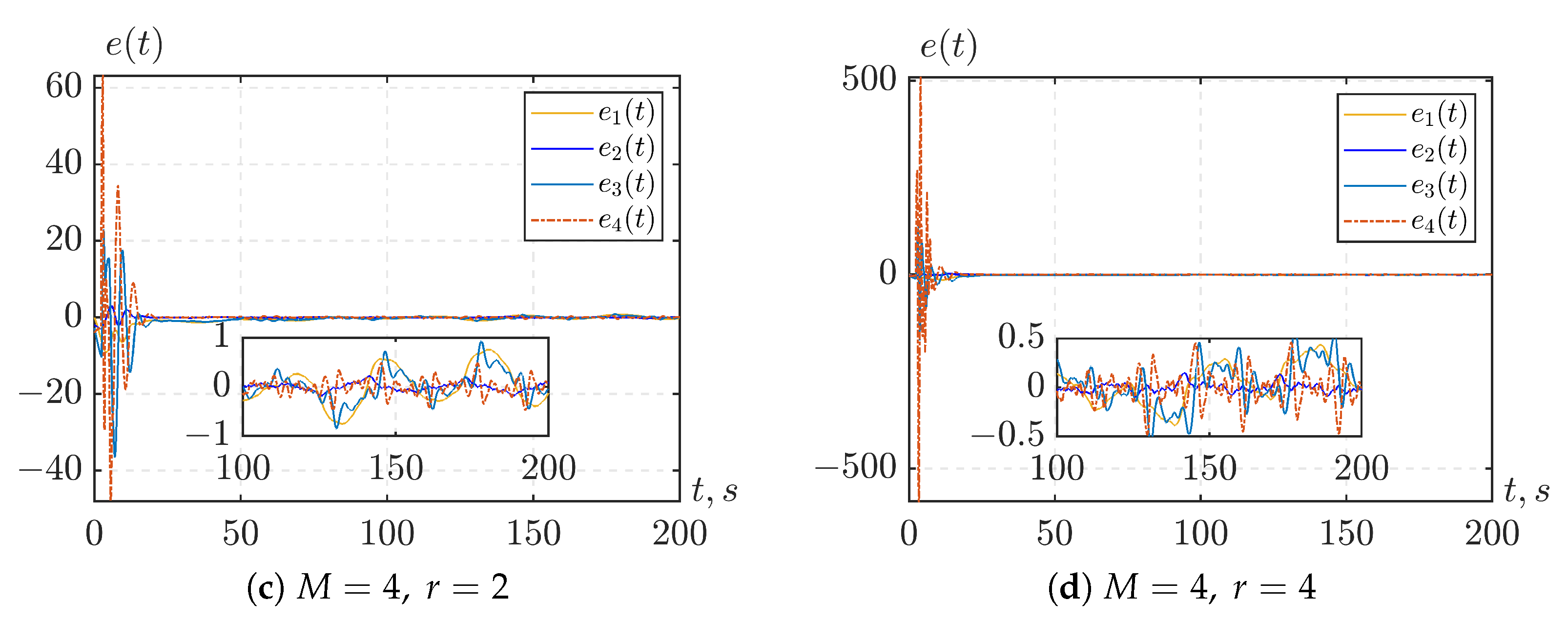
Figure 4 illustrates the case of stabilization of the tracking error $e\left(t\right)$ when the time delay is set to $h=h_{max}=2.4$ s and $\mu =0.005$. From the graphs, we observe that increasing the value of M can reduce $\delta$; however, the effect is not as significant as when increasing the value of r. This can be explained by the fact that the bound $\delta$ depends on the magnitude of the disturbance $\varphi \left(t\right)$, which is a function of $f\left(t\right)$, $x_M\left(t\right)$, and $\nu \left(t\right)$, and these terms can attain large values. However, increasing both r and M leads to large peak values during the transient regime, as previously observed in the case of system state stabilization.

5. Conclusions

In this paper, a novel control law is proposed for nonlinear systems with constant input delays. The control strategy employs sub-predictors for both the controlled variables and the external disturbances. By applying the Lyapunov–Krasovskii functional method, sufficient conditions for the stability of the closed-loop nonlinear system are derived in terms of linear matrix inequality (LMI) feasibility. The effectiveness of the proposed algorithm is demonstrated through simulation results. It is shown that the tracking (or stabilization) error converges to a neighborhood of zero with accuracy $\delta$, which depends on the magnitude of the disturbances. Moreover, increasing the order of the disturbance sub-predictor can improve the accuracy $\delta$, although it may result in a larger peak in the transient response.