1. Introduction
If a binary dataset with the responses of
and 1 has excess zeros, the dataset is zero-inflated. The zero-inflated Bernoulli, denoted by ZIBer, model can be used to characterize binary zero-inflated datasets. The excess zeros can be structural or chance zeros. A structural zero means that the zeros are caused by inherent constraints or conditions. Other than structural zeros, the response variable
Y follows a Bernoulli distribution, in which
with a probability
and
with the probability
. Diop et al. [
1] provided a medical example. Assume that the infection response is related to some diseases.
means an infected individual and
otherwise. An immunity agent can control if the individual is infected; that is, the individual is immune and labeled by
if the individual cannot be infected. See Ridout et al. [
2] for more discussions about structural and chance zeros. The ZIBer model has been suggested for modeling zero-inflated datasets, with its superiority over the logistic model. To save pages, abbreviations in
Table 1 are used in this study so that the readers can follow the arguments.
Today, datasets with a highly disproportionate distribution of categories can be seen occasionally. Such datasets are called imbalanced data in machine learning analysis. The ZIBer model can be an alternative to characterize imbalanced datasets, see Chiang et al. [
3] and Xin et al. [
4].
Lambert [
5] was a pioneer in using the zero-inflated model with the Poisson distribution, named the ZIP model. He used the logit function to link the probability of response
and covariates. Moreover, the maximum likelihood estimation method was used for making statistical inferences. The ZIP model addresses random events that include an abundance of zero-count data within a given time frame. The ZIP model combines two processes that produce zeros. The first process is responsible for generating zeros, while the second process, guided by a Poisson distribution, produces counts. After that, the ZIP model has earned more attention. However, Lambert [
5] mentioned that the ZIP model has the drawback of over-dispersion inherited from the Poisson model. To overcome this drawback, he also proposed the zero-inflated negative Binomial model. The zero-inflated model was also extended to the Binomial distribution, see [
6,
7,
8,
9,
10,
11] for more comprehensive discussions. Recent studies about using zero-inflated models for characterizing binary responses have been conducted by [
12,
13,
14,
15,
16].
Compared with the ZIP, zero-inflated negative Binomial, and zero-inflated Binomial models, fewer existing studies have paid attention to the binary classification for zero-inflated datasets. Dio et al. [
1] proposed a simulation-based inference method for binary responses with zero-inflated datasets. Chiang et al. [
3] proposed an expectation–maximization (EM) algorithm to obtain reliable maximum likelihood estimates of the ZIBer parameters and named it EM-ZIBer. Considering an overfitting penalty for the ZIBer model, Xin et al. [
4] developed a modeling process by using elastic net regularization (ENR) to prohibit model overfitting and named the model the ENR-ZIBer model. The sensitivity of the method proposed by Xin et al. [
4] is still lower and unsatisfactory. There is room to improve the performance of the estimation method provided by Xin et al. [
4] to that of the ZIBer model for zero-inflated datasets.
The zero-inflated structure is a crucial factor in making the data imbalanced. The ENR-ZIBer model outperforms the logistic model in characterizing zero-inflated datasets. However, there is room to enhance the performance of the ENR-ZIBer model for characterizing imbalanced datasets or keeping a high performance if the model contains many explanatory variables. Using the regularization rule can force the ENR-ZIBer model to screen out less important explanatory variables. However, the regularization rule also increases the possibility of not obtaining reliable model estimates. For more information, readers are suggested to refer to Xin et al. [
4].
For zero-inflated datasets, Chiang et al. [
3] showed that the EM-ZIBer model is competitive with other weak learners, for example, the light gradient boosting machine and artificial neural network methods. Xin et al. [
4] showed the superiority of the ENR-ZIBer model over the EM-ZIBer model proposed by Chiang et al. [
3] and the logistic model. However, the ENR-ZIBer model in Xin et al. [
4] failed due to the covariates of the latent variable being difficult to identify. Moreover, Xin et al. [
4] did not study the performance of the ENR-ZIBer model with data augmentation. To enhance the classification performance of the ENR-ZIBer model for zero-inflated data, machine learning algorithms could have the potential to beat the gradient descent method using the momentum learning rate, labeled as GDM-Mom, proposed by Xin et al. [
4]. By the way, if the data are zero-inflated, it could make the data imbalanced. The performance of the ENR-ZIBer model needs to be verified.
Kennedy and Eberhart [
17] first proposed the particle swarm optimization (PSO) method in 1995. Inspired by the collective behavior of fish schooling and birds flocking, the PSO is a population-based metaheuristic algorithm for optimization problems by iteratively updating a swarm of particles or candidate solutions. The PSO algorithm is effective for continuous optimization problems and can be implemented with a few hyperparameters. Wang [
18] used the multi-kernel functions to improve Fuzzy C-Means, named MK-FCM, and then improve the performance of the PSO method.
In machine learning applications for binary-response data, the synthesized minority oversampling technique, denoted by SMOTE, is a popular method for data augmentation to deal with imbalanced data. The augmented data are then used to train the model for binary classification. When the positive class is under-represented, standard classifiers could perform biased classification on the majority class and lead to poor detection of the minority class. SMOTE is particularly effective when used in combination with ensemble methods or resampling techniques. Dablain et al. [
19] proposed a novel oversampling algorithm, named DeepSMOTE, for deep learning models. Integrating the geometric SMOTE method and the SMOTE method for Nominal and Continuous features, Fonseca et al. [
20] proposed a geometric SMOTE method for Nominal and Continuous features, named the G-SMOTENC method. G-SMOTENC is an oversampling method to reach a significant improvement in classification performance. Elreedy et al. [
21] derived the mathematical formulation for the probability distribution of generated samples using the SMOTE method. More applications using different SMOTE methods can be found in [
22,
23,
24,
25,
26,
27,
28,
29]. To the best of the authors’ knowledge, using the SMOTE method to enhance the performance of the ENR-ZIBer model is an open issue and must be verified.
The methods of Xin et al. [
4] have three weaknesses:
- 1.
The ENR-ZIBer model used by Xin et al. [
4] will fail if the covariates of the latent variable cannot be clearly identified. We suggest using an unknown proportion parameter to replace the second logit model used by Xin et al. [
4] to enhance the performance of the ENR-ZIBer model.
- 2.
The GDM-Mom method proposed by Xin et al. [
4] has room to be improved to obtain reliable parameter estimates.
- 3.
Xin et al. [
4] did not evaluate the effect of data augmentation for the ENR-ZIBer model. SMOTE is a popular technique for data augmentation in machine learning applications. It is important to check if SMOTE can enhance the predictive performance of the ENR-ZIBer model.
To validate the quality of the competitive models used in this study, three popular methods for the cross-validation of machine learning models are considered. They are the holdout cross-validation, leave-one-out cross-validation, and K-fold cross-validation methods. In the holdout cross-validation method, a sample is randomly split into a training and test sample. It is common to keep a large proportion of the observations in the sample for the training sample and use the other observations for the test sample. Leave-one-out cross-validation keeps the hth observation for testing and uses the other for the training sample to train the machine learning model, . Then, the mean metric value is used to evaluate the quality of the machine learning method. The leave-one-out cross-validation method is good but time-consuming. K-fold cross-validation can be an alternative to overcome this drawback of the leave-one-out cross-validation method. K-fold cross-validation splits the sample into K equal parts. K − 1 folds are chosen for the training sample to train the machine learning model, and the quality of the machine learning model is validated based on the test sample composed of the remainder part. In this paper, the holdout cross-validation and K-fold cross-validation methods are used to assess the performance of the models used in this study.
Based on the aforementioned reasons, three tasks are finished in this study:
- Task 1.
We establish the GDM update process using the NAG factor, denoted by GDM-NAG. Monte Carlo simulations are conducted to screen out the best algorithmic methods for the implementation of the ENR-ZIBer model, from among GDM-Mom, GDM-NAG, PSO, and the proposed hybrid PSO-NAG algorithm that integrates the PSO and GDM-NAG algorithms.
- Task 2.
The selected best performance algorithms from Task 1 are used for training the ENR-ZIBer model via SMOTE data augmented sampling. Monte Carlo simulations are conducted to verify the performance of the GDM-Mom, GDM-NAG, PSO, PSO-NAG, and PSO-NAG-SMOTE algorithms in terms of proper metrics.
- Task 3.
Holdout cross-validation is used for performance assessment in the Monte Carlo simulation study. Moreover, K-fold cross-validation is used to verify the model’s quality for the real example of diabetes.
The rest of this article is organized as follows.
Section 2 introduces zero-inflated data and their modeling. The ZIBer model is established in
Section 2.1. The loss function with the ENR rule is defined. Moreover, the implementation of the proposed optimization process using the GDM-Mom, GDM-NAG, PSO, PSO-NAG, and PSO-NAG-SMOTE methods for the implementation of the ENR-ZIBer model is presented in
Section 2.2. In
Section 3, the performance of using the aforementioned algorithmic methods for the optimization process of the ENR-ZIBer model is evaluated using intensive Monte Carlo simulations. Two examples are used in
Section 4 to demonstrate the applications of the proposed methods. Some concluding remarks are given in
Section 5 to comment on the proposed methods. Moreover, the topics for future study are discussed.
3. Performance Evaluation for the ENR-ZIBer Model
In this section, an intensive Monte Carlo simulation study is conducted to verify the classification performance of the proposed methods based on zero-inflated data with a medium and high probability of structural zeros. The parameters for the Monte Carlo simulation are addressed as follows.
The coefficient parameter is used as a logit link to generate the random variable of the positive responses and the chance zeros.
The values of , and 0.85 are used to generate zero-inflated data with different levels of imbalance. The proportion of the minority group is about 31%, 19%, and 9% in a sample for , and 0.85, respectively.
The explanatory variables are generated based on the following distributions: , , , , , , , and , . denotes the normal distribution with the mean and standard deviation ; denotes the Binomial distribution with the number of trials s and success probability .
The sample sizes , 500, and 800 for and 0.7; and and 800 for . For an imbalanced sample, we need a bigger sample to establish the model such that the test sample can contain more positive cases for performance evaluation. The proportion of the minority group is smaller than 10%. Hence, we keep the sample size at at least for the case of .
The number of iterations to evaluate metrics is 1000.
The learning rate is used to implement the GDM-Mom and GDM-NAG methods.
The penalty coefficients are given by and for regularization.
The searching range of is from 1 to 10, and the searching range of is from 0 to 1.
Random samples are generated from the Bernoulli distribution with a successful probability of
The maximum number of iterations to implement the PSO algorithm is 1000.
The weight at iteration t is set to be and .
The swarm size s is the number of particles in the swarm. In this study, it is given by , where floor(x) returns a value that is the largest integer not greater than x. More particles in the swarm result in a larger initial diversity of the swarm to allow larger parts of the search space to be covered in each iteration. However, more particles also increase the computational complexity in each iteration. The empirical heuristic value of s is in the interval of [10, 30].
The holdout cross-validation method is used for evaluating the model’s performance. For each generated sample, 70% of observations are randomly selected from the sample for the training sample to train models, and the other 30 observations are for the test sample.
The metrics of accuracy, recall, precision, and
-score defined in Equations (
20)–(
23) are used to compare the performance of the methods considered. R codes are prepared to implement the GDM-Mom and GDM-NAG methods to update the model parameters. The package
psooptim in the library
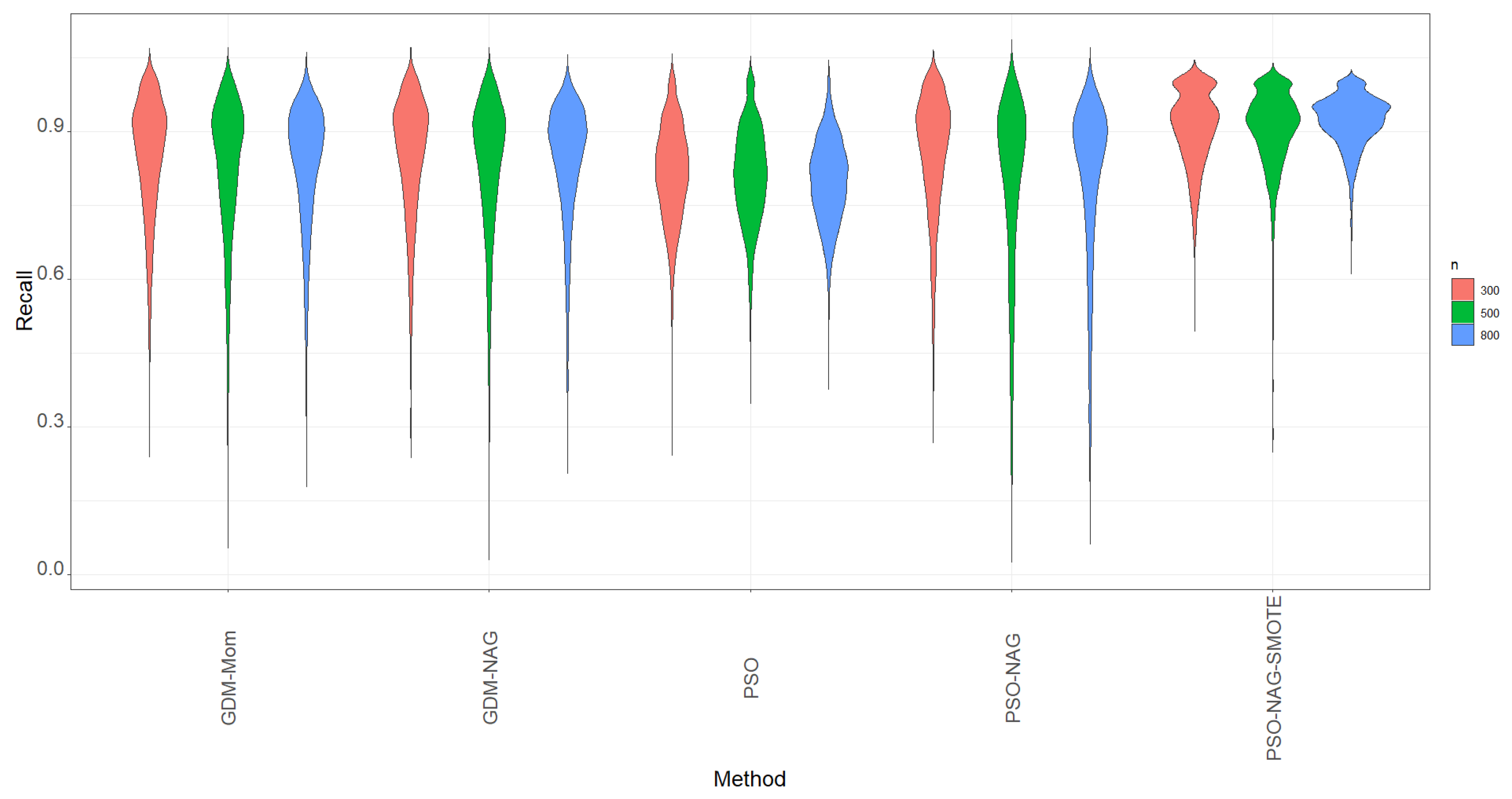
pso is used to implement the PSO algorithm. First, we focus on the metric of recall, which is the probability of correctly identifying if the positive case is truly positive. The violin plots of recall based on 1000 simulation runs for various methods are displayed in
Figure 1. The violin plots are a hybrid plots of the box plots and kernel density plots that are used to indicate summary statistics and the density of variables.
From
Figure 1, we can see that the GDM-Mom, GDM-NAG, and PSO-NAG methods have similar shapes and are competitive in terms of the recall metric. The PSO method can compute more quickly than all the GDMs. However, its performance in recall is slightly worse than the GDM-Mom, GDM-NAG, and PSO-NAG methods with a narrower spread range. To overcome the time-consuming drawback of gradient descent methods, we suggest obtaining the estimate of
based on the PSO method and then running the GDM-NAG method by replacing
with the mean of 100 PSO estimates of
. The method is named the PSO-NAG method. The PSO-NAG method can run more quickly than the GDM-NAG method.
In view of
Figure 1, we also find that data augmentation can help the ZIBer model to enhance the value of recall; that is, the ability of the ZIBer model to correctly identify if the positive case is truly positive can be enhanced after using the SMOTE method for data augmentation.
Figure 1 shows that the PSO-NAG-SMOTE method outperforms all the competitors in terms of a high value of recall and the narrowest spread range.
Figure 1.
The violins of recall based on 1000 simulation runs for various methods.
Figure 1.
The violins of recall based on 1000 simulation runs for various methods.
Recall is not the only metric to evaluate the ability to correctly identify the TP cases. We carefully study the ability to correctly identify the TP cases using the metrics of recall, precision, and their integrated metric, the
-score metric. All simulation results are reported in
Table 3,
Table 4 and
Table 5. As we have mentioned in the parameter settings, only
and
are used for the case of
for
Table 5 to allow the test sample to have more cases with
for model evaluation. Different from the screening process suggested by Xin et al. [
4], we use
-score instead of accuracy to determine the cut point. If we focus on the proportion of TP, high recall and precision mean that most TP cases have been successfully identified and most predicted positive cases are truly positive, respectively. A method with a high recall and precision is expected; otherwise, a balance between recall and precision is needed. Hence, the metric
-score is considered in this study to replace recall for assessing classification performance.
- 1.
The classification quality of the ENR-ZIBer model depends on the level of imbalance. The mean recall columns in
Table 3,
Table 4 and
Table 5 report high values, which indicates that the ENR-ZIBer model have a good ability to correctly identify the TP cases. However, we also find that the value of precision is significantly lower than the value of tecall.
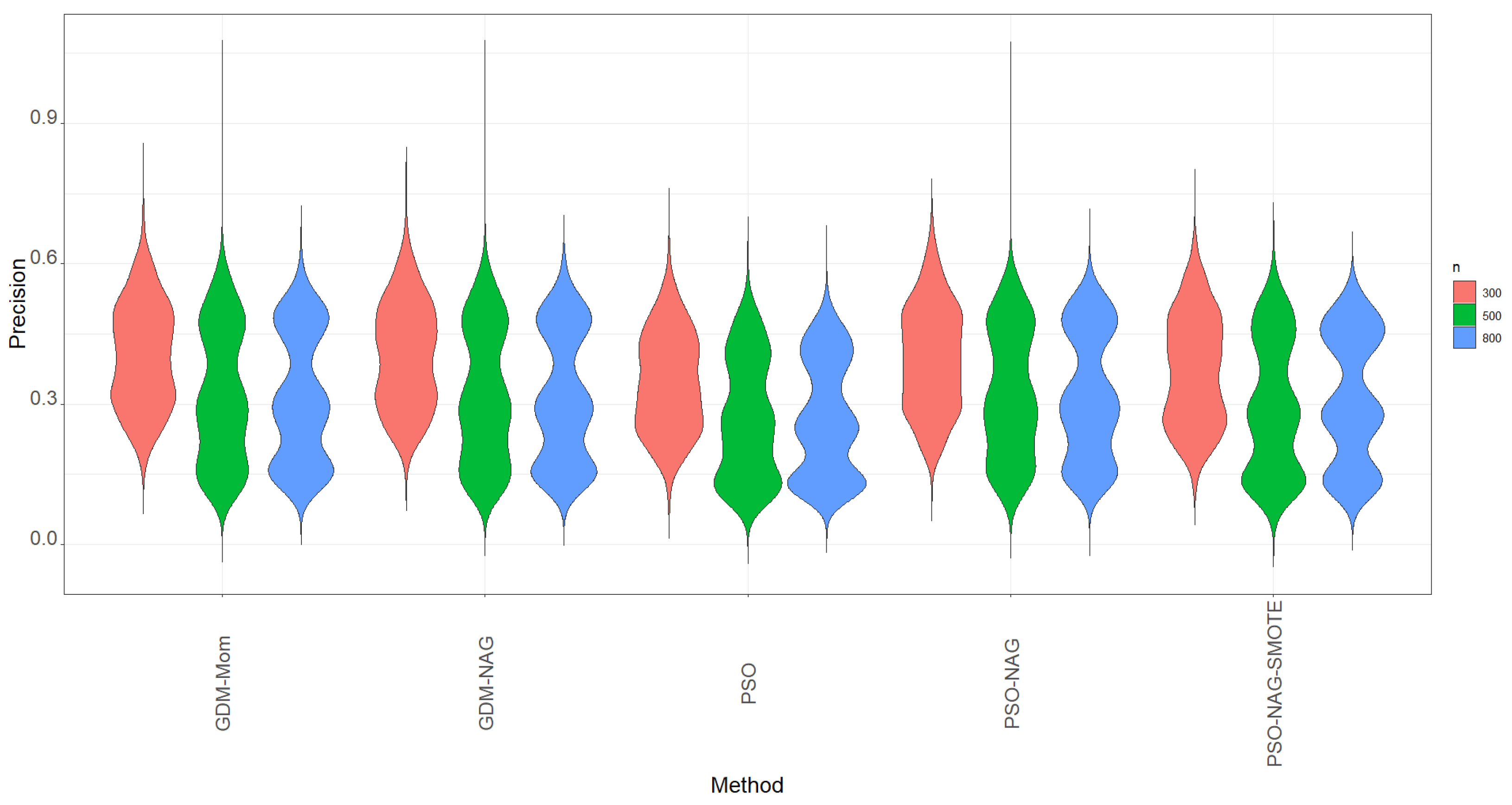
- 2.
The violin plots of precision based on 1000 simulation runs for various methods shown in
Figure 2 also indicate that the values of precision are lower than the values of recall shown in
Figure 1.
Figure 2 shows that the PSO-NAG method slightly outperforms the other competitors with a higher precision metric. The findings indicate that enhancing the ability to identify the TP cases through using the SMOTE method also incurs more FP cases in classification.
Table 5 shows that when the proportion of the minority group is lower than 10%, the precision significantly drops from the corresponding figures in
Table 3 and
Table 4. This is a trade-off to enhance the recall of the ENR-ZIBer model by using the SMOTE method for data augmentation.
- 3.
The rule of using a high
-score to screen out the best model hurts the accuracy. It is also important to have a compromise between correctly identifying the TP cases and keeping a high rate of TP prediction. Considering a higher value of the
-score as the metric to screen out the best model, we can find that the GDM-NAG algorithm outperforms the GDM-Mom and PSO algorithms for most of the cells in
Table 3,
Table 4 and
Table 5. Moreover, we can take advantage of the PSO algorithm, which can save computation time to obtain a reliable estimate of
. The PSO-NAG method is recommended due to the fact that it can save more computation time than the GDM-Mom and GDM-NAG methods.
- 4
Table 3,
Table 4 and
Table 5 show that the GDM-NAG method produces a similar estimation quality to that obtained by using the GDM-Mom method. The PSO algorithm works most efficiently to save computation time. However, its performance is inferior to the GDM-NAG and GDM-Mom methods. The PSO-NAG algorithm uses the PSO algorithm to obtain the estimate of
based on 100 iterations, and then to obtain the estimate of
using the GDM-NAG method and the PSO estimate of
.
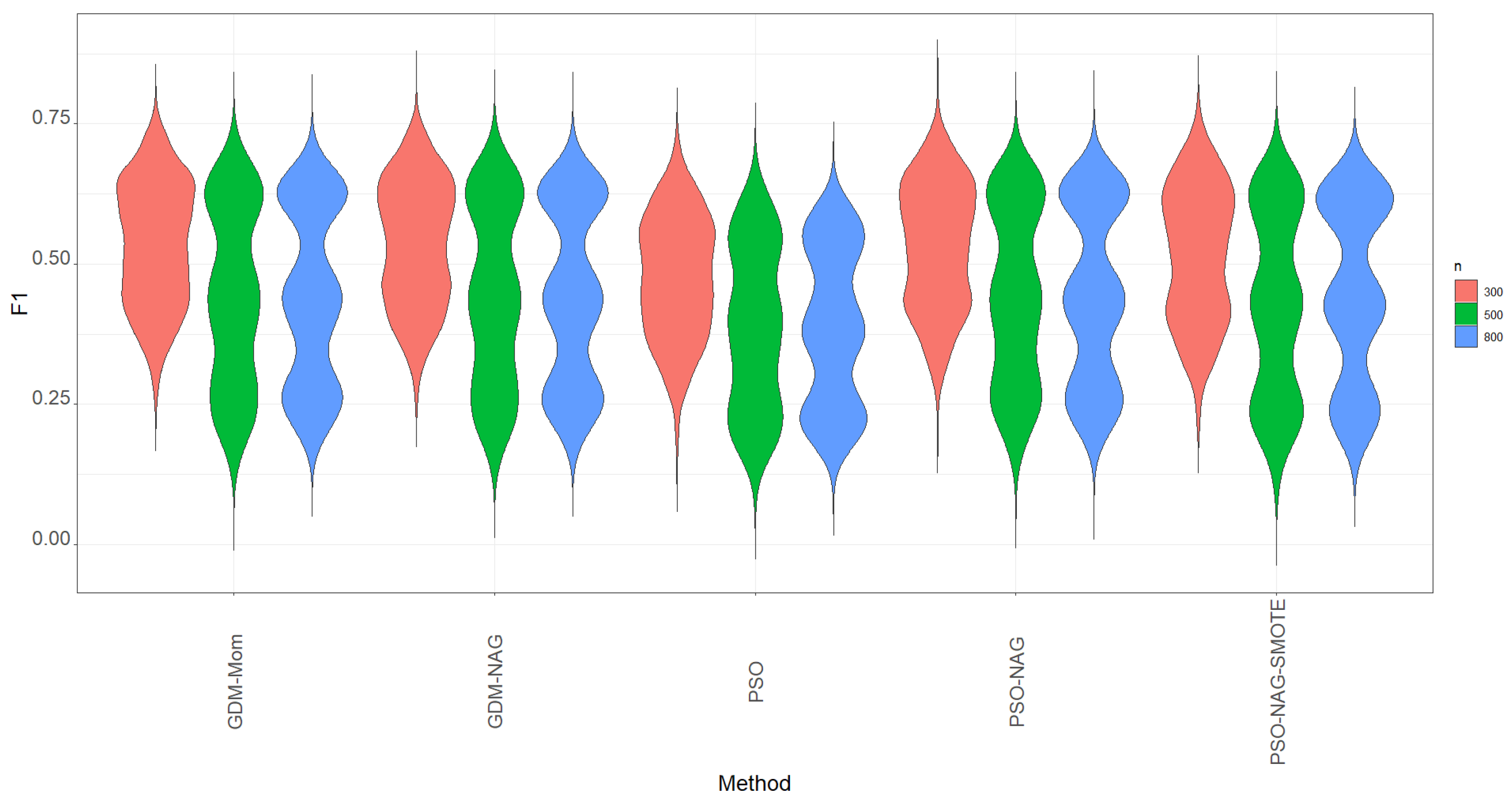
Table 3,
Table 4 and
Table 5 show that the PSO-NAG algorithm can be a good method to have a compromise between having a high
-score and saving computation time (
Figure 3).
- 5.
The SMOTE method significantly enhances the value of recall but also decreases the value of precision. After balancing using -score, we find that the proposed PSO-NAG method beats the PSO-NAG-SMOTE method. SMOTE is a popular technique to promote the performance of machine learning tools for imbalanced data. However, we find that the trade-off of using the SMOTE method for the ENR-ZIBer model is to enhance the value of recall but decrease the value of precision. Moreover, the PSO-NAG-SMOTE method consumes more computation time to work. The benefit of using SMOTE for the PSO-NAG algorithm in the ENR-ZIBer model is insignificant if the payoff for precision is considered. If dealing with FP cases is not an issue for practical applications, the PSO-NAG-SMOTE method is recommended.
- 6.
Table 3,
Table 4 and
Table 5 show that increasing the sample size helps to decrease the standard deviation of the metrics from the simulation study. Hence, reliable estimation results depend on the sample size. Basically, at least 300 observations in a sample are recommended to implement the ZIBer model if the level of zero-inflated data and imbalances is moderate. If the level of zero-inflated data and imbalances is extremely high, then at least 500 observations in a sample are recommended to implement the ZIBer model.
In summary, if dealing with FP cases is not an issue for practical applications, the PSO-NAG-SMOTE method is recommended. If we consider a balance between the metrics of recall and precision to implement the ENR-ZIBer model, the PSO-NAG method is recommended based on the -score. The recall value from PSO-NAG is significantly high overall in the simulation results. The findings indicate that the proposed hybrid algorithm with SMOTE for data augmentation can significantly enhance the ability to correctly identify the TP cases.
5. Concluding Remarks
In this study, we investigated the estimation quality of using the machine learning methods of PSO, GDM-Mom, GDM-NAG, PSO-NAG, and PSO-NAG-SMOTE to establish the ENR-ZIBer model when the dataset is zero-inflated or imbalanced. Monte Carlo simulations were conducted to verify the classification performance of the ENR-ZIBer model based on the holdout cross-validation method. The purpose is to find the best competitive machine learning method for the prediction of the ENR-ZIBer model and save computation time. The simulation results have shown that the hybrid algorithm, by integrating the PSO and GDM-NAG algorithms with two steps, is the most competitive in balancing the metrics of recall and precision.
The performance of the SMOTE method for data augmentation for the zero-inflated data was also studied in this manuscript. The PSO-NAG-SMOTE method enhances the ENR-ZIBer model’s ability to identify TP cases. However, the augmented data based on the SMOTE method also result in more FP cases in the prediction results using the ENR-ZIBer model. This is a trade-off in using the SMOTE method for the hybrid algorithm of PSO-NAG. In practical applications, the PSO-NAG-SMOTE method can be used to establish the ENR-ZIBer model if the issue of FP cases is not a concern. Only the PSO-NAD-SMOTE algorithm for simulations with 1000 iterations is time-consuming. In practical applications for small to moderate sample sizes, the computation time is acceptable.
Two datasets about Pima Indian diabetes and biopsy were used to illustrate the applications of the proposed method. In this example, the PSO, PSO-Mom, PSO-NAG, and PSO-NAG-SMOTE methods are used to establish the ENR-ZIBer model, and the performance is evaluated via utilizing the 5-fold cross-validation method. As we found in the simulation study, the hybrid algorithm outperforms the other competitors based on the -score metric. We also find the good ability of the ENR-ZIBer model to correctly predict the true positive cases.
Simulation results show that using the proposed PSO-NAG-SMOTE hybrid algorithms can enhance the recall of the ENR-ZIBer model. The findings indicate that the proposed hybrid algorithm with SMOTE for data augmentation can significantly enhance the ability to correctly identify the TP cases. How to reduce the possibility of FP cases in the prediction based on the data augmentation method is important. The ZIBer model uses a sigmoid function as a link function. It is easy to implement, but its performance has room to improve. The proposed method asks for using the median of 100 PSO estimates as the estimate of . It will spend more time on parameter estimation. To enhance the classification performance of the ENR-ZIBer model, how to combine the ENR-ZIBer model with other competitive machine learning methods is also interesting. These two topics are still open and will be studied in the future.


