Decision Support System to Solve Single-Container Loading Problem Considering Practical Constraints

Abstract

The container loading problem (CLP) has a broad spectrum of applications in industry and has been studied for over 60 years due to its high complexity. This paper addresses a realistic single-container loading scenario with practical constraints, including orientation limitations, maximum stacking weight, static stability, overall container weight limit, and fractional loading for multiple drop-off points (multidrop). We propose an open-source decision support system (DSS) implemented on a widely used platform (MS Excel®), which employs a heuristic algorithm to find efficient loading solutions under these constraints. The DSS uses a multi-start randomized constructive algorithm based on a maximal residual space representation. The constructive phase builds the loading pattern in vertical layers (columns or walls), while respecting all practical constraints. The performance of the proposed heuristic is validated through extensive computational experiments on classical benchmark instances, comparing its results against the recent state-of-the-art methods. We also analyze the impact of multi-drop constraints on utilization metrics. The DSS features an interactive interface for creating/loading instances, visualizing step-by-step packing patterns, and displaying key statistics, thus providing a user-friendly decision tool for practitioners.

1. Introduction

In 2020 and 2021, the COVID-19 pandemic posed great challenges for logistics operators worldwide due to the surge in online retail, home deliveries, and the global distribution of vaccines. Many companies in the logistics and delivery sector were pushed to their limits [1]. According to the Pitney Bowes Parcel Shipping Index (2022), global parcel volume in 2021 increased by 21% compared to the previous year, reaching 159 billion parcels—about 5000 parcels every second (or 436 million per day) [2]. This rapid growth is projected to continue, with annual parcel shipments possibly reaching 200–250 billion by the mid-2020s. Such trends underscore the importance of optimizing loading processes; efficiently utilizing container space and adhering to safe loading practices can help logistics providers handle more goods while controlling costs and maintaining service quality.

Within this context, the efficient loading of shipping containers (or truck trailers) has gained renewed attention. The three-dimensional container loading problem (CLP) involves packing a set of rectangular boxes into a container of fixed dimensions such that a given objective (typically maximizing volume utilization) is achieved without violating packing constraints. CLP is an NP-hard issue, and it becomes even more challenging when practical constraints are considered [3]. In real-world applications, boxes must not only fit geometrically but also satisfy constraints related to cargo orientation, stacking strength, stability, weight distribution, and delivery routes. Failing to consider these can lead to unsafe or impractical load plans. For example, boxes have limited allowed orientations (often only orthogonal rotations) and load-bearing limits (a box can support only a certain weight on top of it). The load must remain statically stable; each box should be supported by the container floor or other boxes underneath to prevent collapse. The total weight in the container cannot exceed its capacity, and the weight might need to be balanced to prevent axle overloads. Moreover, in multi-drop scenarios where a container carries orders for multiple destinations, the packing must be organized such that items for the first drop are accessible without unloading the items for later drops [4].

According to [5], the CLP is classified depending on the assortment of items to be placed. If the assortment is strongly heterogeneous, this problem is called the three-dimensional single-knapsack problem (3DSKP). If the assortment is highly homogeneous, this problem is classified as the three-dimensional single-large-object placement problem (3DSLOPP). In this work, the CLP—regardless of the assortment of items—is solved.

Commercial products, such as EasyCargo^®, CubeMaster^®, SIC [6], and Esko^®, among other software, offer a solution for efficiently planning cargo within a container or truck. However, the use of these products requires considerable monetary investment. This paper proposes an open-source and free access decision support system (DSS) as a Microsoft Excel^® spreadsheet with Visual Basic for Applications (VBA). This tool is expected to allow logistics operators from small- and medium-sized companies to better distribute their shipments and make their operations more efficient. Additionally, it will allow future researchers to compare their results and improve the proposed algorithms.

The proposed DSS solves the CLP regardless of the assortment of items (3DSKP and 3DSLOPP), considering the geometric containment constraints, item overlap, practical box constraints—such as the allowable orientation and static stability—maximum weight limitations related to box stacking and container, and loads to be delivered at different destinations (multi-drop).

Based on the motivations outlined above, this study is structured to resolve the following two primary research questions:

• RQ1: How can a decision support system (DSS) be designed to efficiently assist in packing problems with practical delivery constraints, ensuring both operational feasibility and high container space utilization?
• RQ2: How can the strict multi-drop constraint be relaxed through penalty mechanisms to balance container space optimization with practical unloading requirements, and how can this trade-off be made transparent to the end-user?

This paper is organized as follows: In Section 2, the CLP constraints are stated, and the multi-drop constraints and some smoothing variations of these constraints are explained. Section 3 explains the proposed solution methodology, and the steps of the implemented algorithm are also presented. In Section 4, the results are discussed, and comparisons with the previous work and smoothed models are described. Finally, Section 5 presents some conclusions and the recommendations for future research.

2. Problem Definition and Related Work

We consider a single rectangular container of fixed length L, width W, and height H. A set of n boxes (items) is given, where each box i has dimensions $({\mathcal{\ell }}_i,w_i,h_i)$, weight $p_i$, and belongs to a certain customer order (or destination) denoted by $d\left(i\right)\in \{1,2,\dots ,D\}$ if there are D distinct drop-off points. The objective is to pack a selection (ideally all) of these boxes into the container to maximize volume utilization (or equivalently, to minimize wasted space), subject to the following constraints:

No Overlapping (Geometry): Boxes must be placed axis-aligned (orthogonal packing), with their faces parallel to the container walls. No two boxes may overlap in space, and each box must lie entirely within the container boundaries.

Orientation Constraints: Each box may have a restricted set of allowed orientations. In our case, we allow the rotation of boxes such that their base lies on the container floor (i.e., no turning a box to rest on a side or its top, if that is deemed inappropriate). Following [7], this is implemented via binary parameters indicating which of the six face orientations are permitted for each box. Many practical applications disallow certain orientations due to labeling, handling, or stability (e.g., “this side up”). In our model, we assume that all boxes must be placed upright in one of the predefined allowed orientations.

Static Stability: According to [8], the objective of vertical stability is to guarantee that the boxes remain stationary during the container loading process. In this work, every box placed must have its entire base supported either by the container floor or by the top surface(s) of one or more boxes directly underneath it. We enforce the full support rule to guarantee vertical stability of the load; no box can hang partially in the air without support. This is stricter than some approaches (which allow a small overhang), but it ensures that boxes will not tip or tumble during loading. The trade-off is a possibly lower packing density, as some voids might be left to preserve stability.

Stacking Strength (Load-Bearing Constraint): Each box i has a maximum load capacity (often given in kg or N, sometimes as “crush resistance”). We interpret this as a constraint that limits the total weight of boxes stacked on top of box i, as proposed by [9]. For any box i, the sum of weights of all the boxes placed above it (i.e., those that directly or indirectly rely on i for support) cannot exceed $S_i$, the stacking strength of box i. In practice, $S_i$ might be provided by the box manufacturer (e.g., “do not stack more than 200 kg on this box”). We approximate the distribution of weight by assuming that if a box j sits on top of box i, it distributes its weight evenly on i’s top face. If box j overlaps multiple boxes beneath, its weight is split proportionally to the overlap area (as per the common assumption in load-bearing models). This way, we can accumulate the load on each box and ensure it does not exceed its capacity. Our heuristic checks this incrementally; whenever a new box is placed on top of others, we update the support load on those beneath and verify that none exceeds their limit. If a placement might violate a stacking constraint, it is disallowed.

Maximum Container Weight: The sum of the weights of all the boxes in the container must not exceed the container’s rated capacity (e.g., a 20 ft container might have a maximum payload of around 21,600 kg). This is a simple knapsack-type constraint, which can be expressed as follows: ${\sum }_{i\in \mathrm{packed}\text{-}\mathrm{items}}{p}_i\le P_{max}$. In practice, this limit is usually provided on the container’s safety plate. In our problem instances, we ensure not to load beyond this limit. The heuristic can easily track the total weight added and avoid selecting boxes that would cause an overflow.

Multi-drop (Delivery Sequence): According to [9], organizing boxes based on customer orders and their unloading priorities ensures efficient handling during the unloading process. Specifically, all boxes belonging to the same customer’s order must be grouped together without splitting across multiple sections of the container. Specifically, boxes from different orders should be organized so that, during unloading, workers handle only boxes from one customer at a time. In our approach, we assume that the D delivery destinations have a predefined unloading priority—given by $1\prec 2\prec \cdots \prec D$—typically established by a planned delivery route. To streamline the unloading process at each stop, we impose a constraint where all boxes for destination 1 must be placed closer to the container door than any box for destination 2, continuing sequentially through all subsequent destinations. We implement this by introducing up to $D-1$ virtual walls that partition the container loading space into D distinct segments. Each virtual wall is an imaginary vertical plane parallel to the container’s width, ensuring no box intended for a later destination is positioned closer to the door than a box designated for an earlier destination. The detailed interpretation and implementation of these virtual walls are further clarified in the following sections.

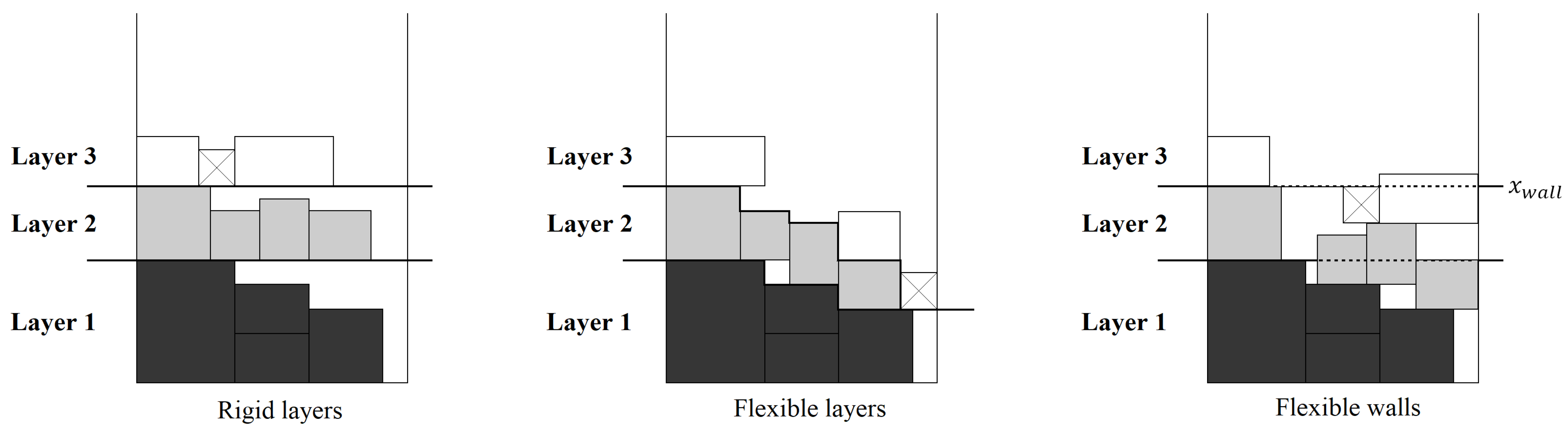
2.1. Multi-Drop Constraints

Load fractionation constraints are useful when a container must be packed with items destined for different customers. Ideally, items belonging to the same customer are packed closely together and positioned in the container so that the sequence of destinations in which they are unloaded is followed; thus, at each stop, it is not necessary to unload and reload the items [10].

According to [8], guaranteeing multi-drop constraints facilitates container unloading. Thus, all the items to be unloaded at a destination must be accessible without rearranging the other items. This condition is achieved by following the last-in, first-out (LIFO) principle. That is, if the destination of box i is visited before the destination of box j, item j must not be placed above item i or blocking the path from item i to the door. Thus, to avoid unnecessary operations, items with the same delivery location should be packed close to each other and placed in certain positions according to their destinations.

Furthermore, according to [11], cargo splitting is a combination of security (physical positioning) and logistics (customer positioning) constraints. The “physical positioning” constraint restricts the position of the boxes within a container. This constraint is generally dictated by a box’s size, weight, or content and requires that a specific item be placed—or not placed—in a particular position (for example, large items must be placed on the floor of a container). The constraint of “customer positioning” or grouping requires that a subset of items be loaded together or at a certain distance from each other to facilitate the loading and unloading processes, considering that some items, such as food and chemicals, should not be placed side by side.

Multi-drop deliveries can be applied in a restricted model to ensure the placement of all boxes belonging to the same customer before moving on to those of the next customer; it can also be applied in an unrestricted model, which does not impose the condition of packing all the boxes for a customer to continue with those of the next customer. In the three-dimensional loading of containers, the multi-drop approach is usually interpreted as concepts related to visibility, reachability, and separability.

Visible boxes: To facilitate efficient unloading, each box should have a clear path from its position to the container’s entrance. Upon reaching a specific delivery destination, each box to be delivered at this destination must be fully visible from the container’s door. Boxes belonging to the same destination can be arranged freely and may block each other. This concept has been effectively utilized by [12] within their tree-search heuristic. Ensuring compliance with this constraint means that boxes destined for later stops must be placed either behind or below those scheduled for earlier unloading. Geometrically, compliance is achieved when no box for a subsequent destination (j) is placed directly above a box designated for the current destination (i); specifically, the lower vertical coordinate ($z_1$) of box j must remain below the top vertical coordinate ($z_2$) of box i (see Figure 1). Additionally, boxes for later destinations must be placed behind the current destination’s boxes relative to the container door. In other words, the horizontal coordinate ($x_1$) of any subsequent destination box j must be behind the horizontal coordinate ($x_2$) of the current destination box i, ensuring unloading efficiency and accessibility at each stop. Several other studies have considered this definition [1,13,14,15,16,17,18,19,20,21,22,23,24].

Figure 1. Virtual wall application with $\delta =0$.

Reachable boxes: Although boxes are visible, they cannot always be easily reached by a person or a machine when unloading them. According to [25], a box is considered reachable if the distance between the box and the feet of the unloading operator is not greater than a defined constant. The reference point of the operator’s feet is measured from a point on the floor of the container that is closest to the reference box, where $L_{attainable}$ and $H_{attainable}$ represent the distance between an item and the operator’s feet on the x-axis and the z-axis, respectively. Equations (1) and (2) must be met for an item to be reachable. This constraint was also used in works such as [1,19].

$$L_{attainable}+H_{attainable}=200$$

(1)

$$L_{attainable}=min(200-z_i,60)$$

(2)

Boxes separated between customers/destinations: Ref. [26] introduced the parameter $\delta$ to control how much an operator is allowed to exceed the “border” between the boxes of consecutive destinations during unloading. This border is defined as a virtual wall, established after placing all the boxes belonging to a given destination inside the container. If $\delta =0$, a strict separation is enforced; the boxes for the next customer must be completely isolated from the previous customer’s boxes, and the operator is not allowed to cross the virtual wall to access them. In more flexible cases, when $\delta =l_i$ (where $l_i$ is a given length allowance), the operator may partially cross the border to reach the next group of boxes, allowing a small overlap between destinations. This constraint was also incorporated in the work of [19]. Figure 1 illustrates an example of virtual wall creation when $\delta =0$, where the blue boxes represent the items corresponding to the current destination or customer.

In this work, multi-drop is considered as a hard constraint, and our default implementation is the virtual walls, corresponding to the case where $\delta =0$, meaning that boxes for different destinations must be completely separated, and no overlap is allowed. Additionally, box relocation during unloading at the destination is prohibited. Although strict separation and the prohibition of relocation enhance unloading efficiency, they reduce the flexibility of the optimization process, which can negatively affect both the container space utilization and the overall operational performance.

The box relocation is not allowed at the destination or customer delivery time. This situation can result in an inflexible model that affects the algorithm’s efficiency and the actual operation. In cases where a delivery is made to a facility without sufficient space, item relocation may be unacceptable. However, relocation can be considered in cases where allowable by the delivery facility; therefore, relaxing this constraint could increase the volume of boxes. This aspect implies a balance between the volume of boxes and the indirect costs incurred when relocating items in the delivery. As proposed by [1], a way to soften the multi-drop constraints is to modify the objective function so that instead of maximizing the volume of boxes, it is possible to maximize the volume of boxes minus a series of penalties ($P_A,P_V,$ and $P_R$) when one of the boxes already placed violates any of the multi-drop constraints defined as follows:

Boxes above: The boxes that will be unloaded at the destination i can only have other boxes going to the same destination on their surface.

Visible boxes: The boxes that will be unloaded at the destination i must be completely visible from the container door.

Reachable boxes: The boxes to be unloaded at a destination must be reachable by a human operator, machine, or forklift.

A penalty is calculated depending on the constraint when any constraints are violated. For this case, we use the linear functions proposed by [1], as shown in Equations (3)–(5). Here, item i is the item to be downloaded. A check is performed to determine if item j violates any of the constraints; $z_j$ is the coordinate $z_1$ for the item j; $d_{ij}$ is the distance between items i and j; $w_j$ represents the weight of the item; and $v_j$ represents the volume of the item. The parameters $\gamma ,\alpha ,$ and $\beta$ need to be tuned.

$$P_A=(1+\gamma z_j)·(\alpha w_j+\beta v_j)$$

(3)

$$P_V=(1+\gamma z_j)·(\alpha w_j+\beta v_j)$$

(4)

$$P_R=(1+\gamma d_{ij})·(\alpha w_j+\beta v_j)$$

(5)

2.2. Related Work

Recent studies on the CLP reflect a strong emphasis on practical constraints and on solution methods that can handle real-size instances. On the one hand, there has been progress in the exact methods for solving the CLP, with researchers formulating comprehensive mixed-integer programming models to capture real-world requirements [27]. On the other hand, due to the inherent NP hardness and large instance sizes in the industry, many heuristic and metaheuristic methods have been developed to produce high-quality solutions within feasible computation times. In parallel, learning-based approaches have attempted to tackle dynamic versions of the problem and scenarios involving uncertainty [11,28,29]. We review both categories, focusing on key constraints such as orientation, stacking (load-bearing limits), static stability, multi-drop (loading/unloading sequence), and weight limits.

Traditional exact algorithms for CLP (e.g., branch-and-bound or branch-and-cut formulations) could solve only small instances or simplified variants. In the past ten years, researchers have significantly improved exact formulations to handle more complex constraint sets. For example, Ref. [24] presented an integer linear programming model that integrated a comprehensive set of practical constraints (including orientation, full support stability, stacking strength, and weight limits). They developed an exact algorithm based on arc-flow formulations and decomposition, capable of finding optimal solutions for moderate-sized instances of the single-container loading problem. Similarly, Ref. [30] proposed an exact method for addressing several types of container loading problems (with different constraint combinations); their approach systematically enumerated feasible packing options and was tested on multiple benchmark variants. These works demonstrate that it is possible to model the CLP with realistic constraints in an exact optimization framework. However, the solvable instance sizes remain limited. Even with these advanced models, the computational effort grows exponentially with the number of boxes. As noted in a recent study, state-of-the-art exact algorithms can handle the order of only a few hundred items at best (for instance, considering stability constraints, around 180 items was a practical limit in some studies) [31]. This is far from the thousands of items that might appear in real logistics operations. Indeed, exact methods are still often too slow for large-scale, time-sensitive applications, especially when multiple constraints restrict the packing arrangements.

To overcome some of these limitations, researchers have also explored matheuristics (hybrid methods combining exact and heuristic components). Ref. [32] developed a matheuristic framework for a single-container loading problem with practical constraints. Their approach used an integer programming core to place large “key” items or layers, and heuristics to fill the remaining spaces, effectively balancing optimality and speed. This approach was shown to find optimal or near-optimal solutions faster than a pure ILP solution for many cases. Another notable contribution was by [33], who introduced a new 3D packing model (with unified assignment and packing variables) to better handle box rotation and positioning constraints in a single MILP formulation. While such formulations are elegant, they can become very large and were primarily tested on small instances due to computational limits.

In terms of specific constraints, one area of interest is static stability. Classical models often enforce stability by requiring that each box is fully supported by others beneath it (no unsupported overhang). This “full support” constraint guarantees that no box will tip or fall. However, it can be overly restrictive, sometimes leaving container space underutilized. Recent exact approaches have introduced more nuanced stability criteria. For instance, Ref. [34] investigated cargo stability through support factors and mechanical equilibrium conditions. Instead of demanding 100% base support for every box, they allow partial support as long as stability metrics (like the center of gravity projection or a minimum support area ratio) are satisfied. In the same vein, Ref. [35] proposed a static equilibrium-based check for stability, integrating it into a branch-and-cut algorithm. By treating each packed box as a rigid body and ensuring the net torque due to gravity is balanced (no tipping point), they can accept packing solutions with partial overlaps that are still stable. Their results showed improved container utilization compared to the traditional full-support rule, without compromising safety. These developments highlight that exact methods are evolving not just to handle more boxes but also to incorporate more realistic physics of stacking and stability. Nonetheless, even with these improvements, exact solvers typically struggle with large-scale instances or tight time limits, which is why heuristic approaches remain indispensable for practical use.

Given the computational complexity of CLP, heuristics have long been the workhorse for practitioners. The past five years have seen advanced heuristics that can accommodate complex constraints while still producing solutions quickly. A common strategy is to build packings iteratively (greedily or with randomization) and use local search or other metaheuristic frameworks to improve upon an initial solution. Many recent algorithms leverage the concept of maximal spaces (also known as empty space or residual space representation) to decide where to place the next box or sub-stack. This concept, originally popularized by algorithms in the 2000s, fits well with constraint handling, as each placement simply reduces the available free space which can then be evaluated for further placements. Modern heuristics often combine this with Greedy Randomized Adaptive Search Procedures (GRASP) or Large Neighborhood Search (LNS) to explore a variety of packing patterns.

For example, a recent work by [4] embedded a mechanical stability model into a reactive GRASP algorithm. In their approach, each iteration constructed a packing plan by selecting feasible box placements (often grouping boxes into “blocks” or layers) and used a randomized greedy criterion to pick the next placement. After a complete packing plan was constructed, they evaluated its dynamic stability using a physics-inspired model (simulating the effect of tilting or movement) and discarded or penalized unstable solutions [36,37]. This hybrid approach ensured that every solution generated not only used space efficiently but also met the stability, orientation, weight, and multi-drop constraints by design. Their algorithm was tested on scenarios with multiple drop-offs and showed that incorporating stability checks during the search leads to more robust load plans, albeit sometimes at a slight cost in volume utilization.

Another state-of-the-art heuristic is the randomized constructive algorithm with multi-criteria sorting proposed by [3]. They tackled a real-world CLP variant with an exceptionally rich set of constraints, including the following: customer-specific unloading priorities (a strict form of multi-drop where the sequence is predetermined), load balancing within the container, cargo stability and stacking constraints, and even the minimization of unnecessary rearrangements during deliveries. Their method built the packing plan by first combining items into larger composite “blocks” in a preprocessing step and then sorting these by multiple criteria (value density, fragility, etc.). A randomized tie-breaking mechanism was used so that multiple packing orders could be explored. The boxes were then placed one by one (or block by block) respecting all constraints; if an item might violate stability or stacking limits, it would be skipped and possibly packed later. They also introduced soft constraints for the unloading sequence; if needed, a box for a later customer could be placed in front of one for an earlier customer but a penalty is incurred, reflecting the extra unloading effort. This enabled a trade-off between the perfect drop-off order and space utilization. In large-scale industry instances (hundreds of boxes, many different sizes), their heuristic found near-optimal solutions in seconds and even outperformed the company’s existing manual solutions and a commercial packing software. Notably, [3] reported that their algorithm was deployed in a real logistics firm, yielding significant economic benefits and CO₂ savings. This exemplifies the level of practicality and efficiency that modern heuristics can achieve.

Local search and neighborhood-based techniques also feature prominently in the recent research. Ref. [38] developed a Large Neighbourhood Search (LNS) algorithm for the single-container CLP, which iteratively destroys part of a packing solution and reoptimizes it, to escape the local optima. Their method returned results comparable to or better than those of the previous state-of-the-art heuristics on benchmark sets. The strength of LNS is its ability to make large-scale rearrangements (e.g., unloading and re-loading a subset of boxes differently) in each iteration, which can overcome the myopic decisions made in an initial greedy packing. By carefully designing the removal and reinsertion heuristics to respect constraints, the LNS can effectively navigate the solution space even for heavily constrained problems. For instance, the LNS might temporarily remove a few layers of boxes and attempt to re-pack them in a different order (still obeying stacking and stability rules) to improve overall volume usage or to better accommodate a multi-drop sequence. Such advanced local search frameworks benefit from today’s increased computing power, allowing many iterations and evaluations within a short time.

Multi-drop constraints have received special attention in the recent literature. In the classical CLP, all boxes are considered equivalent aside from size and maybe weight, but in multi-drop scenarios, boxes are grouped by customer or destination and a loading order constraint is imposed. Recent approaches have attempted to soften this, including the following: Ref. [1] formulated a multi-drop loading problem with soft unloading constraints. This MILP model, solved with a standard solver, could optimally pack moderate-sized instances and quantify the trade-off between packing efficiency and unloading effort. On the heuristic side, Ref. [39] addressed a multi-drop problem that also included split delivery conditions (where a single customer’s order might be split across multiple containers). They considered a fleet of containers for loading and aimed to meet all the customers’ demands with as few containers as possible, following a given delivery route. The authors proposed a multi-stage heuristic; first, pallets were assigned to containers (an allocation phase) and then a packing heuristic was applied to each container, ensuring that the boxes within each container were ordered by drop-off point. Their algorithm effectively integrated routing decisions (which drop is assigned to which container) with packing, yielding high utilization and honoring delivery constraints in computational tests.

3. Proposed Methodology

Given the complexity of the problem, we design a heuristic that builds solutions incrementally and uses randomization to explore different packing solutions. The core of our approach is a Multi-Start Randomized Constructive Algorithm (MSRCA). Each iteration of MSRCA attempts to pack the container from scratch, and after many iterations, we keep the best solution found. Because the heuristic is relatively fast per iteration, we can afford a large number of restarts, which improves the chances of finding a high-quality packing solution (in terms of volume usage) that also satisfies all constraints and can be easily embedded in a decision support system coded in Visual Basic for Applications (VBA).

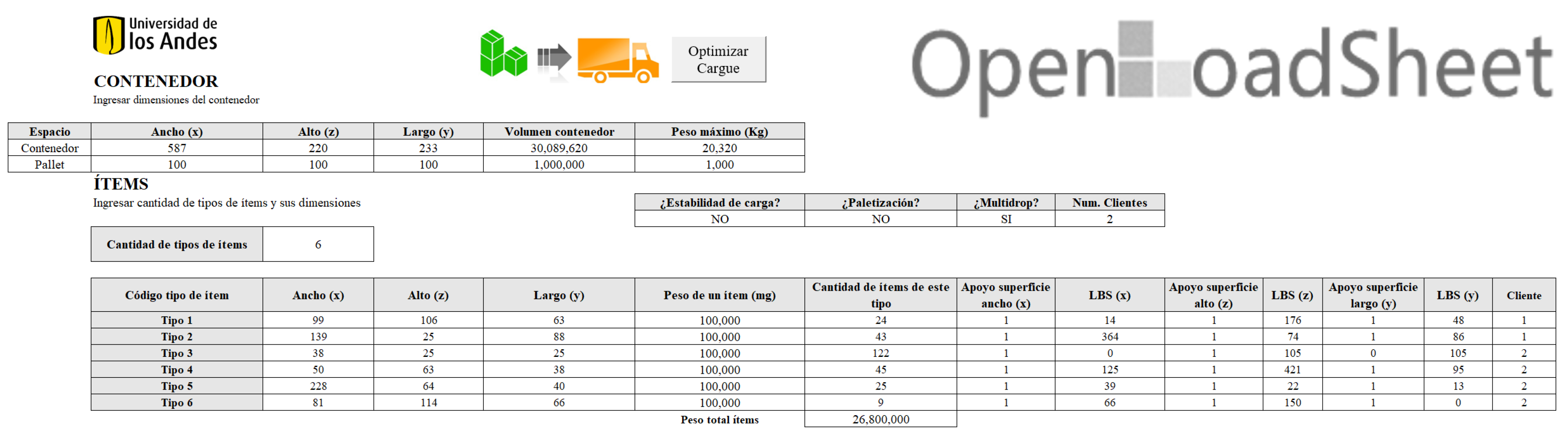
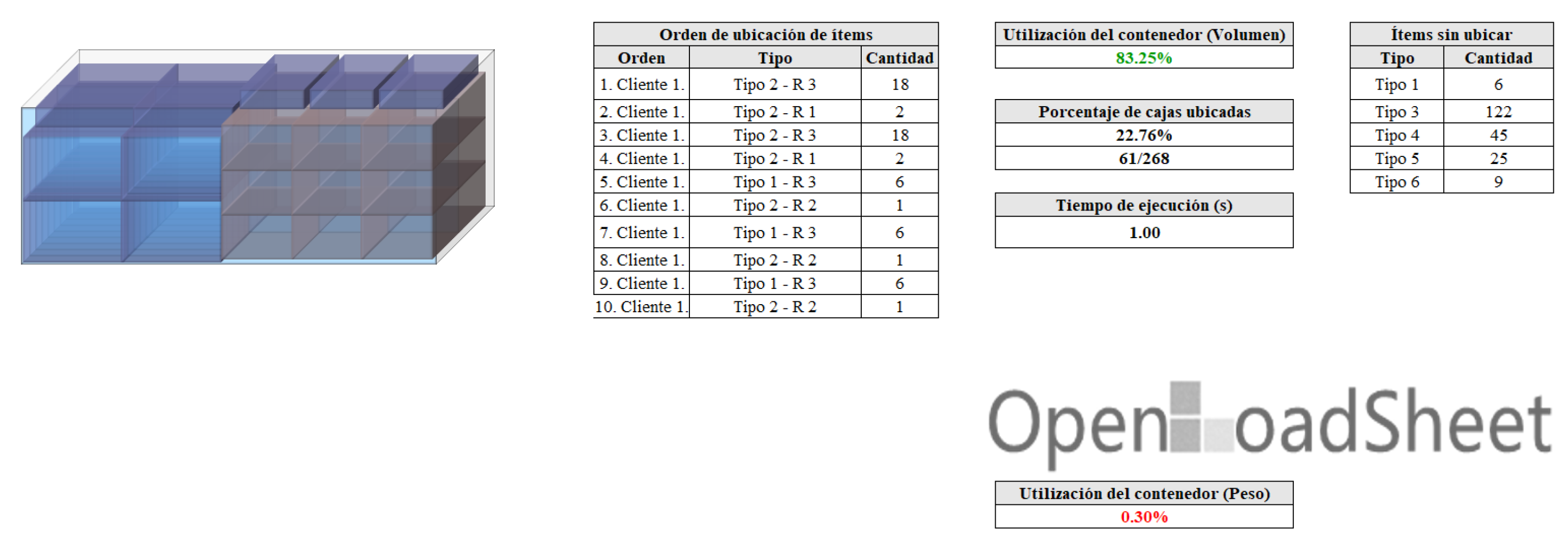
3.1. Decision Support System (DSS)

The proposed DSS incorporates static stability, six allowed orthogonal orientations, stacking limits, container weight limits, and multi-drop constraints (virtual walls, where $\delta =0$). To enable those functionalities, the user must enter the information related with the items. Once all the information is available, the optimization algorithm carries out an iterative process of randomized construction. In each iteration, the algorithm considers all customers and their items/sets of boxes, an iteration will be terminated if no spaces are available in the container. The algorithm will terminate early if all the boxes are successfully loaded, regardless of the iteration.

Figure 2 shows the home screen of the DSS, in which the parameters relevant to the container, boxes, and customers are entered. In Figure 3, the results are visualized. This figure shows relevant indicators, such as the percentage of the volume occupied, container weight, number of boxes placed, the order and rotation of these boxes, and the corresponding customer information.

Figure 2. Home screen with input of container and box parameters.

Figure 3. Results screen, relevant indicators, and location of boxes.

3.2. Optimization Algorithm

The proposed heuristic uses the representation of maximum residual spaces—MSRCA. Each time a box is placed, six maximum spaces are created. In addition, the boxes are placed as layers of boxes; if there is more than one box with the same dimensions and characteristics, a column or wall is created, combining the Y- and Z-axes.

Figure 4 shows an example of the layer construction when attempting to position ten identical boxes. The aim is to place as many boxes as possible along the first axis. Once the first row of boxes has been placed, the same row is repeatedly moved along the second axis, always maintaining the rectangular shape. This algorithm terminates when either all the boxes are positioned or there is no more space inside the container.

Figure 4. Combinations of axes for the formation of layers of boxes.

The MSRCA consists of the following five main steps:

Step 0: Initialization

The $BoxList$ is a list with all the boxes entered by the user, representing the boxes that should be placed in the container. Each time a box is placed, it is removed from the list, thereby maintaining an updated list. The $CustomerBoxList$ is a new list associated with the items that belong exclusively to each customer. The $LocationList$ is an updated list with all the boxes in the container. The list is initially empty and subsequently updated as the boxes are placed. The $SpaceList$ is an updated list with all the spaces available in the container. This list is initialized as a single-container-sized space and is updated each time a box or layer of boxes is placed.

Step 1: Space Selection

One of the spaces in the $SpaceList$ must be selected to place a box. The most suitable space is the one farthest from the entrance of the container. The space with the smallest coordinate on the X-axis is chosen in our case. In the event of a tie, the space with the smallest coordinate on the X-axis and the largest coordinate on the Z-axis is chosen, and the aim is always to stack boxes, or layers of boxes, as effectively as possible.

Step 2: Box Selection

Once a space S is chosen in Step 1, each remaining box belonging to the current customer (from the $CustomerBoxList$) must be evaluated for possible placement. When more than one box has the same dimensions, a layer of boxes must be created as a column or a wall. Two criteria are considered to choose the best box or layer of boxes to be placed in the maximum space previously chosen. The first would be a larger volume, as we seek to place the box or layer of boxes that occupy a larger volume in the space S; for all rotations, the volume will be the same. The second consideration would be best fit; we seek to place the box or layer of boxes with the best fit within the maximum space S, that is, the layer of boxes with the smallest combined distance between the sides of the layer and the sides of the space where it is to be positioned. In this case, the fit is calculated for each rotation of the box.

For the formation of the layers, the maximum load force constraints implemented by [40] are also considered because not all box configurations are feasible given this constraint. Furthermore, since the algorithm seeks to guarantee a restricted multi-drop model, it will never be possible to create layers of identical boxes that belong to different customers.

Once the box or box layer is placed, it is removed from the $BoxList$ and the $CustomerBoxList$, and added to the $LocationList$.

Step 3: Space List Update for Current Customer

Every time a box or layer of boxes is placed in a space S, the spaces in the $SpaceList$ intersected by this box or layer will be removed, and a maximum of six new spaces will be produced. However, not all of these new spaces will be feasible with the constraints of this problem. Once the six new spaces are created, each one is evaluated under the problem’s constraints, and only those that comply with the constraints will be added to the $SpaceList$. The spaces created must comply with the following constraints: (1) The volume available in the space must be sufficient to place at least one of the current customer’s boxes in any of its orientations. (2) The maximum load force constraints are met for the boxes on the floor of the new space. In this way, in the $SpaceList$, only the feasible spaces will be added based on these constraints, and those that are not feasible are excluded from the list. If boxes from the same customer still need to be placed, we return to Step 1. If all the boxes for the current customer have been placed, we proceed to Step 4. The algorithm terminates if the $SpaceList$ is empty or there are no more boxes to place.

Step 4: Space List Update for Next Customer

Once all the boxes for a customer/destination are placed in the container, the $SpaceList$ is updated before placing the boxes for the next customer/destination. A virtual wall ($x_{wall}$) separating different customer boxes will be generated from the point of the maximum value of $x_2$, i.e., the corner of the box that is closest to the door when the customer is changed. Next, the entire $SpaceList$ is evaluated, and all the existing spaces that have a coordinate $x_2$ are eliminated if they are not greater than or equal to $x_{wall}$.

For any remaining spaces where $x_1<x_{wall}$, the space must be modified to respect the newly created virtual wall. Specifically, the space is truncated by shifting its lower boundary along the X-axis; the original $x_1$ coordinate is updated and set equal to $x_{wall}$. This adjustment ensures that the usable portion of the space lies entirely in front of the virtual wall, preventing any future placement of boxes in the areas reserved for the previous customers. The algorithm iteration is terminated if the $SpaceList$ is empty upon removing the spaces.

Randomness

Each time a space S is selected, the box or layer of boxes to be placed within it is determined using one of the two previously described criteria. The choice between these two criteria is made randomly, with each criterion having an equal probability of being selected (50%).

After selecting one criterion, an attempt is made to identify the “best” box (or layer of boxes) according to the chosen criterion. To achieve this, an ordered candidate list $Candidates$ is created based on the indicator values for each box (or layer). Subsequently, a selection probability for each candidate is assigned according to its ranking/quality, following the harmonic series-based formula (see Equation (6)). Finally, one candidate is randomly selected based on the following probability distribution (${\rho }_i)$:

$${\rho }_i=1/(i·\sum _{j\in Candidates}1/j),\forall i\in Candidates$$

(6)

The optimization algorithm generates as output a packing pattern, which consists of a list of coordinates and orientations for each placed box. This packing pattern serves as the basis for visualization within the decision support system (DSS), where users can inspect the final layout or view a step-by-step animation of the loading sequence. Through this animation, users can observe the order in which boxes were placed and how container sections were progressively allocated to each delivery destination, providing valuable insights into the overall loading plan. Such transparency is crucial for fostering user trust in the DSS, as planners can easily verify, for instance, that all boxes corresponding to a given customer are positioned correctly and remain accessible.

The detailed procedure followed by the optimization algorithm is summarized in Algorithm 1, which outlines the multi-start randomized constructive method used to generate feasible packing solutions under practical constraints.

Algorithm 1 Multi-start randomized constructive algorithm for container loading.

Inputs: $BoxList$: List of boxes of each customer, $ReverseOrder$: List of costumers in reverse delivery order, $Dimensions$: Original container dimensions; Parameters: $TotalTime$: CPU time limit; Output: $Incumbent$: Best packing pattern.    1: $Incumbent\leftarrow \varnothing$    2: while $TotalTime$ is not consumed do    3:     $LocationList\leftarrow \varnothing$    4:     $SpaceList\leftarrow$ CreateEmptySpace($Dimensions$)    5:     for each customer $c\in ReverseOrder$ do    6:         $CustomerBoxList\leftarrow BoxList\left[c\right]$    7:         while $CustomerBoxList\ne \varnothing$ and $SpaceList\ne \varnothing$ do    8:            S← SelectEmptySpace($SpaceList$)    9:            if Rand() > 0.5 then  10:                $Layer$← SelectLayerRandomlyBestFit($S,CustomerBoxList$)  11:            else  12:                $Layer$← SelectLayerRandomlyMaxVolume($S,CustomerBoxList$)  13:            end if  14:            $LocationList$← Pack($Layer$, S, $LocationList$)  15:            $SpaceList$← UpdateEmptySpaces($Layer$, $SpaceList$)  16:            $CustomerBoxList\left[c\right]$← RemoveBoxes($Layer$, $CustomerBoxList$)  17:         end while  18:         $x_{\mathrm{wall}}\leftarrow$ CreateVirtualWall($PackedBoxes,c$)  19:         for each space $S\in SpaceList$ do  20:            if $S.x_2$$<x_{\mathrm{wall}}$ then  21:                $SpaceList\leftarrow$ RemoveSpace($S,SpaceList$)  22:            else if $S.x_1$$<x_{\mathrm{wall}}$ then  23:                $S.x_1\leftarrow x_{\mathrm{wall}}$  24:            end if  25:         end for  26:     end for  27:     if $LocationList.volume>Incumbent.volume$ then  28:         $Incumbent\leftarrow LocationList$  29:     end if  30: end while  31: return  $Incumbent$

3.3. Complexity Analysis of Multi-Start Randomized Constructive Algorithm

The algorithm constructs multiple packing solutions within a time limit parameter $TotalTime$. We denote n as the total number of boxes across all the customers and m as the number of destinations (customers). Each complete packing construction involves the following key steps:

• Initialization: Initializing the set of packed boxes and creating the initial empty space representing the container are considered constant-time operations ($O\left(1\right)$).
• Loop over customers: The algorithm processes each customer sequentially, implying $O\left(m\right)$ iterations at this level.
• Loop over boxes and spaces: For each customer, the algorithm iterates while there are remaining boxes and available spaces.
  • Selecting a space: Scanning or selecting a feasible space requires $O\left(\right|SpaceList\left|\right)$ time, where $\left|SpaceList\right|$ is the number of current empty spaces.
  • Layer selection: Building and randomly selecting a packing layer may involve checking all remaining boxes of the customer, costing $O(nlogn)$ operations.
  • Packing and updating spaces: Each packing operation removes a space and may create up to three new spaces. Hence, the number of spaces grows linearly with the number of boxes, leading to $\left|SpaceList\right|=O\left(n\right)$ in the worst case.
  • Updating box lists: Removing packed boxes is $O\left(1\right)$ per box.
  Consequently, each box incurs a cost of $O\left(\right|SpaceList|+nlogn)=O(nlogn)$, and processing all n boxes gives a total cost of $O(n^{2}logn)$ for this stage.
• Virtual wall insertion and space adjustment: After finishing the packing for each customer, the algorithm updates the $SpaceList$ list by checking each available space. As there are $O\left(n\right)$ spaces at most, and this check happens m times (once per customer), this step has a total cost of $O\left(mn\right)$.
• Best incumbent update: Comparing volumes and updating the incumbent solution is considered a constant-time operation ($O\left(1\right)$ per construction).

Summing the costs, a single construction has a total time complexity of $O(n^{2}logn+mn)$. Since $n^{2}logn$ dominates $mn$ when $n\gg m$ (which is usually the case in practical applications), the complexity simplifies to $O(n^{2}logn)$. The entire algorithm runs multiple constructions within the $TotalTime$ limit. Let k denote the number of completed constructions within the available time. Then, the global complexity becomes $O(k·n^{2}logn)$, where k depends on the computational time allowed and the average time per construction.

The primary data structures maintained are the list of packed boxes and the list of empty spaces. Both are bound by $O\left(n\right)$ elements, resulting in an overall space complexity of $O\left(n\right)$. Thus, the algorithm exhibits a time complexity of $O(k·n^{2}logn)$ and a space complexity of $O\left(n\right)$, where n is the total number of boxes and k is the number of construction attempts allowed by the CPU time limit.

It is important to note that our heuristic does not guarantee optimality. There may be some free space left even if not strictly necessary, due to the heuristic nature of the choices made. However, by comparing against known optimal or best-known solutions from the literature on standard instances, we ensure that the performance loss (if any) is small. The next section provides this comparison, along with an analysis of how the algorithm performs under different multi-drop settings. We also discuss computational efficiency; in our tests, the algorithm consistently runs within the set time limit (30 s) even for large instances with hundreds of boxes, thanks to the simplicity of each iteration’s operations and the pruning effect of constraints (fewer feasible placements means fewer candidates to evaluate in each step).

4. Computational Experiments and Analysis of Results

The performance of the proposed approach is validated by comparing it with leading algorithms found in the specialized literature. Specifically, computational effectiveness and efficiency are evaluated against prominent methods developed by [19,26,41]. The heuristic were coded in VBA. The computational experiments were conducted on a system equipped with an AMD Ryzen 5 4500U processor with Radeon Graphics (2.38 GHz, 8 GB RAM) using Microsoft Excel 2019^® software (v16.0).

The only parameter required by the proposed heuristic is the computational time limit ($TotalTime$), which in this work was set to 30 s per instance. This choice aimed to achieve low waiting-time responses, thereby ensuring an efficient and user-friendly experience within the decision support system.

4.1. Comparison with [19,26]

First, we compare our heuristic with the exact algorithm proposed by [26] and the GRASP algorithm presented by [19], which separates boxes for each customer by creating virtual walls. For this purpose, we use the set of instances presented by [26], which consists of 11 test cases with a number of pieces ranging from 20 to 1 thousand, a number of piece types varying between 1 and 20, two different container lengths (12 and 15 units), and a fixed number of three customers for all cases. The results reported by [26] correspond to the best integer solution (MIPSol) obtained by the solver within a one-hour execution time limit; meanwhile, the results published by [19] correspond to the incumbent subsequently obtained after 50,000 iterations. Comparing our heuristic with an exact method allows us to effectively evaluate the quality of the obtained solutions. Regarding the constraints considered, the exact algorithm presented by [26] is an unrestricted model that permits multiple drops; in other words, it does not enforce the condition of fully packing all boxes for one customer before proceeding to the next customer’s boxes. In the tested instances, ref. [26] aimed to maximize container volume utilization, although the results were reported in terms of the percentage of boxes packed, given that the evaluated scenarios represent perfect packing instances with known optimal solutions. Therefore, achieving 100% utilization both in volume and in the number of packed boxes was expected.

Table 1 shows the results obtained for the MILP of [26], the GRASP of [19], the MSRCA proposed, and the MSRCA without full support. As seen in this table, in the different instances, the proposed algorithm (MSRCA) either succeeds in placing 100% of the boxes in the container or improves the metric obtained by the exact implementation of [26] or the GRASP of [19]. It should be noted that the first instance A1 shows that the comparison made is not fair. In the publication by [26], it was mentioned that the formulation of the problem included a constraint that guaranteed the vertical stability of the load in a generalized way; however, this model could yield unstable solutions. In our work, the lower surface area of a box must be entirely supported by the upper surface of one or more boxes placed immediately below it or by the floor of the container (full support), always guaranteeing vertical stability.

Table 1. Comparison with [19,26].

Id	Container Length	Type of Boxes	Number of Boxes	Percentage of Located Boxes (%)
				MILP [26]	GRASP [19]	MSRCA	MSRCA Without FS
A1	15	1	20	100	100	100	100
	12	1	20	95	95	80	95
A5	15	5	41	100	100	100	100
	12	5	41	77.9	96	97.6	97.6
A10	15	10	99	100	100	100	100
A20	15	20	89	100	100	100	100
	12	20	89	92.8	98.4	96.6	96.6
B1	15	1	500	100	100	100	100
B5	15	5	813	100	100	100	100
B10	15	10	1000	100	100	100	100
B20	15	20	674	100	100	100	100
Average				96.88	99.04	97.65	99.02

For instance, in case A1, using a container length of $L=12$ units along the X-axis, the first virtual wall (${L_1^{\prime }}^{*}$) is placed at $x_{wall}=2$, as presented in Table 2 by [26]. This implies that the four boxes belonging to Customer 1 occupy only two units of length, a scenario achievable exclusively by allowing overhang. However, repeated overhangs cannot ensure vertical stability, this concept is illustrated graphically in Figure 5. Figure 5 demonstrates that a blue box placed atop a red box will remain stable, provided that less than 50% of its base is overhanging. Nevertheless, typical overhang models often do not validate stability for second-level placements. For instance, if a green box is placed on top of the blue box, both will collapse due to their center of gravity extending beyond the stable limits.

Table 2. Solutions for instance A1 obtained by [26].

	L	${{\mathit{L}}_1^{\prime }}^{*}$	${{\mathit{L}}_2^{\prime }}^{*}$	${{\mathit{L}}_3^{\prime }}^{*}$	${{\mathit{L}}_{\mathit{n}}^{\prime }}^{*}$	Vol (%)	Boxes Left Out
A1	15	4	8	14	14	100	0
	12	2	6	12	12	95	1

Figure 5. Unstable packing pattern.

If we disable the full-support constraint from the maximal spaces representation and execute the heuristic, we can obtain the same solution reported in the literature for instances A1–12; however, vertical stability cannot be guaranteed under these conditions. For comparison purposes, Table 1 illustrates the results obtained (MSRCA Without FS), demonstrating that the MSRCA heuristic can achieve results similar to those found in the literature when the full-support condition is disabled. Nevertheless, within the decision support system (DSS), the full-support constraint is always enabled to prevent unstable packing configurations.

4.2. Comparison with [41]

For the comparison with [41], it is relevant to consider that these authors studied a CLP with box orientations, static stability, stacking, and multi-drop constraints (based only on visibility) and developed a simulated annealing metaheuristic algorithm that builds walls using layers that are made of homogeneous blocks of boxes and iterates for approximately one minute. In the computational results, Ref. [41] presented 117 real-world instances with two and three destinations, with some related to a single container and others to several containers. For comparison, only the 23 instances involving a single container were used and the metric of interest was volume utilization percentage.

Table 3 shows the results obtained by our algorithm using strict virtual walls ($\delta =0$). On average, our implementation achieved lower container utilization compared to the approach by [41]. This is because their model utilized flexible layers based on the concept of virtual walls, but allowed smoothing at the edges of each box. This flexibility enabled compliance with fractional loading constraints without generating algorithmic penalties, since items belonging to one customer are never unloaded prematurely to deliver items to another customer. An example illustrating this algorithmic flexibility is provided in Figure 6, showing a top view of a packing pattern. This clearly demonstrates that our proposed algorithm is compared under inherently unequal conditions.

Table 3. Comparison with [41] for instances with single container.

Id	Percentage of Used Volume (%)
	SA [41]	MSRCA	MSRCA with Flexible Wall
ceschia_CS2000	79.08	81.15	81.15
ceschia_CS2805	67.37	52.97	75.14
ceschia_CS2822	73.03	71.16	71.16
ceschia_CS2843	44.54	44.54	44.54
ceschia_CS2899	79	68.62	79.67
ceschia_CS3048	48.37	48.37	48.37
ceschia_CS3056	50.17	58.1	58.1
ceschia_CS3074	71	66.7	66.7
ceschia_CS3122	67.31	54.34	54.34
ceschia_CS3142	71.66	57.75	57.75
ceschia_CS3151	65.02	56.37	78.37
ceschia_CS3152	69.85	60.21	69.85
ceschia_CS3182	77.15	52.34	77.15
ceschia_CS3203	83.72	70.75	70.75
ceschia_CS3207	67.59	66.12	80.88
ceschia_CS3291	69.81	64.55	69.81
ceschia_CS3314	80.42	71.74	71.74
ceschia_CS3388	36.38	36.38	36.38
ceschia_CS3432	75.6	70.11	76.51
ceschia_CS3556	42.83	42.83	42.83
ceschia_CS3695	41.49	41.5	41.49
ceschia_CS3915	49.58	44.04	62.02
ceschia_CS3941	70.25	63.41	70.25
Average	64.40	58.44	64.56

Figure 6. Top view of packing patterns with rigid, flexible layers, and flexible walls.

For comparison purposes, we introduced a relaxation of the virtual walls by allowing boxes from a customer scheduled to unload earlier to extend beyond their virtual wall by, at most, the length of the placed box ($\delta =l_i$). This adjustment creates a “flexible wall”, which attempts to mimic—but does not precisely replicate—the flexible layers defined by [41], as their layers allow boxes to exceed the virtual wall by significantly more than just one box length. The right-hand side of Figure 6 illustrates this scenario clearly; the box labeled with an “X”, belonging to Customer 3, is located at coordinate $x_1$ along the X-axis. The virtual wall position for Customer 2 is at $x_{wall}$. The flexible layers from [41] permit scenarios where $x_1<x_{wall}-l_i$. Table 3 also illustrates the results obtained for MSRCA with flexible walls, demonstrating that the MSRCA heuristic can achieve results similar to those found in the literature when flexible walls are enabled.

Overall, the results demonstrate that the proposed heuristic DSS is effective in producing high-quality packing solutions under realistic constraints and is efficient in terms of runtime. Compared to the literature, the interactive and explanatory aspects of our DSS add practical value beyond just the algorithm. During deployment, factors such as user trust, ease of use, and the ability to modify or fine-tune a solution manually can be as important as the quality of the solution itself. We received preliminary feedback from a few industry practitioners who tested the system on example cases; they appreciated the ability to visualize the loading plan and the step-by-step construction animation, which helped them understand and verify the packing. This is something often overlooked in academic studies that focus purely on optimization metrics. We have thus prioritized a balance between performance and practical usability.

4.3. Comparison of a Relaxed and Penalized Model Versus the Virtual Wall Model When $\delta =0$

The percentage of container volume used when enforcing the multi-drop constraint as a hard requirement is notably low, highlighting a significant inefficiency. To address this, we present an analysis to soften this constraint through the introduction of penalty functions, following the approach proposed by [1]. In this context, the following three parameters are defined: $\alpha$ controls the penalty associated with minor violations of the customer separation constraint (e.g., slight overlaps across virtual walls), $\beta$ governs the penalty related to the depth or extent of a violation into another customer’s segment, and $\gamma$ applies a penalty based on the cumulative effect of multiple small violations across the container.

Each penalty function depends on the selected values of $\alpha$, $\beta$, and $\gamma$, which are tuned according to four levels of penalization, ranging from low to very high severity. The specific values assigned to each level are summarized in Table 4.

Table 4. Parameters used for penalization, taken from [1].

Data	Penalty Level	$\mathit{\alpha }$	$\mathit{\beta }$	$\mathit{\gamma }$
P-1	Low	$2.5·{10}^{-3}$	$2.5·{10}^{-1}$	$4.5·{10}^{-3}$
P-2	Medium	$7.5·{10}^{-3}$	$7.5·{10}^{-1}$	$4.5·{10}^{-3}$
P-3	High	$12.5·{10}^{-3}$	$12.5·{10}^{-1}$	$4.5·{10}^{-3}$
P-4	Very high	$17.5·{10}^{-3}$	$17.5·{10}^{-1}$	$4.5·{10}^{-3}$

In [1], the authors assigned the values for parameter $\gamma$ to be the same at all penalty levels because this parameter was the multiplicative inverse of the height H of the container. This situation implied that an item that obstructed others located near the container’s ceiling would generate approximately double the penalty compared to that of the same item located on the container’s floor. Additionally, $\beta =2·\alpha$ was given to assign equal importance to weight and volume, since the BR instances from [7,42] were used. In these instances, the items did not have assigned weight or value values; therefore, the authors associated each type with a value and a weight multiplied by a random number within a uniform distribution of numbers between one and three. A random number of customers was assigned to obtain the fractional load parameters, and all items of the same type were assigned to a customer.

The BR instances obtained from [7] had a weight defined by the density and volume of the item, as well as the maximum load force defined randomly by a uniform distribution. Additionally, these instances were extended by [12]; they took 2, 5, 10, or 50 customers and assigned each item to a random customer. The first two approaches were used in this study, with a total of 1400 instances (BR1–7, Customers 2 and 5). For this experiment, we use $\beta =100·\alpha$, because the weight of an item is proportional to the volume by its density; in this case, the density is 100 for all items. Thus, it can be guaranteed that the weight and volume are equally important in terms of penalties. However, the value of $\gamma$ remains the same as the multiplicative inverse of the height of the container.

With the parameters defined in Table 4 and the BR instances extended by [12], the impact of the inflexibility of the strategy with hard constraints is analyzed, and the results are compared with those of a relaxed strategy. For the case of the model with hard constraints ($\delta =0$), the penalties always have a value of zero by definition. On the other hand, the relaxed model performs the construction of the load pattern without checking any multi-drop constraints. The only consideration regarding multi-drop constraints is that the boxes are loaded considering the customer’s order. In the former model, penalties are calculated as a posteriori for the solution with a larger volume of boxes placed. The objective function can become negative and be faced with very high penalties; in these cases, a result of zero, which corresponds to an empty container, is used.

In Table 5, the average of the results obtained for the BR1–7 instances with two customers is observed. First, the expected result is obtained with the relaxed model, where the multi-drop constraints are smoothed, since the value of the objective function is improved by using a greater portion of the container, given that the algorithm becomes more flexible. However, the improvement is not substantially significant, as evidenced by observing the objective function once we apply the penalties. The trade-off between the value of the objective function with the flexible algorithm and the penalties indicates that it is not worth smoothing the implementation because, from the first penalty with the lowest index, the relaxed model yields a worse performance than that of the algorithm implemented with virtual walls, where $\delta =0$.

Table 5. Results for $\delta =0$ and relaxed and penalized models with penalization for two customers.

Instances	Average Percentage of Used Volume (%)		Average Utilization After Penalties (%)
	$\mathit{\delta }=\mathbf{0}$	Relaxed	P-1	P-2	P-3	P-4
BR1	76.16	80.31	73.63	69.05	66.47	65.09
BR2	74.50	77.30	69.95	64.50	61.51	60.18
BR3	71.75	74.46	66.26	59.17	56.93	55.00
BR4	70.43	72.24	63.10	55.64	50.67	48.23
BR5	67.30	68.83	59.72	54.61	51.42	49.28
BR6	63.79	65.68	58.85	53.69	51.58	50.14
BR7	57.16	59.69	51.89	47.52	44.61	43.03

Table 6 shows the average results obtained for the BR instances with five customers. The relaxed model without penalties shows up to a 10% improvement for instances with highly homogeneous assortments such as BR1 and BR2. Likewise, there is a minimal improvement in the objective function for those cases with a low penalty level. As the instances are more heterogeneous, the percentage of improvement decreases. When applying the penalties in the other instances, there is no improvement concerning that of the model when $\delta =0$. When performing an analysis, it is seen that, for most cases in which penalties are applied, the objective function is a negative value, which can become zero. These results demonstrate that planning with the relaxed model can be sufficient when operators can relocate items during delivery. If this is not possible, it is necessary to carry out planning with the $\delta =0$ model.

Table 6. Results for $\delta =0$ and relaxed and penalized models with penalization for five customers.

Instances	Average Percentage of Used Volume (%)		Average Utilization After Penalties (%)
	$\mathit{\delta }=\mathbf{0}$	Relaxed	P-1	P-2	P-3	P-4
BR1	61.55	71.24	62.21	56.27	53.46	51.06
BR2	56.33	65.57	56.78	52.65	50.75	49.04
BR3	51.32	56.92	48.62	43.15	39.75	37.34
BR4	50.72	54.78	48.95	42.83	39.59	37.30
BR5	47.94	50.61	44.69	37.74	34.08	31.73
BR6	45.62	46.56	39.22	34.33	32.03	30.63
BR7	57.16	59.69	51.89	47.52	44.61	43.03

5. Discussion

The experimental analysis highlights some patterns in how the algorithm performs under various conditions. One clear pattern is that the algorithm performs exceptionally well when boxes are relatively homogeneous or when there is a mix of sizes that complement each other (so that small items can fill the gaps between big items). In such cases, a near-100% volume usage is attainable. The more challenging cases are those with extreme heterogeneity in box sizes or special constraints on many items (like many fragile items). In instances with a few very large boxes and many very small ones, the packing solution tends to leave small voids around the large boxes.

Another limitation is related to the stability vs. utilization trade-off. By enforcing full support, we sometimes sacrifice some space. For example, the MILP study by [35] showed that allowing boxes to have 70% support instead of 100% could improve fill rates while maintaining acceptable stability. In an industrial use case, however, erring on the side of caution is usually preferred to avoid any chance of damage. Thus, our results might be a touch less tight than those from algorithms that allow partial support, but they are very robust. The logistics manager would have to decide if the risk of damage is worth it. We plan to incorporate a partial support model guaranteeing 100% stable packing patterns into the DSS.

One important practical implication of our results is how the multi-drop packing affects utilization metrics. We observed that enforcing a strict drop order can reduce volume usage by a large amount. In real logistics, this translates to potentially having to send extra containers once in a while if the first container’s space could not be fully used due to multi-drop constraints. Companies must decide if that is acceptable, given the benefit of easier unloading. On the flip side, if maximizing fill is paramount (perhaps for very long national shipments where unloading effort is secondary to freight cost), then deactivating the multi-drop constraint might be warranted. So, practically, a user can choose from two solutions using the DSS: one that is “operation-friendly” and one that is “space-efficient”. This dual output was found to be useful in discussions with a partner company.

In comparison with the solutions offered in the literature, our heuristic stands out due to its balanced performance and integration. Some methods focus purely on packing (ignoring the ease of use), while others integrate constraints but might be too slow without significant computing resources. We provide a solution that runs on a laptop, integrates with a common tool like Excel, and still leverages many of the advanced techniques identified in current research. In conclusion, the analysis of the results confirms that the proposed DSS with its heuristic algorithm is a viable and effective solution for the constrained CLP. It achieves high utilization and meets practical constraints, comparing favorably with both exact and heuristic state-of-the-art methods. Its efficiency makes it suitable for real-time decision support (e.g., a planner can re-run the tool a few times or adjust inputs on the fly within a matter of minutes). The interpretability of its output (through visualization and clear rules) addresses a key need in practice, that is, the trust and adoptability of the solution.

6. Conclusions

We have presented a decision support system for the single-container loading problem with a rich set of practical constraints, including the following: orientation limitations, load-bearing strength, static stability (full support), maximum container weight, and multi-drop (sequential unloading) requirements. The DSS is powered by a multi-start heuristic algorithm that constructs packing solutions iteratively and uses randomization to effectively search the space of feasible packings. This approach has been shown to produce solutions that are on par with or better than those from methods in the literature, within very short computational times (seconds). By embedding the algorithm in a user-friendly Excel-based tool, we have bridged the gap between complex optimization and practical usability, enabling logistics planners to easily input data, generate load plans, and visualize the packing.

A literature review of the past ten years highlights that our work aligns well with the state-of-the-art trends. We incorporate all the major practical constraints that have been studied in an integrated manner. Our contribution lies not in inventing a new optimization technique from scratch but in synthesizing proven strategies and tailoring them to a highly constrained problem setting, with careful attention to user interaction. The computational analysis has reinforced the value of this synthesis. We have demonstrated that the heuristic can effectively navigate trade-offs between objectives (volume vs. operational convenience) and can adapt to different constraint relaxations, which is a strength in real-world scenarios where the priorities might differ between cases.

One key implication of this work is that deploying advanced heuristics in real logistics operations is not only feasible but highly beneficial. The DSS provides significant time savings over manual planning and can lead to better container utilization, which directly translates to cost savings (fewer containers or trips needed) and possibly environmental benefits (better space usage means fewer vehicles on the road for the same amount of goods). By ensuring stability and respecting weight limits, it also enhances safety during transit. Additionally, by handling multi-drop orders properly, it can improve delivery efficiency (no time is lost rearranging cargo at each drop). These practical benefits echo those reported by [3] in an industry setting, and our tool offers a similar capability to any potential user without requiring them to invest in heavy software or hardware; a simple spreadsheet environment would suffice.

Incorporating a dynamic stability check (simulating truck movement, tilt, or acceleration) would further ensure that the load is secure throughout transit. This might involve integrating a physics engine or using the mechanical model approach of [4]. If unstable configurations are found, the heuristic could penalize or forbid them. We could also try allowing overhangs while verifying stability via static equilibrium calculations to potentially increase fill rates safely.

In closing, the developed DSS and heuristic provide a strong foundation for solving constrained container loading problems in real supply chain settings. The approach has been validated by both comparison to academic benchmarks and by its design grounded in practical requirements. We believe this contribution will be useful for both researchers (as a reference point for what a modern CLP heuristic can achieve) and practitioners (as a stepping stone towards more automated, optimization-driven load planning). By continuing to refine and expand this work in the directions mentioned, one can move closer to the ultimate goal of fully automated, intelligent container loading systems that maximize efficiency and safety in logistics operations.

References

- Filella, G.B.; Trivella, A.; Corman, F. Modeling soft unloading constraints in the multi-drop container loading problem. Eur. J. Oper. Res. 2023, 308, 336–352. [Google Scholar] [CrossRef]
- Pitney Bowes. Parcel Shipping Index 2022 (Annual Report). Pitney Bowes Inc. 2022. Available online: https://www.pitneybowes.com/us/shipping-index.html (accessed on 10 March 2025).
- Mikele, G.; Trivella, A.; Mansini, R.; Pisinger, D. An optimization approach for a complex real-life container loading problem. Omega 2022, 107, 102559. [Google Scholar]
- Montes-Franco, A.M.; Martinez-Franco, J.C.; Tabares, A.; Álvarez-Martínez, D. A Hybrid Approach for the Container Loading Problem for Enhancing the Dynamic Stability Representation. Mathematics 2025, 13, 869. [Google Scholar] [CrossRef]
- Wäscher, G.; Haußner, H.; Schumann, H. An improved typology of cutting and packing problems. Eur. J. Oper. Res. 2007, 183, 1109–1130. [Google Scholar] [CrossRef]
- Pachón, J.C.; Martínez-Franco, J.; Álvarez-Martínez, D. SIC: An intelligent packing system with industry-grade features. SoftwareX 2022, 20, 101241. [Google Scholar] [CrossRef]
- Bischoff, E.E.; Ratcliff, M.S.W. Issues in the development of approaches to container loading. Omeg 1995, 23, 377–390. [Google Scholar] [CrossRef]
- Bortfeldt, A.; Wäscher, G. Constraints in container loading—A state-of-the-art review. Eur. J. Oper. Res. 2013, 229, 1–20. [Google Scholar] [CrossRef]
- Ratcliff, M.S.W.; Bischoff, E.E. Allowing for weight considerations in container loading. Oper. Res. Spektrum 1998, 20, 65–71. [Google Scholar] [CrossRef]
- Bischoff, E.E.; Janetz, F.; Ratcliff, M.S.W. Loading pallets with non-identical items. EJOR (Europ. J. OR) 1995, 84, 681–692. [Google Scholar] [CrossRef]
- Ali, S.; Ramos, A.G.; Carravilla, M.A.; Oliveira, J.F. On-line three-dimensional packing problems: A review of off-line and on-line solution approaches. Comput. Ind. Eng. 2022, 168, 108122. [Google Scholar] [CrossRef]
- Christensen, S.G.; Rousøe, D.M. Container loading with multi-drop constraints. Int. Trans. Oper. Res. 2009, 16, 727–743. [Google Scholar] [CrossRef]
- Gendreau, M.; Iori, M.; Laporte, G.; Martello, S. A tabu search algorithm for a routing and container loading problem. Transp. Sci. 2006, 40, 342–350. [Google Scholar] [CrossRef]
- Iori, M.; Salazar-González, J.J.; Vigo, D. An exact approach for the vehicle routing problem with two-dimensional loading constraints. Transp. Sci. 2007, 41, 253–264. [Google Scholar] [CrossRef]
- Pan, L.; Chu, S.C.K.; Han, G.; Huang, J.Z. A tree-based wall-building algorithm for solving container loading problem with multi-drop constraints. In Proceedings of the 2009 IEEE International Conference on Industrial Engineering and Engineering Management, Hong Kong, China, 8–11 December 2009; IEEE: Piscataway, NJ, USA, 2009; pp. 538–542. [Google Scholar]
- Fuellerer, G.; Doerner, K.F.; Hartl, R.F.; Iori, M. Metaheuristics for vehicle routing problems with three-dimensional loading constraints. Eur. J. Oper. Res. 2010, 201, 751–759. [Google Scholar] [CrossRef]
- Iori, M.; Martello, S. Routing problems with loading constraints. Top 2010, 18, 4–27. [Google Scholar] [CrossRef]
- de Queiroz, T.A.; Miyazawa, F.K. Two-dimensional strip packing problem with load balancing, load bearing and multi-drop constraints. Int. J. Prod. Econ. 2013, 145, 511–530. [Google Scholar] [CrossRef]
- Alvarez-Martinez, D.; Alvarez-Valdes, R.; Parreño, F. A GRASP algorithm for the container loading problem with multi-drop constraints. Pesqui. Oper. 2015, 35, 1–24. [Google Scholar] [CrossRef]
- Hokama, P.; Miyazawa, F.K.; Xavier, E.C. A branch-and-cut approach for the vehicle routing problem with loading constraints. Expert Syst. Appl. 2016, 47, 1–13. [Google Scholar] [CrossRef]
- Pollaris, H.; Braekers, K.; Caris, A.; Janssens, G.K.; Limbourg, S. Capacitated vehicle routing problem with sequence-based pallet loading and axle weight constraints. EURO J. Transp. Logist. 2016, 5, 231–255. [Google Scholar] [CrossRef]
- Iori, M.; Locatelli, M.; Moreira, M.C.; Silveira, T. Reactive GRASP-based algorithm for pallet building problem with visibility and contiguity constraints. In Proceedings of the International Conference on Computational Logistics, Enschede, The Netherlands, 28–30 September 2020; Springer International Publishing: Cham, Switzerland, 2020; pp. 651–665. [Google Scholar]
- Ferreira, K.M.; de Queiroz, T.A.; Toledo, F.M.B. An exact approach for the green vehicle routing problem with two-dimensional loading constraints and split delivery. Comput. Oper. Res. 2021, 136, 105452. [Google Scholar] [CrossRef]
- do Nascimento, O.X.; de Queiroz, T.A.; Junqueira, L. Practical constraints in the container loading problem: Comprehensive formulations and exact algorithm. Comput. Oper. Res. 2021, 128, 105186. [Google Scholar] [CrossRef]
- Liu, W.Y.; Lin, C.C.; Yu, C.S. On the three-dimensional container packing problem under home delivery service. Asia-Pac. J. Oper. Res. 2011, 28, 601–621. [Google Scholar] [CrossRef]
- Junqueira, L.; Morabito, R.; Sato Yamashita, D. MIP-based approaches for the container loading problem with multi-drop constraints. Ann. Oper. Res. 2012, 199, 51–75. [Google Scholar] [CrossRef]
- Delorme, M.; Wagenaar, J. Exact decomposition approaches for a single container loading problem with stacking constraints and medium-sized weakly heterogeneous items. Omega 2024, 125, 103039. [Google Scholar] [CrossRef]
- Huertas Arango, J.M.; Pantoja-Benavides, G.; Valero, S.; Álvarez-Martínez, D. Approaches for the On-Line Three-Dimensional Knapsack Problem with Buffering and Repacking. Mathematics 2024, 12, 3223. [Google Scholar] [CrossRef]
- Mazur, P.G.; Melsbach, J.W.; Schoder, D. Physical question, virtual answer: Optimized real-time physical simulations and physics-informed learning approaches for cargo loading stability. Oper. Res. Perspect. 2025, 14, 100329. [Google Scholar] [CrossRef]
- Kurpel, D.V.; Scarpin, C.T.; Junior, J.E.P.; Schenekemberg, C.M.; Coelho, L.C. The exact solutions of several types of container loading problems. Eur. J. Oper. Res. 2020, 284, 87–107. [Google Scholar] [CrossRef]
- Ananno, A.A.; Ribeiro, L. A multi-heuristic algorithm for multi-container 3-d bin packing problem optimization using real world constraints. IEEE Access 2024, 12, 42105–42130. [Google Scholar] [CrossRef]
- da Silva, E.F.; Leão, A.A.S.; Toledo, F.M.B.; Wauters, T. A matheuristic framework for the three-dimensional single large object placement problem with practical constraints. Comput. Oper. Res. 2020, 124, 105058. [Google Scholar] [CrossRef]
- Ocloo, V.E.; Fügenschuh, A.; Pamen, O.M. A New Mathematical Model for a 3D Container Packing Problem; Fakultät 1/MINT; Brandenburgische Technische Universität Cottbus-Senftenberg: Senftenberg, Germany, 2020. [Google Scholar]
- de Azevedo Oliveira, L.; de Lima, V.L.; de Queiroz, T.A.; Miyazawa, F.K. The container loading problem with cargo stability: A study on support factors, mechanical equilibrium and grids. Eng. Optim. 2021, 53, 1192–1211. [Google Scholar] [CrossRef]
- de Azevedo Oliveira, L.; de Lima, V.L.; de Queiroz, T.A.; Miyazawa, F.K. Comparing a static equilibrium-based method with the support factor for horizontal cargo stability in the container loading problem. Pesquisa Oper. 2021, 41, e240379. [Google Scholar] [CrossRef]
- Martínez, J.C.; Cuellar, D.; Álvarez-Martínez, D. Review of dynamic stability metrics and a mechanical model integrated with open source tools for the container loading problem. Electron. Notes Discret. Math. 2018, 69, 325–332. [Google Scholar] [CrossRef]
- Martínez-Franco, J.C.; Álvarez-Martínez, D. Physx as a middleware for dynamic simulations in the container loading problem. In Proceedings of the 2018 Winter Simulation Conference (WSC), Gothenburg, Sweden, 9–12 December 2018; IEEE: Piscataway, NJ, USA, 2018; pp. 2933–2940. [Google Scholar]
- Safak, Y.; Bortfeldt, A.; Çetinkaya, S.; Ölckers, A. A Large Neighbourhood Search algorithm for solving container loading problems. Expert Syst. Appl. 2023, 212, 118689. [Google Scholar]
- Gimenez-Palacios, I.; Alonso, M.T.; Alvarez-Valdés, R.; Parreño, F. Multi-container loading problems with multidrop and split delivery conditions. Comput. Ind. Eng. 2023, 175, 108844. [Google Scholar] [CrossRef]
- Romero, N. Restricciones de Fuerza de carga Máxima en el Problema de Carga en único Contenedor. Unpublished Bachelor’s Thesis, Universidad de los Andes, Bogotá, Colombia, 2020. [Google Scholar]
- Ceschia, S.; Schaerf, A. Local search for a multi-drop multi-container loading problem. J. Heuristics 2013, 19, 275–294. [Google Scholar] [CrossRef]
- Davies, A.P.; Bischoff, E.E. Weight distribution considerations in container loading. Eur. J. Oper. Res. 1999, 114, 509–527. [Google Scholar] [CrossRef]