Two-Mode Hereditary Model of Solar Dynamo

Abstract

The magnetic field of the Sun is formed by the mechanism of hydromagnetic dynamo. In this mechanism, the flow of the conducting medium (plasma) of the convective zone generates a magnetic field, and this field corrects the flow using the Lorentz force, creating feedback. An important role in dynamo is played by memory (hereditary), when a change in the current state of a physical system depends on its states in the past. Taking these effects into account may provide a more accurate description of the generation of the Sun’s magnetic field. This paper generalizes classical dynamo models by including hereditary feedback effects. The feedback parameters such as the presence or absence of delay, delay duration, and memory duration are additional degrees of freedom. This can provide more diverse dynamic modes compared to classical memoryless models. The proposed model is based on the kinematic dynamo problem, where the large-scale velocity field is predetermined. The field in the model is represented as a linear combination of two stationary predetermined modes with time-dependent amplitudes. For these amplitudes, equations are obtained based on the kinematic dynamo equations. The model includes two generators of a large-scale magnetic field. In the first, the field is generated due to large-scale flow of the medium. The second generator has a turbulent nature; in it, generation occurs due to the nonlinear interaction of small-scale pulsations of the magnetic field and velocity. Memory in the system under study is implemented in the form of feedback distributed over all past states of the system. The feedback is represented by an integral term of the type of convolution of a quadratic form of phase variables with a kernel of a fairly general form. The quadratic form models the influence of the Lorentz force. This integral term describes the turbulent generator quenching. Mathematically, this model is written with a system of integro-differential equations for amplitudes of modes. The model was applied to a real space object, namely, the solar dynamo. The model representation of the Sun’s velocity field was constructed based on helioseismological data. Free field decay modes were chosen as components of the magnetic field. The work considered cases when hereditary feedback with the system arose instantly or with a delay. The simulation results showed that the model under study reproduces dynamic modes characteristic of the solar dynamo, if there is a delay in the feedback.

1. Introduction

The mechanism of cosmic magnetic field generation is one of the fundamental problems of magnetohydrodynamics. Based on modern ideas, large-scale magnetic fields of planets, stars, and galaxies are formed by the mechanism of hydromagnetic dynamo. The fundamental book [1] is devoted to the problems of cosmic magnetism, where the physical aspects of the dynamo theory as applied to galaxies and stars are described in detail, including the solar dynamo. The specific aspects of the terrestrial planets’ dynamo physics are well described in the book [2].

Hydromagnetic dynamo is a physical mechanism describing the generation of a magnetic field by the flow of conducting mediums. The essence of this mechanism is that the flow of a conducting medium (plasma or liquid) in an external magnetic field induces electric currents, which in turn generate a “new” magnetic field, and this “new” field, under certain conditions, can strengthen the initial magnetic field and not fade over time. The stars’ convective zones, the planets’ liquid cores, and interstellar gas act as such conducting mediums in space dynamo systems.

The theoretical description of such a mechanism is based on the unification of the equations of a continuous medium flow and the equations of electrodynamics. The equations of electrodynamics are used in the magnetohydrodynamics approximation [3]. In this approximation, the magnetic field is described by the induction equation and the Gauss law equation for magnetism. It is the induction equation that describes the generation of the magnetic field by the flow of the conducting medium and it is presented in the work below.

The medium flow in cosmic objects is highly turbulent, but in a large-scale approximation, it has an axisymmetric character. Therefore, the mean field approach is widely used, where the velocity of the medium and the magnetic field are decomposed into large-scale axisymmetric fields and three-dimensional small-scale fluctuations [3]. Substituting these decompositions into the induction equation for the magnetic field and subsequently averaging over the fluctuations leads to the identification of two generators of the large-scale field.

The first generator forms the toroidal component from the poloidal one through the differential rotation of the medium. It is called the $\omega$-effect. The second generator has a specifically turbulent nature and facilitates the generation of both toroidal and poloidal components from each other through nonlinear interactions of small-scale fluctuations in velocity and magnetic field. This turbulent generator is referred to as the $\alpha$-effect. Such a dynamo idea for cosmic objects was proposed by Parker [4]. The approach to describing the dynamo that consists of decomposing the fields into large-scale mean fields and small-scale turbulent pulsations is known as the mean-field dynamo.

The main difficulty in dynamo modeling is the computational complexity of the problem. Direct numerical modeling for the dynamo equations requires very large computational resources, so such modeling of the temporal dynamics of the field is impossible on time scales comparable to the lifetime of cosmic dynamo systems ∼10⁹ years. Reproduction of long-term dynamics becomes possible with the transition to low-mode approximations. The limiting case of such simplification is the use of two modes, one for the toroidal and one for the poloidal field components.

The feedback plays a big role in the mean-field dynamo. The large-scale magnetic field affects the turbulent generator, ensuring the operation of a self-consistent nonlinear mechanism for generating the final field. Typically, this feedback is considered instantaneous in time and local in space. However, a proper description of turbulent transport includes the convolution of integral kernels with the mean field [3]. In [5], it is shown that memory effects also significantly influence the action of the dynamo. Brandenburg utilized the formalism of response functions and demonstrated that the influence of integral kernels can be substantial for anisotropic flows [6].

We mention also the results of work [7]. In this paper, the model multi-scale dynamo was researched. The equations of the mean-field dynamo and the equations of the shell model of magnetohydrodynamics (MHD) turbulence were integrated in one model. The $\alpha$-effect values were calculated by the variables of the shell part of the model. The cross-correlation function between the magnitude of the $\alpha$-effect and the field energy over a long time interval were calculated. The authors found that simultaneous values of magnetic field energy and $\alpha$-effect are uncorrelated. Moreover, if the response of the magnetic field to the $\alpha$-effect is fast, the inverse response occurs with a noticeable delay, and correlation decay is slow. The authors of [7] came to the conclusion that the response of the $\alpha$-effect to the magnetic field has a dynamic character and may not be described in terms of algebraic quenching. In our opinion, the slow decay of the correlation is an indication of memory in $\alpha$-quenching (feedback).

To advance the theory of cosmic dynamo systems, a relevant area of research is the development and study of small-dimensional dynamic systems with memory that model the process of magnetic field generation at a phenomenological level. According to established terminology, such systems in dynamical systems theory are commonly referred to as hereditary systems.

Real cosmic dynamo systems exhibit a wide variety of complex dynamic modes: quasi-stationary, quasi-regular, and chaotic oscillations, bursts, vacillations (oscillations around a non-zero level), inversions, and so on [2,8]. Thus, it can be said that real dynamo systems are complex oscillatory systems.

Introducing memory into a dynamic system is in some sense equivalent to increasing the dimensionality of its phase space. Therefore, even from extremely truncated two-mode dynamo models with memory, one can expect complex and diverse dynamic modes.

For the development of the solar dynamo theory, it is useful to develop a two-mode dynamo model with memory. Such a model can show that to obtain complex field dynamics similar to the real solar ones, it is enough to take into account only two modes, but with the obligatory inclusion of memory.

Earlier, the authors developed a general two-mode model of hereditary dynamo for an abstract star or planet. In this model, it was assumed that the spatial structure of differential rotation is known. In the present article, this general model is specified in two ways. First, expressions that approximate helioseismic data on the rotation of the Sun are used as differential rotation. Second, magnetic modes are represented by the modes of free decay of the magnetic field in a conducting sphere. As a result, a specific model has been obtained that can describe the solar dynamo. This paper first outlines the general construction of the model, and then provides calculations for the expression of differential rotation based on helioseismic data, selects modes for representing the magnetic field, and discusses the choice of the kernel for hereditary feedback. Following this, results from computational experiments with the model are presented. It turns out that dynamic regimes similar to those observed in the Sun arise in situations with delayed feedback.

2. General Model

In case of incompressible fluid, a complete MHD system has the following form:

$$\begin{array}{c}{\displaystyle \frac{\partial \mathbf{V}}{\partial t}+(\mathbf{V}\nabla )\mathbf{V}=-\frac{1}{\rho }\nabla p+\nu \Delta \mathbf{V}+\frac{1}{\mu {\mu }_0\rho }(\nabla \times \mathbf{B})\times \mathbf{B}+\mathbf{f},}\hfill \\ {\displaystyle \nabla \mathbf{V}=0,}\hfill \\ {\displaystyle \frac{\partial \mathbf{B}}{\partial t}=\nabla \times (\mathbf{V}\times \mathbf{B})+{\eta }_m\Delta \mathbf{B},}\hfill \\ {\displaystyle \nabla \mathbf{B}=0,}\hfill \end{array}$$

(1)

where $\mathbf{V}$ is the velocity field, p the pressure, $\nu$ the kinematic viscosity, $\rho$ the fluid density, $\mu$ the magnetic permeability, ${\mu }_0$ the magnetic constant, $\mathbf{f}$ the flow forcing, normalized by the fluid density, $\mathbf{B}$ the magnetic field, and ${\eta }_m$ the magnetic viscosity.

If a compressible medium is under consideration, for example the Sun, the first two equations in the system (1) are changed by

$$\begin{array}{c}{\displaystyle \rho \frac{\partial \mathbf{V}}{\partial t}+\rho (\mathbf{V}\nabla )\mathbf{V}=-\nabla p+\lambda \Delta \mathbf{V}+\left(\zeta +\frac{\lambda }{3}\right)\nabla \left(\nabla \mathbf{V}\right)+\frac{1}{\mu {\mu }_0}\left(\nabla \times \mathbf{B}\right)\times \mathbf{B}+\rho \mathbf{f}}\hfill \\ {\displaystyle \frac{\partial \rho }{\partial t}+\nabla \left(\rho \mathbf{V}\right)=0,}\hfill \end{array}$$

where $\lambda$ is the shear viscosity and $\zeta$ the bulk viscosity (second viscosity). Since we will further consider kinematic dynamo, the velocity equation $\mathbf{V}$ is considered to be defined and generation is described only by the magnetic field induction equation in the domain $\Omega$ filled with a conducting medium [9]:

$$\begin{array}{c}{\displaystyle \frac{\partial \mathbf{B}}{\partial t}=\nabla \times (\mathbf{V}\times \mathbf{B})+{\eta }_m\Delta \mathbf{B},\nabla \mathbf{B}=0.}\hfill \end{array}$$

(2)

In mean-field theory, decompositions of velocity fields and magnetic induction are introduced into large-scale fields $\mathbf{U}$ and ${\mathbf{B}}_0$ and small-scale fluctuations $\mathbf{u}$ and $\mathbf{b}$. On average, the fluctuations are zero and their smallness is not assumed compared to other fields. Average fields are considered to be axisymmetrical and the fluctuations are three-dimensional. This removes the restrictions of prohibition theorems [1].

Substitution of the decomposition into Equation (2) followed by averaging over fluctuations results in the equation

$$\begin{array}{c}{\displaystyle \frac{\partial {\mathbf{B}}_0}{\partial t}=\nabla \times (\mathbf{U}\times {\mathbf{B}}_0)+\nabla \times 〈\mathbf{u}\times \mathbf{b}〉+{\eta }_m\Delta {\mathbf{B}}_0,\nabla {\mathbf{B}}_0=0,}\hfill \end{array}$$

(3)

where $〈·〉$ is the operator of ensemble averaging. In mean-field theory, it is stated that it is possible to write the terms $\nabla \times 〈\mathbf{u}\times \mathbf{b}〉+{\eta }_m\Delta {\mathbf{B}}_0$ as $\nabla \times \left(\alpha {\mathbf{B}}_0\right)+\beta \Delta {\mathbf{B}}_0$, where $\alpha$ and $\beta$ are the second-rank tensors, in general. Convolution $\alpha {\mathbf{B}}_0$ determines the turbulent electromotive force ($\alpha$-effect), and $\beta {\mathbf{B}}_0$ provides magnetic field diffusion, which includes molecular and turbulent diffusions [10]. This paper considers an isotropic case of scalar $\alpha$ and $\beta$. Moreover, $\beta$ is considered to be a constant. Let us also note once again that fields $\mathbf{U}$ and ${\mathbf{B}}_0$ in Equation (3) are axisymmetric.

Assume that $B_0$ and $u_0$ are the typical values of the averages of the magnetic field and the velocity field, respectively, ${\alpha }_0$ is the maximum value of the $\alpha$-effect, and L is the typical linear scale. As the time unit, we choose ${\displaystyle \frac{L^2}{\beta }}$. We nondimensionalize Equation (3), as a result of which we obtain

$${\displaystyle \begin{array}{c}\frac{B_0\beta }{L^2}\frac{\partial {\mathbf{B}}_0}{\partial t}=\frac{B_0{u}_0}{L}\nabla \times (\mathbf{U}\times {\mathbf{B}}_0)+\frac{B_0{\alpha }_0}{L}\nabla \times \left(\alpha {\mathbf{B}}_0\right)+\frac{B_0\beta }{L^2}\Delta \mathbf{B},\hfill \\ \nabla {\mathbf{B}}_0=0.\hfill \end{array}}$$

(4)

Then,

$$\begin{array}{c}{\displaystyle \frac{\partial {\mathbf{B}}_0}{\partial t}=\frac{L{u}_0}{\beta }\nabla \times (\mathbf{U}\times {\mathbf{B}}_0)+\frac{L{\alpha }_0}{\beta }\nabla \times \left(\alpha {\mathbf{B}}_0\right)+\Delta {\mathbf{B}}_0,}\hfill \\ {\displaystyle \nabla {\mathbf{B}}_0=0.}\hfill \end{array}$$

We denote ${\displaystyle R_m=\frac{L{u}_0}{\beta }}$ and ${\displaystyle R_{\alpha }=\frac{L{\alpha }_0}{\beta }}$, where $R_m$ is the magnetic Reynolds number and $R_{\alpha }$ is the dimensionless intensity of the $\alpha$-effect. The parameter ${\displaystyle R_m}$ is the ratio of the intensity of the large-scale field generator to the intensity of the field dissipation. The parameter $R_{\alpha }$ is the ratio of the intensity of the turbulent generator to the intensity of dissipation. The product of these parameters determines the threshold of self-generation of the field.

$${\displaystyle \frac{\partial {\mathbf{B}}_0}{\partial t}}=R_m\nabla \times (\mathbf{U}\times {\mathbf{B}}_0)+R_{\alpha }\nabla \times \left(\alpha {\mathbf{B}}_0\right)+\Delta {\mathbf{B}}_0,\nabla {\mathbf{B}}_0=0.$$

(5)

The right-hand side of Equation (5) contains a term responsible for the dissipation of field $\Delta {\mathbf{B}}_0$ and the terms of two field generators. The term $R_m\nabla \times (\mathbf{U}\times {\mathbf{B}}_0)$ describes the generation of the field by large-scale mean velocity $\mathbf{U}$, and the term $R_{\alpha }\nabla \times \left(\alpha {\mathbf{B}}_0\right)$ corresponds to the generation of the field by small-scale turbulence. Then, parameters $R_{\alpha }$ and $R_m$ determine the intensities of these generators. Their numerical values are associated with a specific space object.

Since the magnetic field ${\mathbf{B}}_0$ is solenoidal, it can be expanded into a sum of toroidal and poloidal components, i.e., ${\mathbf{B}}_0={\mathbf{B}}^T+{\mathbf{B}}^P$. The toroidal component is ${\mathbf{B}}^T=\nabla \times \left(\Phi \mathbf{r}\right)$, and the poloidal component is ${\mathbf{B}}^P=\nabla \times \nabla \times \left(\Psi \mathbf{r}\right)$, where $\Phi$ and $\Psi$ are some scalar fields (toroidal and vector potentials) and $\mathbf{r}$ is a position vector [11]. Such a decomposition into a toroidal and poloidal component can be performed for any solenoidal vector field. The equality of the divergence to zero gives one scalar relation between the field components, so the solenoidal field is defined by two independent scalar functions. As these functions, one can use the toroidal and vector potentials $\Phi$ and $\Psi$. In regions with spherical boundaries, such a representation is convenient and generally accepted, since toroidal and poloidal fields are orthogonal on the sphere in the mean square. In the case of axial symmetry, they are orthogonal at every point.

Equation (5) describes the magnetic field in an area $\Omega$ filled with a conducting medium. In the case of the Sun, such an area is its entire volume filled with plasma, i.e., a ball.

Since we use the spherical heliocentric coordinate system $\left(r,\theta ,\phi \right)$, the Sun’s large-scale axisymmetric velocity field consists of meridional circulation ${\mathbf{U}}_M$ (r-projection and $\theta$-projection) and differential rotation ${\mathbf{U}}_{\omega }$ ($\phi$-projection). The differential rotation arises as a result of the interaction of turbulent convection in the convective zone of the Sun and global rotation [12]. Further, we will consider in the model only differential rotation, i.e., $\Omega (r,\theta )rsin\left(\theta \right){\mathbf{e}}_{\phi }$, where $\Omega (r,\theta )$ determines the nonuniform angle velocity of rotation.

We do not take into account the meridional circulation in the model for the following reason. It is known that an axisymmetric toroidal field has only a $\phi$-projection, while an axisymmetric poloidal field has only an r-projection and $\theta$-projection. It is easy to verify by direct calculation in spherical coordinates that $\nabla \times \left({\mathbf{U}}_M\times {\mathbf{B}}^T\right)$ has only a $\phi$-projection, and $\nabla \times \left({\mathbf{U}}_M\times {\mathbf{B}}^P\right)$ has an r-projection and $\theta$-projection. Therefore, a large-scale generator with meridional circulation translates the toroidal and poloidal components into themselves, i.e., simply corrects them. And the main idea of the mean-field dynamo is the mutual generation of the toroidal and poloidal components from each other. Therefore, by not taking into account the meridional circulation, we discard secondary effects.

The fields ${\mathbf{B}}^T$ and ${\mathbf{B}}^P$ are orthogonal at each point. The classes of toroidal and poloidal fields are invariant under the Laplace operator, and the curl operator permutes them between themselves [11]. Therefore, Equation (5) decomposes into equations for the toroidal and poloidal components:

$$\begin{array}{c}{\displaystyle \frac{\partial {\mathbf{B}}^T}{\partial t}=R_m\nabla \times ({\mathbf{U}}_{\omega }\times {\mathbf{B}}^P)+R_{\alpha }\nabla \times \left(\alpha {\mathbf{B}}^P\right)+\Delta {\mathbf{B}}^T,}\hfill \\ {\displaystyle \frac{\partial {\mathbf{B}}^P}{\partial t}=R_{\alpha }\nabla \times \left(\alpha {\mathbf{B}}^T\right)+\Delta {\mathbf{B}}^P.}\hfill \end{array}$$

(6)

It is necessary to supplement Equation (6) with boundary conditions.

When modeling stellar dynamo, it is usually assumed that the magnetic permeability inside the star and in the surrounding space are equal and there are no macrocurrents along the star’s boundary. Then, when crossing the boundary, the magnetic field must be continuous. It is also assumed that outside the star there is a vacuum, i.e., a non-conducting medium (with the conduction current density $\mathbf{j}=0$. In this paper, a star is the area $\Omega$ filled with a conducting medium.

Let ${\mathbf{B}}^{out}$ be the magnetic field outside the star. Since in this area $\mathbf{j}=0$, from Ampère’s circuital law, it follows that $\nabla \times {\mathbf{B}}^{out}=0$, i.e., the field ${\mathbf{B}}^{out}$ is potential. Then, ${\mathbf{B}}^{out}=-\nabla \psi$, where $\psi$ is the potential. If we take into account that $\nabla {\mathbf{B}}^{out}=0$, we obtain that $\Delta \psi =0$.

It turns out that ${\mathbf{B}}^{out}$ is a potential and solenoidal field with harmonic potential. Then, it can be decomposed into the sum of toroidal and poloidal components. At the same time, it is easy to show that any potential field with harmonic potential is a poloidal field [13].

Therefore, at the boundary of the $\Omega$ area, the toroidal component of the field ${\mathbf{B}}^T$ must become zero, and the poloidal component ${\mathbf{B}}^P$ must continuously transform into the poloidal field ${\mathbf{B}}^{out}=-\nabla \psi$. Thus, the boundary conditions for the field components will be as follows:

$$\begin{array}{c}{\displaystyle {\mathbf{B}}^T=0,{\mathbf{B}}^P=-\nabla \psi \mathrm{on}\mathrm{the}\partial \Omega ,\Delta \psi =0.}\hfill \end{array}$$

(7)

In the model, we will use a two-mode approximation for the magnetic field, i.e., we will assume that the large-scale spatial structure of the magnetic field is approximated by one toroidal and one poloidal mode:

$${\mathbf{B}}_0={\mathbf{B}}^T+{\mathbf{B}}^P,{\mathbf{B}}^T=B^T\left(t\right){\mathbf{b}}^T\left(\mathbf{r}\right),{\mathbf{B}}^P=B^P\left(t\right){\mathbf{b}}^P\left(\mathbf{r}\right),$$

(8)

where ${\mathbf{b}}^T\left(\mathbf{r}\right)$ and ${\mathbf{b}}^P\left(\mathbf{r}\right)$ are the predetermined toroidal and poloidal modes, and $B^T\left(t\right)$ and $B^P\left(t\right)$ are their unknown amplitudes. The choice of expressions for modes ${\mathbf{b}}^T\left(\mathbf{r}\right)$ and ${\mathbf{b}}^P\left(\mathbf{r}\right)$ will be discussed below. For now, we only note that they satisfy the boundary conditions (7) and are normalized in the following sense:

$$\begin{array}{c}{\displaystyle \parallel {\mathbf{b}}^T{\parallel }^2={\int }_{\Omega }{\left[{\mathbf{b}}^T\left(r\right)\right]}^{2}d\mathbf{r}=1,{\parallel {\mathbf{b}}^P\parallel }^2={\int }_{\Omega }{\left[{\mathbf{b}}^P\left(r\right)\right]}^{2}d\mathbf{r}=1,}\hfill \end{array}$$

(9)

where integration is carried out over the volume of the $\Omega$. Note that the boundary conditions (7) will then be satisfied for any $B^T\left(t\right)$ and $B^P\left(t\right)$.

Field dynamics in this case are determined by the behavior of scalar amplitudes. It is necessary to obtain equations for the amplitudes. To achieve this, we substitute the decomposition (9) into Equation (6), multiply by the modes ${\mathbf{b}}^T\left(r\right)$ and ${\mathbf{b}}^P\left(r\right)$, and then integrate over the area $\Omega$. This scheme is known as Galerkin’s method [14]. As a result, we obtain

$$\begin{array}{c}{\displaystyle \frac{d{B}^T}{dt}=R_m\omega B^P+R_{\alpha }{\alpha }^T{B}^P-{\eta }^T{B}^T,}\hfill \\ {\displaystyle \frac{d{B}^P}{dt}=R_{\alpha }{\alpha }^P{B}^T-{\eta }^P{B}^P,}\hfill \end{array}$$

(10)

where the coefficients have the following physical sense: $R_m\omega$ is the measure of toroidal mode generation intensity by large-scale differential rotation, $R_{\alpha }{\alpha }^P$ is the measure of poloidal mode generation intensity, $R_{\alpha }{\alpha }^T$ is the measure of toroidal mode generation intensity, and $1/{\eta }^T$ and $1/{\eta }^P$ are characteristic times of mode Ohmic dissipation. These coefficients are determined by the formulas

$$\begin{array}{c}{\displaystyle \omega ={\int }_{\Omega }\left[\nabla \times ({\mathbf{U}}_{\omega }\times {\mathbf{b}}^P)\right]{\mathbf{b}}^{T}d\mathbf{r}>0,}\hfill \\ {\displaystyle {\eta }^T={\int }_{\Omega }(\Delta {\mathbf{b}}^T){\mathbf{b}}^{T}d\mathbf{r}>0,{\eta }^P={\int }_{\Omega }(\Delta {\mathbf{b}}^P){\mathbf{b}}^{P}d\mathbf{r}>0,}\hfill \\ {\displaystyle {\alpha }^T={\int }_{\Omega }(\Delta \times \alpha {\mathbf{b}}^P){\mathbf{b}}^{T}d\mathbf{r}>0,{\alpha }^P={\int }_{\Omega }(\Delta \times \alpha {\mathbf{b}}^T){\mathbf{b}}^{P}d\mathbf{r}>0,}\hfill \end{array}$$

(11)

and their particular numerical values are determined by mode spatial structures and the geometry of the domain $\Omega$.

The system (10) is linear with constant coefficients. If we apply the Routh–Hurwitz stability criterion [15] to this system, we obtain that the zero solution of the system is stable if and only if

$$\left(R_{\alpha }{\alpha }^T+R_m\omega \right)R_{\alpha }{\alpha }^P<{\eta }^T{\eta }^P.$$

It is clear in this case that small initial values of $B^T$ and $B^P$ rise exponentially when

$${\displaystyle D=\frac{\left(R_{\alpha }{\alpha }^T+R_m\omega \right)R_{\alpha }{\alpha }^P}{{\eta }^T{\eta }^P}>1,}$$

and decay exponentially when $D<1$. The dimensionless parameter D is called a relative dynamo number [6]. The system (10) corresponds to kinematic dynamo since there is no magnetic field impact on velocity in it. To take this effect into account, it is necessary to introduce a corresponding correction, which provides a quenching nonlinear mechanism. In a real system, this is the Lorenz force effect.

To limit the field growth at $D>1$, we introduce the dynamical corrections $w\left(t\right)$ in the intensities ${\alpha }^T$ and ${\alpha }^P$, which provides quenching, and accept the following representations for them: ${\alpha }^P=\alpha -w$ and ${\alpha }^T=\xi \left(\alpha -w\right)$, where $\xi$ is the dimensionless coefficient showing that $\alpha$-generators for the modes are not equal in their intensities in general.

We obtain a system of the form

$$\begin{array}{c}{\displaystyle \frac{d{B}^T}{dt}=R_m\omega B^P+R_{\alpha }\xi (\alpha -w)B^P-{\eta }^T{B}^T,}\hfill \\ {\displaystyle \frac{d{B}^T}{dt}=R_{\alpha }(\alpha -w)B^T-{\eta }^P{B}^P,}\hfill \\ {\displaystyle w=Q(B^T,B^P).}\hfill \end{array}$$

(12)

The real physical source of quenching of magnetic field generation (feedback in a physical dynamo system) is the Lorentz force. This is clearly seen in Equation (1), where the Lorentz force corresponds to a term proportional to $\left(\nabla \times {\mathbf{B}}_0\right)\times {\mathbf{B}}_0$. The model considered in this paper uses a kinematic dynamo, when the large-scale velocity field is specified. Therefore, it is impossible to introduce feedback in the form of an exact expression for the Lorentz force in such models. Instead, terms are introduced that limit the growth of the field, which at the phenomenological level correspond to the Lorentz force [1]. These terms should reflect such a basic property of the Lorentz force as quadraticity in the magnetic field and equality to zero in the absence of a field. Therefore, in Equation (12) the feedback term $w\left(t\right)$ must be quadratic in the field and zero at $B^T=B^P=0$. Then, it is clear that $Q\left(B^T,B^P\right)$ must be a function or functional of the amplitudes $B^T$ and $B^P$, and quadratic with the property $Q\left(0,0\right)=0$.

It is clear that in the simplest case $Q\left(B^T,B^P\right)={\left|B^T\right|}^2+{\left|B^P\right|}^2$. This corresponds to the field energy, which is represented in the model by the expansion (8). Indeed, for the field energy $E_B$, taking into account the orthogonality of the toroidal and poloidal fields and the normalization of the modes (9), we obtain

$$\begin{array}{c}{\displaystyle E_B={\int }_{\Omega }{\mathbf{B}}_0^{2}d\mathbf{r}={\int }_{\Omega }{\left({\mathbf{B}}^T+{\mathbf{B}}^P\right)}^{2}d\mathbf{r}={\left|B^T\left(t\right)\right|}^2{\int }_{\Omega }{\left[{\mathbf{b}}^T\left(r\right)\right]}^{2}d\mathbf{r}+}\hfill \\ {\displaystyle +|B^P{\left(t\right)|}^2{\int }_{\Omega }{\left[{\mathbf{b}}^P\left(r\right)\right]}^{2}d\mathbf{r}=|B^T{\left(t\right)|}^2+{\left|B^P\left(t\right)\right|}^2.}\hfill \end{array}$$

(13)

At the same time, it is known that the $\alpha$-effect is closely related to the helicity of the $H_B$ field [1], which is defined as

$$\begin{array}{c}{\displaystyle H_B={\int }_{\Omega }{\mathbf{B}}_0·\mathbf{A}d\mathbf{r},}\hfill \end{array}$$

(14)

where $\mathbf{A}$ is the magnetic field potential, i.e., ${\mathbf{B}}_0=\nabla \times \mathbf{A}$. Since the curl operator transforms toroidal and poloidal fields into each other, the decomposition of the field (8) corresponds to the decomposition of the potential $\mathbf{A}=B^T\left(t\right){\mathbf{a}}^P\left(\mathbf{r}\right)+B^P\left(t\right){\mathbf{a}}^T\left(\mathbf{r}\right)$, where ${\mathbf{a}}^T\left(\mathbf{r}\right)$ and ${\mathbf{a}}^P\left(\mathbf{r}\right)$ are the toroidal and poloidal components of the potential.

Substituting the expansions of the magnetic field and its potential into (14), we obtain that

$$\begin{array}{c}{\displaystyle H_B=B^T\left(t\right)B^P\left(t\right){\int }_{\Omega }\left[{\mathbf{b}}^T{\mathbf{a}}^T+{\mathbf{b}}^P{\mathbf{a}}^P\right]d\mathbf{r}.}\hfill \end{array}$$

(15)

Therefore, if the magnetic field is represented by a decomposition (8), then $B^T\left(t\right)B^P\left(t\right)$ is proportional to the helicity of the field.

Therefore, two cases of the expression $Q(B^T,B^P)$ in the term of the $\alpha$-effect quenching in Equation (12) have an explicit physical meaning. In the first case, $Q(B^T,B^P)={\left|B^T\right|}^2+{\left|B^P\right|}^2$ and corresponds to quenching by energy. In the second case, $Q(B^T,B^P)=B^T·B^P$, which corresponds to quenching by helicity. In models based on the kinematic dynamo, both cases are encountered [1].

Generalizing both of these cases, we can assume that

$$Q(B^T,B^P)=\left(1-\epsilon \right)\left({|B^T|}^2+{|B^P|}^2\right)+\epsilon B^T{B}^P,0\le \epsilon \le 1.$$

If in the system (12) the feedback term $w\left(t\right)$ is a function of $B^T$ and $B^P$, the quenching at time t is provided by the field components at that same time. This is called algebraic quenching. However, the response of the $\alpha$-effect to a field change may occur with a time delay and may be distributed over times $\tau \le t$. This was already mentioned in the Introduction. Therefore, we assume that $w\left(t\right)$ is determined by a functional of $B^T$ and $B^P$ at $\tau \le t$.

Such quenching can be given either in the form $\mathbb{D}w\left(t\right)=Q\left(B^T\left(t\right),B^P\left(t\right)\right)$, where $\mathbb{D}$ is a differential operator, or in the form

$$w\left(t\right)={\int }_0^{t}K(t-\tau )Q(B^T\left(\tau \right),B^P\left(\tau \right))d\tau ,$$

where $K(·)$ is some kernel with the propertys $K\ge 0$ and $K(+\infty )=0$.

In the first case, we speak of dynamic quenching. A two-mode model for the solar dynamo with such quenching was considered, for example, in [16].

In the second case, the feedback is specified as a continuous linear combination of the form Q at times $\tau \le t$. The kernel of the functional $K(·)$ determines the distribution of the coefficients of this combination. In other words, this kernel determines the distribution of memory in the feedback, which shifts into the past, significantly affecting the quenching, and has little or no effect.

It is difficult to derive a specific type of this kernel from the dynamo system. Therefore, in the text below, we will consider four predefined qualitatively different types of kernels. They correspond to short and long memory and the presence or absence of a delay. These expressions for the kernel will be considered below in the modeling section.

We substitute the variables in the system (12)

$${\displaystyle x_1=B^T,x_2=\frac{B^P}{s},x_3=\lambda w,}$$

where

$$s={\displaystyle \frac{{\eta }^T}{R_m\omega +R_{\alpha }{\alpha }^T}},\lambda ={\displaystyle \frac{R_{\alpha }{\alpha }^T+R_{\alpha }\omega }{{\eta }^T{\eta }^P}}.$$

(16)

As the result, we obtain the system

$$\begin{array}{c}{\displaystyle \frac{d{x}_1}{dt}=\left(\frac{{\eta }^T}{{\eta }^P}-\xi s^2{x}_3\right)x_2-\frac{{\eta }^T}{{\eta }^P}{x}_1,}\hfill \\ {\displaystyle \frac{d{x}_2}{dt}=(D-x_3)x_1-x_2,}\hfill \\ {\displaystyle x_3={\int }_0^{t}K(t-\tau )Q(x_1\left(\tau \right),x_2\left(\tau \right))d\tau .}\hfill \end{array}$$

(17)

The system (17) must be supplemented with initial conditions of the form

$$\begin{array}{c}{\displaystyle x_1\left(0\right)=x_1^0,x_2\left(0\right)=x_2^0.}\hfill \end{array}$$

(18)

The theorem on the existence and the uniqueness of the problem (17) and (18) solution is formulated and is proved in the paper [17].

3. Velocity Field Approximation

The Sun’s large-scale velocity field $\mathbf{U}$ consists of meridional circulation ${\mathbf{U}}_M$ (including a field divergent component) and differential rotation ${\mathbf{U}}_{\omega }=\Omega (r,\theta )rsin\theta {\mathbf{e}}_{\phi }$, where $\Omega (r,\theta )$ determines the nonuniform angle velocity of rotation. The observed distribution of angle velocity $\Omega$ on the surface, i.e., when $r=1$, is usually represented in the following form based on observation data:

$$\Omega ={\Omega }_0\left(1-\widehat{b}{cos}^2\theta -\widehat{c}{cos}^4\theta \right),$$

(19)

where ${\Omega }_0$ is the angle velocity on the equator, and $\widehat{b}$ and $\widehat{c}$ are the dimensionless numerical coefficients determining the degree of rotation non-uniformity. Direct measurements of rotation velocity by the Doppler shift result in the following coefficients [12,18]:

$${\Omega }_0=2.87·{10}^{-6}{\displaystyle \frac{\mathrm{rad}}{\mathrm{s}}},\widehat{b}=0.12,\widehat{c}=0.17.$$

(20)

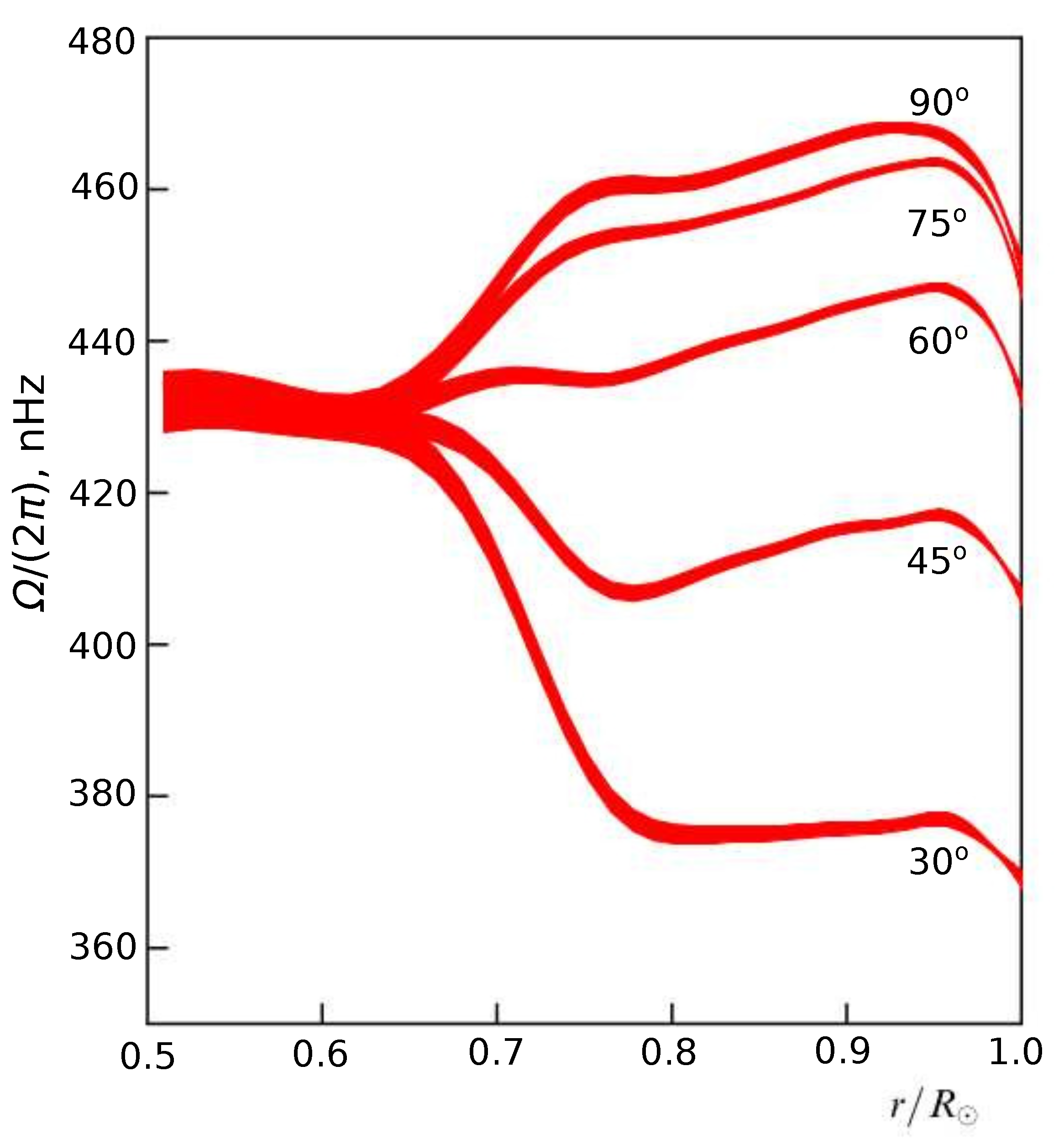
The velocity–depth structure is obtained using helioseismology methods. Results of the corresponding experiments are illustrated in Figure 1, where the ordinate of the point ${\displaystyle \frac{\Omega }{2\pi }}$ is plotted.

It is clear from Figure 1 that in the depth range of $0.65\le r\le 1$, there is a clear dependence on colatitude $\theta$. In the range of $0.5\le r<0.65$, there is only radial dependence. For the depths $r<0.5$ in the radiative zone, we can accept the angle velocity constant value [12].

In order to combine the distribution of angular velocity on the surface (19) with the distribution by depth for $0.65\le r\le 1$ from Figure 1, we introduce the model distribution

$${\displaystyle \frac{\Omega (r,\theta )}{2\pi }}=a\left(r\right)+b\left(r\right){cos}^2\theta +c\left(r\right){cos}^4\theta ,$$

(21)

where $a\left(r\right)$, $b\left(r\right)$, and $c\left(r\right)$ are some radial functions with a frequency dimension.

Then, distribution (21) at $r=1$ will coincide with (19) and (20) if

$$\begin{array}{c}{\displaystyle a\left(1\right)=\frac{{\Omega }_0}{2\pi }=456.7747\mathrm{nHz},b\left(1\right)=-\frac{\widehat{b}·{\Omega }_0}{2\pi }=-54.813\mathrm{nHz},}\hfill \\ {\displaystyle c\left(1\right)=-\frac{\widehat{c}·{\Omega }_0}{2\pi }=-77.6517\mathrm{nHz}.}\hfill \end{array}$$

(22)

From Figure 1, it is clearly seen that $\Omega (r,\theta )/\left(2\pi \right)=430$ nHz for any $\theta$ and on some branches there are two obvious extremum points. Therefore, as approximations for $a\left(r\right)$, $b\left(r\right)$, and $c\left(r\right)$ we use polynomials of the fourth degree. Such polynomials have enough degrees of freedom to ensure the existence of two extrema and given values $r=1$ and $r=0.65$. So, we use the following model expressions:

$${\displaystyle \begin{array}{c}{\displaystyle a\left(r\right)=456.7747+a_1\left(r-1\right)+a_2{\left(r-1\right)}^2+a_3{\left(r-1\right)}^3+a_4{\left(r-1\right)}^4,}\hfill \\ b\left(r\right)=-54.813+b_1\left(r-1\right)+b_2{\left(r-1\right)}^2+b_3{\left(r-1\right)}^3+b_4{\left(r-1\right)}^4,\hfill \\ c\left(r\right)=-77.6517+c_1\left(r-1\right)+c_2{\left(r-1\right)}^2+c_3{\left(r-1\right)}^3+c_4{\left(r-1\right)}^4.\hfill \end{array}}$$

(23)

Note that conditions (22) are satisfied for any constant coefficients $a_i$, $b_i$, and $c_i$.

Let us now substitute expressions (23) into (21) and require that $\Omega \left(0.65,\theta \right)/\left(2\pi \right)=430$ for all values of the angle $\theta$ from Figure 1, i.e.,

$$\begin{array}{c}{\displaystyle a\left(0.65\right)+b\left(0.65\right){cos}^2{\theta }_k+c\left(0.65\right){cos}^4{\theta }_k=430,k=1,\dots ,5,}\hfill \\ {\theta }_1=90°,{\theta }_2=75°,{\theta }_3=60°,{\theta }_4=45°,{\theta }_5=30°.\hfill \end{array}$$

(24)

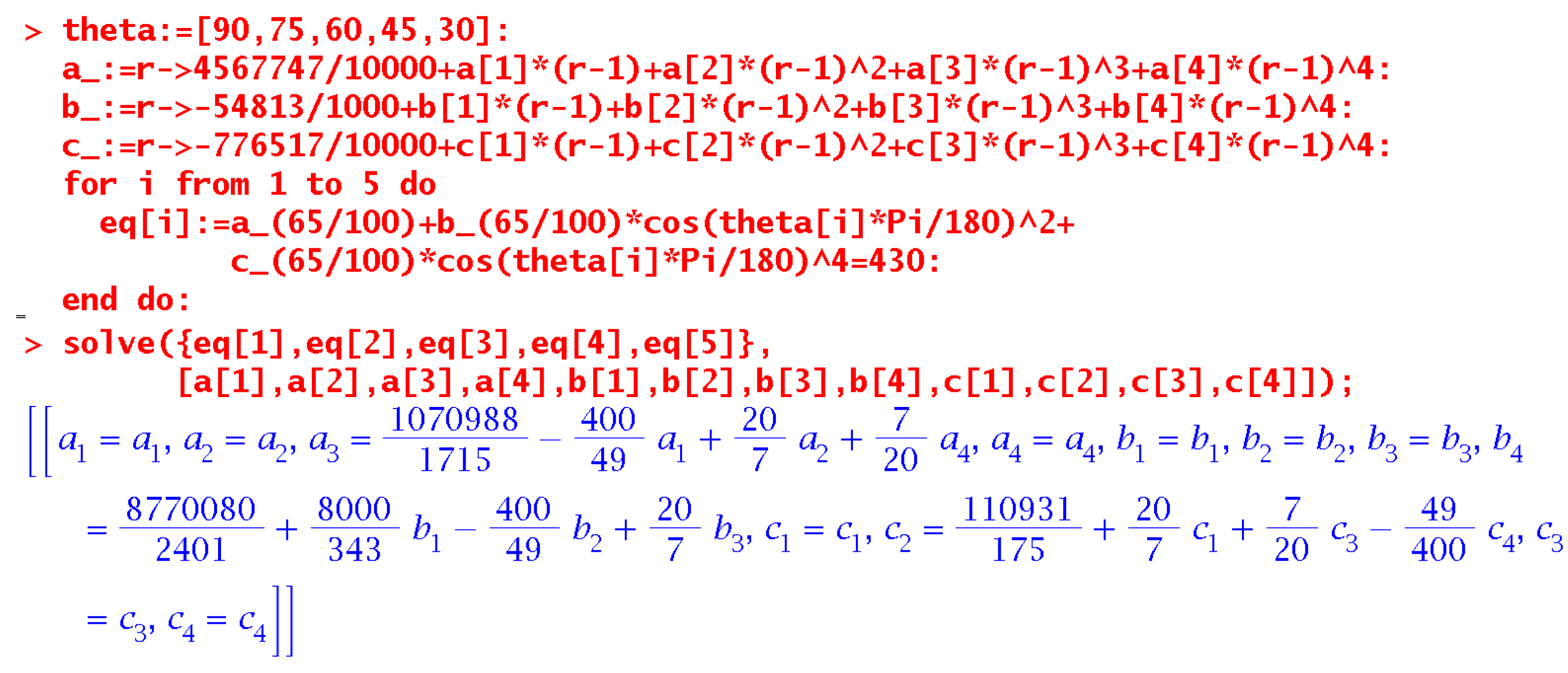
This system is underdetermined, since it contains five equations and 12 unknowns $a_i$, $b_i$, $c_i$, $i=1,\dots ,4$. To obtain its general solution, we use the Maple package. The results are shown in Figure 2. In order to obtain a general solution, the numerical data are presented as rational fractions. It is evident that in the general solution there are nine free unknowns, i.e., in the system (24) there are actually only three independent equations.

Based on the solution presented in Figure 2, we obtain the following expressions:

$$\begin{array}{c}{\displaystyle a_4=-1784.2366+23.3236a_1-8.1633a_2+2.8571a_3,}\hfill \\ {\displaystyle b_4=3652.6781+23.3236b_1-8.1633b_2+2.8571b_3,}\hfill \\ {\displaystyle c_4=5174.6239+23.3236c_1-8.1633c_2+2.8571c_3.}\hfill \end{array}$$

(25)

In the expressions $a\left(r\right)$, $b\left(r\right)$, and $c\left(r\right)$, given in Formula (23), it remains to determine the values $a_i$, $b_i$, and $c_i$, $i=1,2,3$. We will determine them using the least squares method so that function (21) approximates the dependencies shown in Figure 1. Based on this figure, we make a values table for the ${\displaystyle \frac{\Omega (r,\theta )}{2\pi }}$ with step 0.05 for r. The result of tabulation is given in

Table 1. Table of correspondences of the velocity $\Omega$ depending on the depth r and angle $\theta$.

$\mathbf{\Omega }(\mathit{r},\mathit{\theta })/\left(2\mathit{\pi }\right)$
θ\r	0.65	0.7	0.75	0.8	0.85	0.9	0.95
90°	430	447	460	461	464	467	468
75°	430	444	453	455	458	462	464
60°	430	435	435	437	441	445	447
45°	430	423	409	408	412	415	417
30°	430	410	384	376	376	376	378

.

The approximations (21) and (23) for angular velocity taking into account (25) are linear in the coefficients $a_i$, $b_i$, and $c_i$, $i=1,2,3$, so we obtain a standard least squares problem. Solving this problem and using (25) gives values for the coefficients:

$$\begin{array}{c}{\displaystyle a_1=-365.9039,a_2=-3884.8234,a_3=-15318.4868,a_4=-22372.6993,}\hfill \\ {\displaystyle b_1=67.8017,b_2=-1254.5555,b_3=-818.9596,b_4=-13135.4436,}\hfill \\ {\displaystyle c_1=-4.70435,c_2=715.3853,c_3=-5670.4067,c_4=-16976.14054.}\hfill \end{array}$$

So, we obtain an approximation Sun differential rotation at depths $0.65\le r\le 1$.

At depths $0.5\le r<0.65$, Equation (21) is not applicable, since Figure 1 shows that there is no dependence on the colatitude $\theta$. Therefore, an approximating dependence only on r is needed. It should continuously pass into (21) at $r=0.65$. In Figure 1, two extrema are visible, so we use a polynomial of degree 3 in the following form:

$${\displaystyle \frac{\Omega (r,\theta )}{2\pi }}=430+p_1(r-0.65)+p_2{(r-0.65)}^2+p_3{(r-0.65)}^3,$$

(26)

where $p_1,p_2,p_3$ are constants with a frequency dimension. This representation will provide a continuous transition to (21) at $r=0.65$. From Figure 1, it is clear that at $r=0.5$, $r=0.55$, and $r=0.6$, the value ${\displaystyle \frac{\Omega (r,\theta )}{2\pi }}$ is, respectively, equal to 432, 432, and 430.

We obtain the following equations:

$$\begin{array}{c}{\displaystyle 430-0.05p_1+0.0025p_2-0.000125p_3=430,}\hfill \\ {\displaystyle 430-0.1p_1+0.01p_2-0.001p_3=432,}\hfill \\ {\displaystyle 430-0.15p_1+0.0225p_2-0.003375p_3=432,}\hfill \end{array}$$

with solutions

$$p_1=46.667,p_2=1200,p_3=5333.333.$$

Finally, for $r<0.5$ we set the constant value ${\displaystyle \frac{\Omega }{2\pi }=432}$, taking into account the data in Figure 1.

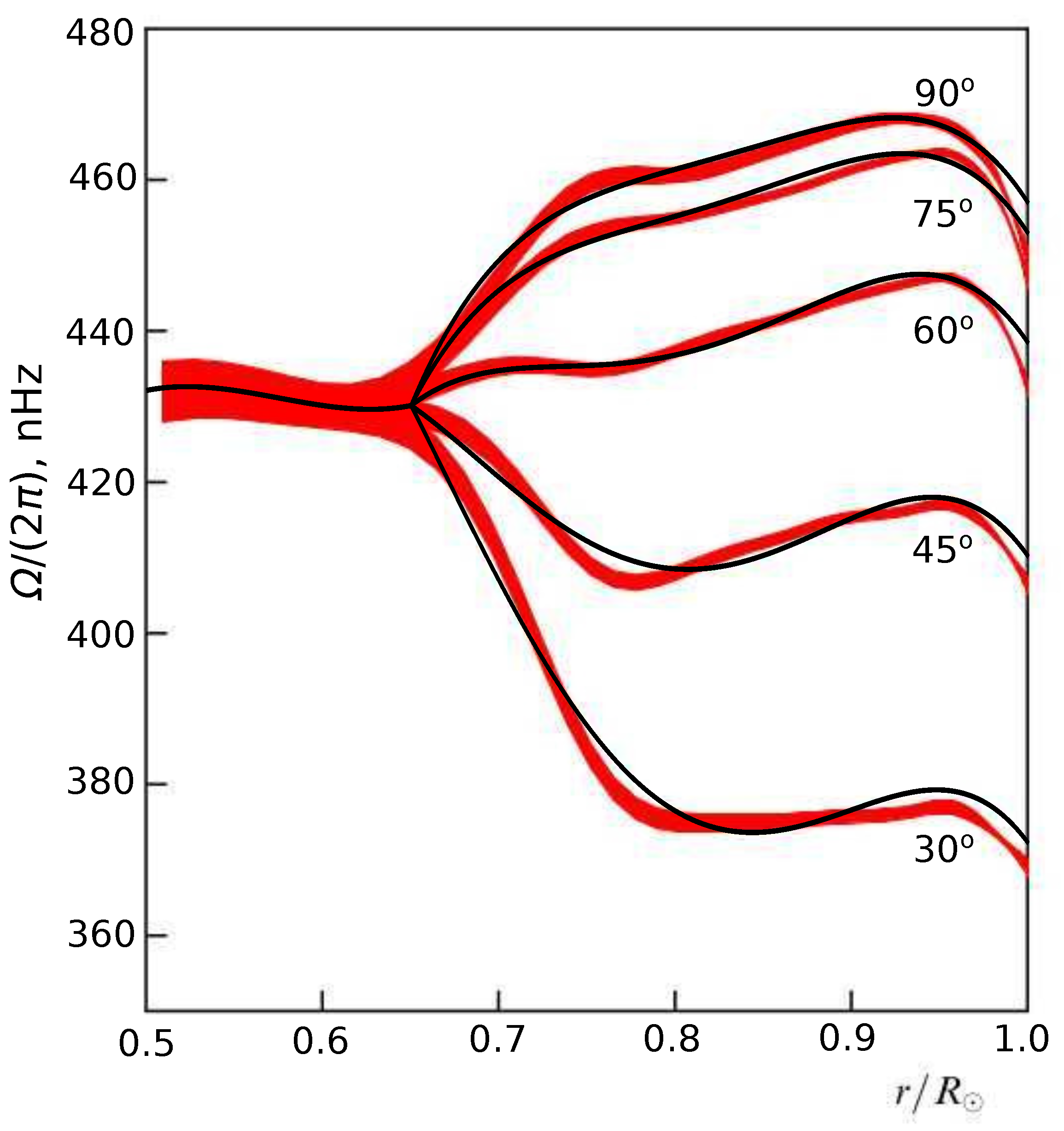
As a result of these calculations, we obtain the model distribution of angular velocity. Visual comparison of the model distribution with helioseismology data is illustrated in Figure 3. Good agreement of the model and the observed values is clear.

The constructed approximations for differential rotation were obtained based on two types of data. These are data on the non-uniformity of the solar surface rotation based on Doppler shift data and helioseismological data. Obviously, the data of the first type are more reliable, since they were obtained by direct observations. Helioseismological data are the result of complex processing and solving inverse problems. Therefore, when constructing the approximation, we required that the model distribution on the surface coincided (exactly) with Doppler measurements, and not with helioseismological data. In Figure 3, it is clearly seen that there are deviations of the model (thin lines) from the seismological data (red stripes). The authors do not have access to the digital arrays of measurements, which are presented in the works [12,18]. The authors used a graphical representation of these data from [12] (Figure 1). Therefore, it is not possible to estimate the errors of these data. Of course, the modeling results depend on the data embedded in the differential rotation model. However, we note that the expression for ${\mathbf{U}}_{\omega }$ is included in the system (12) only as part of the coefficient $\omega$ (see Formula (11)). In the system (17), ${\mathbf{U}}_{\omega }$ is included only as part of D and s, which depend on $\omega$. It is important that the value of the coefficient $\omega$ is determined as a result of integrating the expression containing ${\mathbf{U}}_{\omega }$. Such an integral in the statistical sense is a certain averaging of the differential rotation distribution. Therefore, it seems that the value of $\omega$ should not be very sensitive to errors in helioseismological data.

We also note that using the least squares method when constructing the approximation also reduces the sensitivity to errors.

4. Magnetic Modes

To represent the Sun’s magnetic field as modes ${\mathbf{b}}^T$ and ${\mathbf{b}}^P$, we use two eigen modes of magnetic field free decay in a single conducting ball, i.e., solution of a spectral problem,

$$\begin{array}{c}{\displaystyle \Delta {\mathbf{B}}^T+{\eta }^T{\mathbf{B}}^T=0,\Delta {\mathbf{B}}^P+{\eta }^P{\mathbf{B}}^P=0,}\hfill \end{array}$$

with corresponding boundary conditions (7). Free decay modes have the following form [13,19]:

• Toroidal

  $$\begin{array}{c}{\displaystyle {\mathbf{B}}_{knm}^T\left(\mathbf{r}\right)=rot\left(R_{kn}^T\left(r\right)Y_n^m\left(\theta ,\phi \right)\mathbf{r}\right),}\hfill \\ {\displaystyle R_{kn}^T=a_{kn}^T{j}_n\left(\sqrt{{\eta }_{kn}^{T}r}\right),}\hfill \\ {\displaystyle k=0,1,\dots ,n=1,2,3,\dots ,m=-n\dots n,}\hfill \end{array}$$

  (27)

  where $j_n(·)$ are the spherical Bassel functions of the first kind, $Y_n^m\left(\theta ,\phi \right)$ are the spherical harmonics, ${\eta }_{kn}^T>0$ are the eigen values, and $a_{kn}^T$ are the normalization factors;
• Poloidal

  $$\begin{array}{c}{\displaystyle {\mathbf{B}}_{knm}^P\left(\mathbf{r}\right)=rotrot\left(R_{kn}^P\left(r\right)Y_n^m\left(\theta ,\phi \right)\mathbf{r}\right),}\hfill \\ {\displaystyle R_{kn}^P=a_{kn}^P{j}_n\left(\sqrt{{\eta }_{kn}^{P}r}\right),}\hfill \\ {\displaystyle k=0,1,\dots ,n=1,2,3,\dots ,m=-n\dots n.}\hfill \end{array}$$

  where ${\eta }_{kn}^P>0$ are the eigen values and $a_{kn}^P$ are the normalization factors.

Spherical functions in real-valued form $Y_n^m\left(\theta ,\phi \right)$

$${\displaystyle Y_n^m\left(\theta ,\phi \right)=\left\{\begin{array}{c}{P}_n^{-m}\left(cos\theta \right)cos\left(-m\phi \right)m\le 0,\hfill \\ P_n^m\left(cos\theta \right)sin\left(m\phi \right)m>0,\hfill \end{array}\right.}$$

where $P_n^m\left(cos\theta \right)$ are the associated Legendre polynomials normalized such that

$$\begin{array}{c}{\displaystyle {\int }_0^{\pi }sin\theta d\theta {\int }_{-\pi }^{\pi }{\left(Y_n^m(\theta ,\phi )\right)}^{2}d\phi =1.}\hfill \end{array}$$

For the problem of axisymmetric dynamo, it is necessary to use the modes from $m=0$. Calculation schemes for eigen values and normalization factors are described in detail in the paper [19]. This paper also presents initial codes of software in the Maple package.

We choose two modes of free decay for model construction. The standard scheme of Parker’s dynamo [1] assumes that the toroidal component is formed from the poloidal one due to the differential rotation. It is clear from geometry that toroidal mode force lines should be oppositely directed in northern and southern hemispheres. The largest-scale toroidal eigen mode of such a type is ${\mathbf{B}}_{020}^T$, with the eigen value ${\eta }^T=33.48$. Thus, we assume that in the decomposition (8) ${\mathbf{b}}^T={\mathbf{B}}_{020}^T$. As the poloidal mode, we use one of the dipole modes of the kind $B_{k10}^P$. For the first three such modes, the eigen values are equal to $9.8696$, $39.47841$, and $88.82643$. The eigen values determine the characteristic time of mode dissipation. For the two components in the model to have close dissipation times, we apply the mode ${\mathbf{B}}_{110}^P$ as ${\mathbf{b}}^P$ in the decomposition (8).

It is known that the Sun’s poloidal magnetic field, in addition to a strong dipole component, also contains a strong quadrupole component [8]. More precisely, during the minimum of solar activity, the field is mainly dipole, and during the maximum, mainly quadrupole. In order to describe this change in the field structure, it is necessary to introduce at least two poloidal modes, and then at least two toroidal modes associated with them by the geometric structure of the field lines should also be taken. This is no longer possible to implement within the framework of the two-mode approximation. Therefore, we took the dipole mode, as a simpler one, in order to explore the very idea of the model with memory. In addition, such a mode better reflects the original scheme of Parker’s dynamo [4]. It is clear that it is also possible to construct a two-mode model based on the quadrupole poloidal mode and a suitable toroidal mode. Conjugation of such models in further studies is also promising.

Thus, in the case of the solar dynamo, we consider the following components:

$$\begin{array}{c}{\displaystyle {\mathbf{b}}^T={\mathbf{B}}_{020}^T=a_{02}^T{j}_2\left(\sqrt{{\eta }_{02}^{T}r}\right)\left(\frac{3\sqrt{5}cos\left(\theta \right)sin\left(\theta \right)}{2\sqrt{\pi }}\right){\mathbf{e}}_{\phi },}\hfill \\ {\displaystyle a_{02}^T=3.48752,}\hfill \\ {\displaystyle {\eta }_{02}^T=33.21746,}\hfill \\ {\displaystyle {\mathbf{b}}^P={\mathbf{B}}_{110}^P=a_{11}^P{j}_1\left(\sqrt{{\eta }_{11}^{P}r}\right)\left(\frac{\sqrt{3}cos\left(\theta \right)}{r\sqrt{\pi }}\right){\mathbf{e}}_r-}\hfill \\ {\displaystyle -\frac{a_{11}^P\sqrt{3}sin\left(\theta \right)}{2\sqrt{\pi }}\left(\frac{j_1\left(\sqrt{{\eta }_{11}^{P}r}\right)+\sqrt{{\eta }_{11}^P}{j}_1^{\prime }\left(\sqrt{{\eta }_{11}^{P}r}\right)r}{r}\right){\mathbf{e}}_{\theta },}\hfill \\ {\displaystyle a_{11}^P=1,}\hfill \\ {\displaystyle {\eta }_{11}^P=39.478417.}\hfill \end{array}$$

In these formulas, the numerical normalization factors and eigen values were obtained by the software complex described in the papers [19,20]. We should note that normalization factor values provide the condition $\parallel {\mathbf{b}}^T\parallel = \parallel {\mathbf{b}}^P\parallel = 1$.

We now turn back to the coefficients (11). As the approximation of the $\alpha$-effect for the Sun, it is generally accepted to use the expression [21]

$$\alpha =rcos\theta .$$

Then, the coefficients (11) take the form

$$\begin{array}{c}{\displaystyle \omega =0.0292,{\alpha }^T=0.6087,{\alpha }^P=0.2156,}\hfill \\ {\displaystyle {\eta }^T={\eta }_{02}^T=33.2175,{\eta }^P={\eta }_{11}^P=39.4784.}\hfill \end{array}$$

On the basis of the obtained coefficients of generators and dissipation, we can estimate the relative dynamo number D.

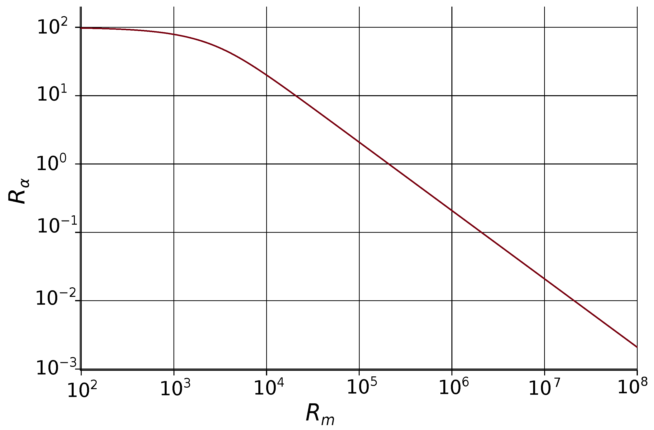
Let us now carry out numerical simulation. Now, we consider the threshold condition for field generation, i.e., $D=1$ or

$${\displaystyle \left(R_{\alpha }{\alpha }^T+R_m\omega \right)R_{\alpha }{\alpha }^P={\eta }^T{\eta }^P.}$$

(28)

We express $R_{\alpha }$ in terms of $R_m$ from (28), taking into account $R_{\alpha }>0$. The corresponding expression has the form

$$R_{\alpha }={\displaystyle \frac{\sqrt{\left({\left(R_m{\alpha }^P\omega \right)}^2+4{\alpha }^T{\alpha }^P{\eta }^T{\eta }^P\right)}-R_m{\alpha }^P\omega }{2{\alpha }^T{\alpha }^P}}.$$

This dependence graph is illustrated in Figure 4.

The following values are typical for the Sun dynamo: $R_m={10}^8$ and $R_{\alpha }=0.5$ [16,22]. We substitute the values $R_m$ and $R_{\alpha }$ into Equation (Figure 4). As a result, we obtain the following value of the number $D=239.86318$. Now, we calculate other coefficient values for the system (17), in particular the values

$${\displaystyle \eta =0.84140,s=0.00001,\xi =2.82320.}$$

We should note that the product $\xi s^2$ that determines the intensity of the $\alpha$-generator for the toroidal component in (17) is a vary small number $\sim {10}^{-10}$. Thus, this term can be neglected and we consider that the Sun magnetic field generation can be described by the model of $\alpha \omega$-dynamo.

5. Difference Scheme

Now, we will describe the difference scheme that was used for the numerical solution of the problem (17) and (18).

This problem can be written in the following general form:

$$\begin{array}{c}{\displaystyle \frac{d\mathbf{x}}{dt}=\mathbf{f}\left(\mathbf{x},z,\mathbf{a}\right),z\left(t\right)={\int }_0^{t}K\left(t-\tau \right)Q\left(\mathbf{x}\left(\tau \right)\right)d\tau ,\mathbf{x}\left(0\right)={\mathbf{x}}_0,}\hfill \end{array}$$

(29)

where $\mathbf{x}\left(t\right)={\left[x_1\left(t\right),x_2\left(t\right)\right]}^T$, $z\left(t\right)=x_3\left(t\right)$, $\mathbf{a}={\left[{\eta }^T,{\eta }^P,\xi ,s,D\right]}^T$.

Let us introduce the time grid $\left\{t^n\right\}$ with a step h and let $\mathbf{x}\left(t^n\right)={\mathbf{x}}^n$, $z\left(t^n\right)=z^n$, and $K\left(t^n\right)=K_n$. To solve the problem (29), a “predictor–corrector”-type difference scheme was used:

$${\displaystyle \begin{array}{l}{\mathbf{x}}^{pr}={\mathbf{x}}^n+h\mathbf{f}({\mathbf{x}}^n,z^n,\mathbf{a}),\\ L_n=\{\begin{array}{ll}n=0& 0,\\ n>0,& \frac{h}{2}{K}_{n+1}Q\left({\mathbf{x}}^0\right)+h{\displaystyle \sum _{i=1}^{n-1}}{K}_{n+1-i}Q\left({\mathbf{x}}^i\right)+\frac{h}{2}{K}_{1}Q\left({\mathbf{x}}^n\right),\end{array}\\ z^{pr}=L_n+h{K}_{1}Q\left({\mathbf{x}}_n\right),\\ {\mathbf{x}}^{n+1}={\mathbf{x}}^n+\frac{h}{2}(\mathbf{f}({\mathbf{x}}^n,z^n,\mathbf{a})+\mathbf{f}({\mathbf{x}}^{pr},z^{pr},\mathbf{a})),\\ z^{n+1}=L_n+\frac{h}{2}(K_{1}Q\left({\mathbf{x}}^n\right)+K_{0}Q\left({\mathbf{x}}^{pr}\right)).\end{array}}$$

(30)

For the differential part of the problem, this scheme is based on the improved Euler method, and for the integral part, the trapezoidal rule.

6. Simulations

In order to apply models of the type (17) to the description of the solar dynamo, it is necessary to specify the form of the kernel $K\left(t\right)$ and the quadratic form $Q(x_1,x_2)$. In the work [23], an axisymmetric model of the solar dynamo was proposed, in which the influence of the magnetic field on the $\alpha$-effect was described by the classical Lorenz system. If we write the model of the work [23] in the notation of the system (17), then this model has the form

$$\begin{array}{c}{\displaystyle \frac{d{x}_1}{dt}=\frac{{\eta }^T}{{\eta }^P}{x}_2-\frac{{\eta }^T}{{\eta }^P}{x}_1,}\hfill \\ {\displaystyle \frac{d{x}_2}{dt}=(D-x_3)x_1-x_2,}\hfill \\ {\displaystyle \frac{d{x}_3}{dt}=x_1{x}_2-b{x}_3.}\hfill \end{array}$$

(31)

It is evident that (31) differs from our (17) by the last equation. However, it is easy to show that the third equation of the system (17) in the case of the kernel $K\left(t\right)=e^{-bt}$ will be equivalent to the equations

$$\begin{array}{c}{\displaystyle \frac{d{x}_3}{dt}=Q\left(x_1,x_2\right)-b{x}_3,x_3\left(0\right)=0.}\hfill \end{array}$$

Therefore, we can say that the model proposed in [23] is a special case of ours (17) with $K\left(t\right)=e^{-bt}$ and $Q(x_1,x_2)=x_1{x}_2$. In this regard, the kernel $K\left(t\right)=e^{-bt}$ can be used to describe the solar dynamo. This is a kernel with rapidly disappearing exponential memory.

The paper [7] was already mentioned in the Introduction. In this paper, it was shown that the simultaneous values of the $\alpha$-effect and the magnetic field are uncorrelated. In the model (17), this should mean that $x_3\left(t\right)$ should depend on $Q\left(x_1\left(\tau \right),x_2\left(\tau \right)\right)$ only when $\tau <t$, which means $K\left(0\right)=0$. In this case, the exponential kernel must be modified, for example in the form $K\left(t\right)=t^n{e}^{-bt}$. The long-term correlation in [7] can also be taken into account using a slowly decaying power-law kernel.

Taking all these considerations into account, further in this paper we consider two different types of kernels of a quenching integral; they are as follows: kernels with exponential asymptotics $K\left(t\right)=t^n{e}^{-bt}$ and kernels with power symptotics ${\displaystyle K\left(t\right)=\frac{t^n}{{(1+t)}^{b+n}}}$, where $n=0,1,2,3\dots$. Here $b^{-1}>0$ determines the kernel time scale. It is clear that when $K\left(0\right)\ne 0$, an immediate response in feedback coupling occurs. If $K\left(0\right)=0$, there is a response delay. The parameter n value determines the presence of a delay ($n\ne 0$) or its absence ($n=0$). Moreover, as n grows, the kernel maximum point increases, and this is why zero n determines the delay value, since quenching slightly depends on field component values at the times close to the present moment.

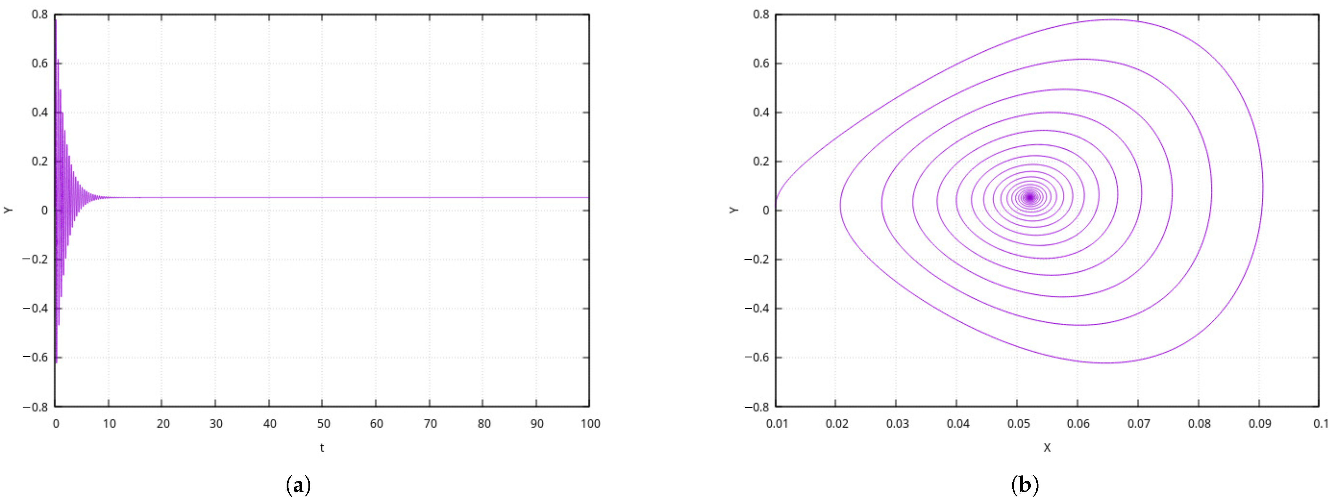
First, we consider the case for $n=0$ and choose field helicity, in particular $Q(x_1,x_2)=x_1{x}_2$, as the function of $\alpha$-effect quenching. As the kernel of the integral operator $K\left(t\right)$, we take the one with exponential asymptotics. As a result, we obtain

$$K\left(t\right)=e^{-bt}.$$

Figure 5 shows the modeling results when $b=1$. This figure and the following ones show phase trajectories and the phase coordinate $y\left(t\right)$. This coordinate corresponds to model representation of the Sun’s poloidal field. The real poloidal field can be observed directly. The second phase coordinate $x\left(t\right)$ corresponds to the field toroidal component. This component is hidden inside the Sun and is inaccessible for direct observations. Thus, we will further analyze the time dynamics of the poloidal component.

It is clear from Figure 5 that for the exponential kernel with immediate response, quick onset of an asymptotically stationary regime occurs after a short transition process. Such a behavior is not typical for the Sun’s field, in which a number of cycles (22-year and secular) are known [8].

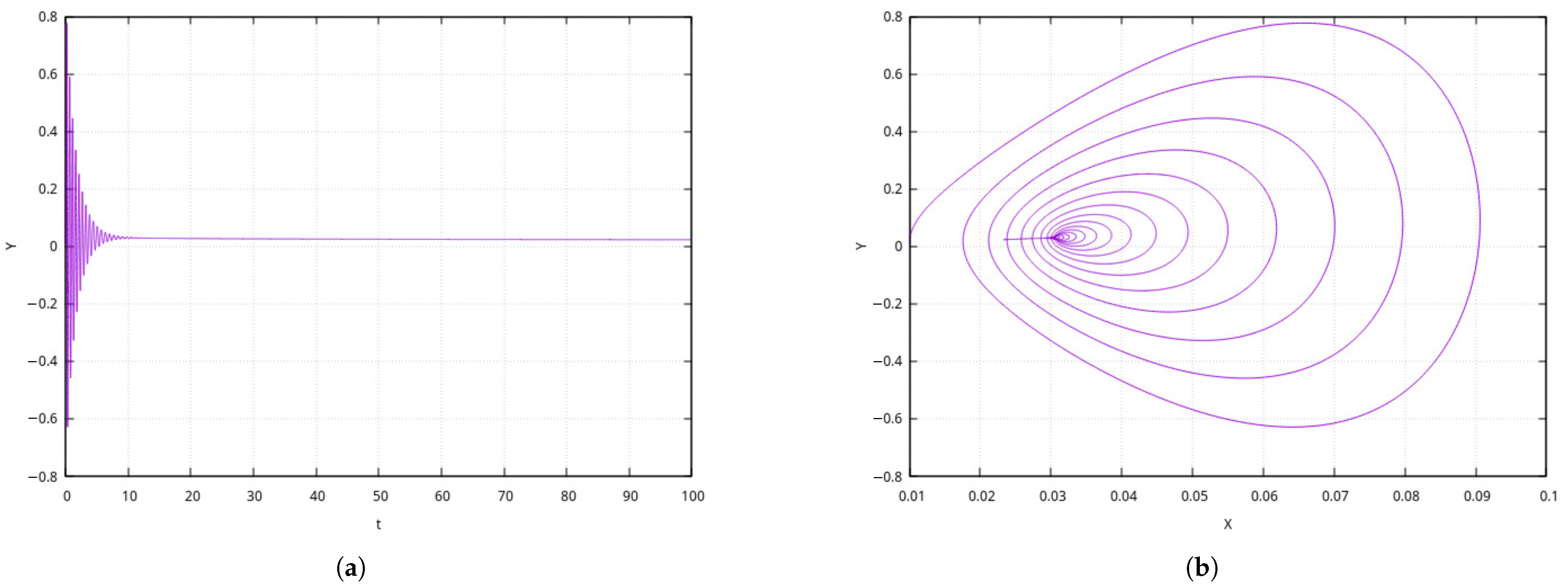
Now, we consider the case of the power kernel, i.e., we assume that ${\displaystyle K\left(t\right)=\frac{1}{{(1+t)}^b}}$. Figure 6 shows the modeling results for $b=1$ as well. Here, the asymptotic stationary regime, not typical for the Sun, is also clearly seen.

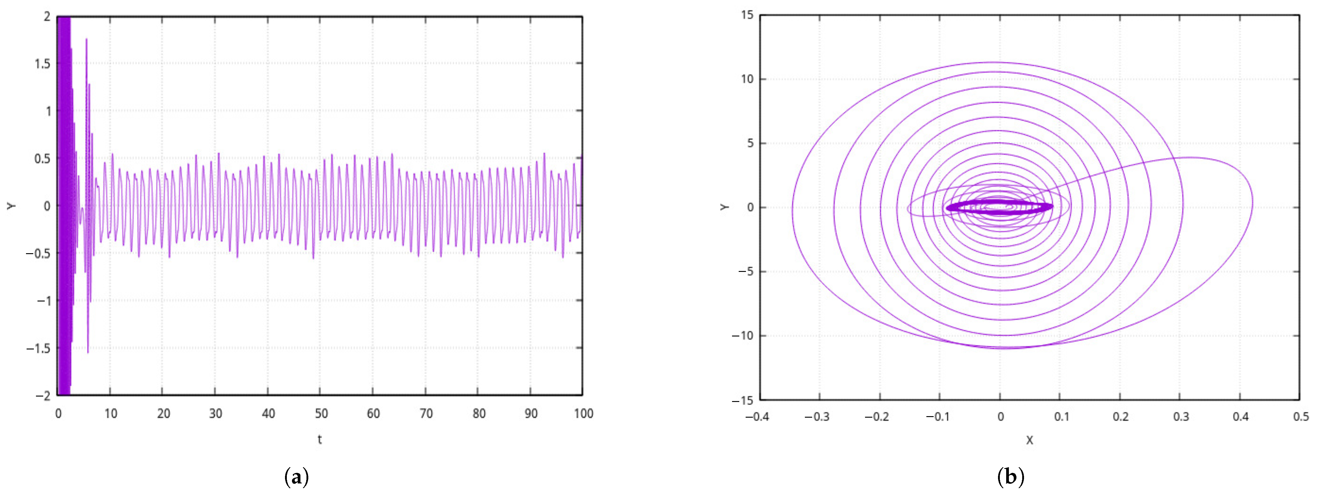
The previous examples were estimated for the kernels, reflecting the immediate feedback effect of the turbulent generator of the $\alpha$-effect on the magnetic field components. Now, we consider the kernels corresponding to the delay in the feedback. In order to achieve this, we take the parameter $n=1$.

First, we take $K\left(t\right)=t{e}^{-bt}$ as the kernel. The modeling result is illustrated in Figure 7. Here, after the transition process, there is a short interval of generation weakening ($5\le t\le 8$), and then a short stage of growth followed by a stable quasiperiodic regime. Such a situation agrees well with the known regimes of solar activity, such as solar cycles and the Maunder minimum [8].

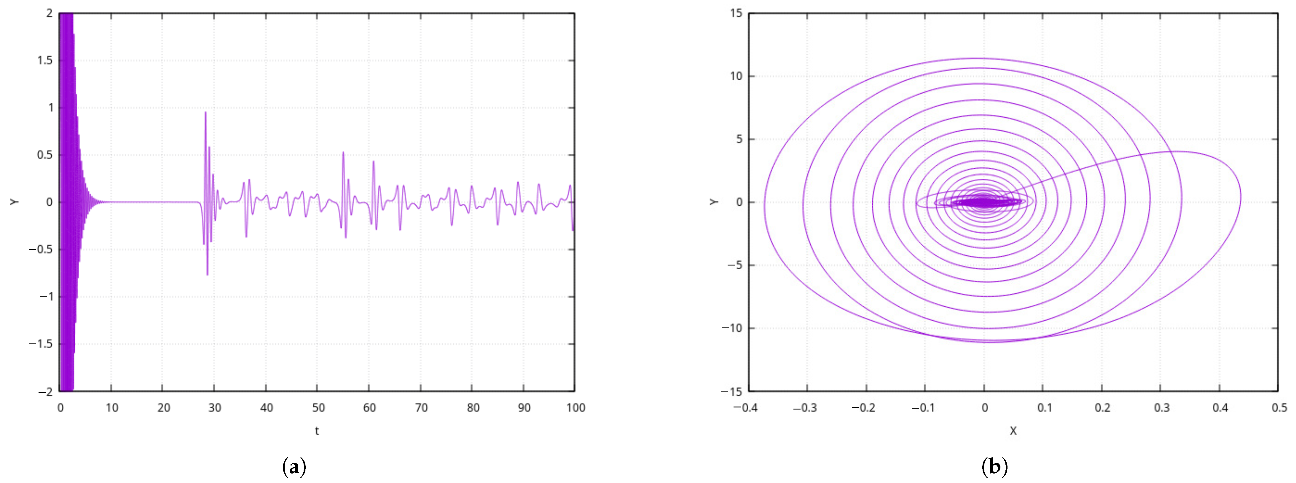
The kernel ${\displaystyle K\left(t\right)=\frac{t}{{(1+t)}^{b+1}}}$ is considered in a similar way. The result is illustrated in Figure 8. Here, we see the generation regime of a chaotic outburst type. Such regimes are not typical for the Sun; however, they are known in real dynamo systems [1].

7. Conclusions

In the present paper, a two-mode model of hydromagnetic dynamo with memory was suggested. The model describes two mechanisms of large-scale field component generation: generation due to the medium differential rotation ($\omega$-effect) and generation due to the nonlinear interaction of small-scale turbulent pulsations ($\alpha$-effect). In real dynamo system, the Lorenz force represents the feedback connection by adjusting the field generator’s performance. In the model, this feedback is introduced phenomenologically as $\alpha$-effect quenching by field helicity. This quenching is determined not only by helicity’s real value but by the previous values as well. Thus, dynamic memory is introduced into the model.

It is known that memory plays an important role in the dynamo theory and turbulence theory. In the numerical simulation of detailed scale dynamo models, delays in the feedback in the system were also observed. It turned out that the simultaneous values of the $\alpha$-effect and the field are uncorrelated.

The model proposed in this work allows one to take into account both of these effects by choosing the quenching kernel. It is the kernel that allows one to vary such properties of the model as the absence or presence of a delay and the duration of the delay, the absence or presence of an effective memory duration, and its value. In addition, the introduction of the memory functional in a certain sense increases the dimensionality of the phase space of the model. As a consequence, this leads to the emergence of complex dynamic regimes, such as chaos, which cannot exist in classical two-mode nonlinear models with algebraic quenching.

The model is used to describe the Sun dynamo. For this purpose, we built a model representation of the Sun’s differential rotation on the basis of experimental data of helioseismology, i.e., the distribution of rotation angular velocity in the model corresponds to the real one. Eigen modes of magnetic field free decay are used as magnetic components of the two-mode model. Such modes form a physically natural basis.

Dynamic regimes were numerically modeled varying the kernel of the memory functional. Kernel types corresponded to the limited and unlimited memory time and the presence or absence of feedback delay. It turned out that dynamic regimes, typical for the Sun, occur in the case of limited memory with a delay.

Let us discuss the limitations associated with the model. First of all, the model is constructed in the mean-field approximation, when large-scale solar fields are assumed to be axisymmetric. This is indeed the case in the first approximation. According to the authors, taking into account three-dimensional effects within the two-mode model is excessive. It makes sense to consider such effects in more spatially detailed models, which can no longer be low-mode.

We also note that the model did not take into account large-scale meridional circulation. It is clear that it is necessarily present, since even the Coriolis drift of differential rotation alone excites meridional transport. However, the meridional circulation does not lead to mutual generation of the toroidal and poloidal field components. It only corrects each of the components. Therefore, taking into account such a velocity component is secondary.

Only one poloidal mode can be used in the model if the idea of two modes is preserved. In the described model, the dipole mode was used as the poloidal mode. It is known that the dipole or quadrupole modes dominate in the Sun during different periods of activity. The impossibility of combining them is another limitation of the model.

The developed approach could be applied to other stars. But the problem is the lack of data on the distribution of differential rotation in them. The same can be said about the gas giant planets. In the case of the terrestrial planets, differential rotation is not the dominant large-scale type of motion. For such planets, it is necessary to take into account magnetoconvection in the liquid core, and this is a completely different class of models. Therefore, the application of the model approaches to other stars can only be considered at a qualitative level.

The simulation results show that a delay in the quenching of the $\alpha$-effect is necessary to reproduce solar-type solutions. If there is no such delay, then the solutions after a short transient process pass into a steady-state mode. Such field behavior is completely atypical for the Sun. At the same time, the exponential kernel better reproduces quasiperiodic modes (like the 22-year cycle) with a chaotic component, and the power kernel gives attenuation (like the Maunder minimum) and chaotic bursts. Such complex modes were obtained in the two-mode model of the solar dynamo precisely due to the memory taken into account.

Let us consider some possible further development options for the model. The model used a dipole mode, which dominates in the poloidal component of the Sun’s field during periods of minimum solar activity. At maximum activity, the quadrupole mode begins to dominate. Therefore, it is advisable to study a model in which there will be a quadrupole poloidal mode and a toroidal mode associated with it by a geometric structure. A transition to models in which a quadrupole mode will be present in addition to the dipole mode is also possible. This will better reflect the structure of the solar magnetic field, but will require a transition to three- or four-mode models. The appearance of the fourth mode may be due to the fact that one toroidal mode may not be sufficient to generate poloidal modes with dipole and quadrupole symmetry.

In the future, it will also be possible to try to combine two types of asymptotics of quenching kernels to obtain transitions between dynamic modes in one two-mode model.

A separate direction may be the study of the sensitivity of the model to errors in determining the distribution of differential rotation, for example, using random disturbances of helioseismological data.