Using Physics-Informed Neural Networks for Modeling Biological and Epidemiological Dynamical Systems

Abstract

Physics-Informed Neural Networks (PINNs) have emerged as a powerful approach for integrating physical laws into a deep learning framework, offering enhanced capabilities for solving complex problems. Despite their potential, the practical implementation of PINNs presents significant challenges. This paper explores the application of PINNs to systems of ordinary differential equations (ODEs), focusing on two key challenges: the forward problem of solution approximation and the inverse problem of parameter estimation. We present three detailed case studies involving dynamical systems for tumor growth, gene expression, and the SIR (Susceptible, Infected, Recovered) model for disease spread. This paper outlines the core principles of PINNs and their integration with physical laws during neural network training. It details the steps involved in implementing PINNs, emphasizing the critical role of network architecture and hyperparameter tuning in achieving optimal performance. Additionally, we provide a Python package, ODE-PINN, to reproduce results for ODE-based systems. Our findings demonstrate that PINNs can yield accurate and consistent solutions, but their performance is highly sensitive to network architecture and hyperparameters tuning. These results underscore the need for customized configurations and robust optimization strategies. Overall, this study confirms the significant potential of PINNs to advance the understanding of dynamical systems in biology and epidemiology.

1. Introduction

Physics-Informed Neural Networks (PINNs) represent an innovative approach that integrates physical laws directly into the training of neural networks [1,2,3,4]. Unlike traditional neural networks [5,6,7,8,9,10], which rely solely on data-driven methods, PINNs incorporate knowledge of differential equations—such as Ordinary Differential Equations (ODEs) [11,12] or Partial Differential Equations (PDEs) [13,14]—into the neural network (NNs) model. This integration allows PINNs to utilize both empirical data and established physical principles, providing solutions that are consistent with known equations governed by physical laws.

The relevance of PINNs in solving differential equations is significant, particularly in modeling physical phenomena where these equations describe the evolution of quantities over time or space. Examples include heat flow, fluid dynamics [1,15,16,17,18], energy systems [19,20], material deformation [21,22,23], and geophysics [24,25,26].

Unlike traditional numerical methods such as the finite element method (FEM) or finite difference method (FDM) [27], which can be computationally intensive, especially in high-dimensional problems, PINNs offer a more flexible and data-adaptive approach by embedding the governing physical laws directly into the loss function of a neural network. While classical analytical and numerical techniques remain foundational, their effectiveness diminishes in settings involving sparse data, uncertain parameters, or partially known models. In such cases, PINNs provide a compelling alternative capable of approximating solutions without extensive preprocessing or complex numerical setups [1,3,28].

Many studies have examined the accuracy and computational efficiency of PINNs in comparison to traditional numerical methods such as the Finite Element Method (FEM). For instance, Grossmann et al. [29] conducted a comprehensive comparison and found that although PINNs can offer faster evaluation for some problems, they generally fall short of FEM in terms of overall solution accuracy and computational time. In contrast, Stiasny and Chatzivasileiadis [30] demonstrated that for specific applications like power system dynamics, PINNs can outperform traditional solvers in speed—being 10 to 1000 times faster—while still maintaining sufficient numerical accuracy and stability. However, as noted by Markidis [31], PINNs tend to converge quickly for low-frequency components but require significantly more training to accurately resolve high-frequency features, suggesting that hybrid approaches may be beneficial. Li [32] further emphasized the strengths of PINNs in modeling complex, high-dimensional systems and incorporating physical laws into data-driven models, but also highlighted challenges such as computational overhead and reduced precision in certain scenarios. Overall, while PINNs show strong potential in flexibility and speed for specific problems, traditional methods remain more reliable for achieving high accuracy and efficiency in well-posed, structured settings.

PINNs have demonstrated considerable success in applications related to physical problems. Specifically, they have been effectively used to tackle problems in fluid dynamics, heat transfer, and wave propagation. The advantages of PINNs in these areas include their ability to achieve accurate solutions with relatively sparse data, their flexibility in handling complex geometries and boundary conditions, and their capacity for generalization across various conditions once the model has been trained.

While PINNs were originally designed for and predominantly applied to physics-related problems, their potential extends beyond traditional physics applications. Instead, they can be used for general dynamical systems. However, dynamical systems often involve complex interactions and behaviors that are not fully captured by physics alone. For instance, biological processes such as tumor growth [33] and gene expression [34,35] are governed by differential equations but are influenced by complex, variable factors that are not described by physical laws. Similarly, epidemiological models like the SIR (Susceptible, Infected, Recovered) model for disease spread are described by ODEs without a connection to physics. Still, they can benefit from PINNs to improve prediction accuracy and inform public health strategies [36,37,38,39]. Furthermore, adaptive systems, including economic markets and ecological systems, could leverage PINNs to understand dynamic behavior and enhance predictive capabilities.

The aim of this paper is to demonstrate the application of PINNs in the context of Ordinary Differential Equations (ODEs), extending their use beyond traditional physics-based problems. Specifically, we focus on applications in biology, systems biology, and epidemiology, where problems are formulated as systems of ODEs. Through numerical examples, we explore how PINNs can effectively address complex challenges in dynamical systems by approximating solutions to forward problems and estimating parameters in inverse problems. This work addresses a significant gap in the literature by applying PINNs to broader systems outside of physics.

We concentrate on three models: tumor growth, gene expression, and the SIR model. For tumor growth, we investigate how PINNs can model cancer progression and predict growth patterns using differential equations that represent relevant biological processes. In the case of gene expression, PINNs are used to predict gene activity and interactions through equations capturing biological regulatory mechanisms. For disease spread, as modeled by the SIR (Susceptible, Infected, Recovered) framework, we explore how PINNs can improve our understanding of disease dynamics and enhance parameter estimation for better predictive accuracy. To make the results fully reproducible, the code of our analysis and datasets associated with this paper can be found on GitHub at https://github.com/AmerFarea/ODE-PINN (accessed on 10 May 2025).

Overall, this study illustrates the potential of PINNs to advance the understanding and modeling of complex dynamical systems, providing accurate solutions and insights that extend beyond traditional physics applications. Our exploration highlights the practical benefits of PINNs in diverse fields, contributing to the development of more adaptable and sophisticated modeling techniques.

This paper is organized as follows: We start by explaining the motivation for our study. Section 2 provides the theoretical background, covering PINNs, ODE-based dynamical systems, and forward and inverse problems. Section 3 details the experimental setup, including the implementation steps for solving forward and inverse problems to approximate solutions and estimate parameters. Section 4 presents our numerical results, followed by a discussion. Finally, the paper finishes with concluding remarks.

Motivation

When reviewing the literature [4], we found that PINNs have primarily been applied to physical problems. However, PINNs could also be beneficial for biological systems, as many examples involve the use of differential equations [40,41,42]. This extension is motivated by the need to address increasingly complex real-world problems governed by differential equations but falling outside the realm of physics. By applying PINNs in these new contexts, we can achieve significant benefits and improvements in problem-solving.

First, many contemporary challenges—such as modeling tumor growth, understanding gene expression, and predicting disease spread—are inherently complex and dynamic. These problems often involve non-linear interactions and high-dimensional systems, which can be difficult to capture using conventional methods. While traditional numerical approaches are powerful, they often struggle with scalability and computational efficiency in such scenarios. PINNs offer a robust alternative by directly integrating dynamic laws into the neural network training process, enabling more accurate solutions with less dependence on extensive data and computational resources.

Second, PINNs can enhance the interpretability and reliability of models in fields such as systems biology, network biology and epidemiology. For instance, in cancer research, PINNs can model tumor growth dynamics with the precision needed to predict progression and assess treatment strategies. In genomics, PINNs can elucidate the underlying mechanisms of gene regulation and expression, providing insights that are crucial for understanding genetic disorders and developing targeted therapies. Similarly, in epidemiology, PINNs can refine the SIR model to better predict and manage disease outbreaks, improving public health responses.

From a technical standpoint, PINNs offer the potential for improved parameter estimation in inverse problems. Many dynamical systems involve parameters that are not directly observable, but are crucial for accurate modeling. By applying PINNs, we can estimate these unknown parameters more effectively by incorporating both dynamic constraints and observational data. This capability is particularly valuable in complex systems where traditional methods may struggle to balance data fit with prediction accuracy.

The ability of PINNs to generalize across various conditions also presents a significant advantage. Once trained, PINNs can adapt to a range of scenarios and provide solutions for new or unseen conditions, making them highly versatile tools for dynamical systems modeling. This adaptability is crucial for addressing the ever-evolving nature of real-world problems, where conditions and parameters may change over time.

Overall, the extension of PINNs to dynamical systems beyond physics represents a significant advancement with the potential to revolutionize how we approach and solve complex real-world problems. By harnessing the power of PINNs, we can achieve more accurate, efficient, and interpretable models that are essential for advancing scientific understanding and addressing pressing challenges across various domains.

2. Theoretical Background

2.1. Physics-Informed Neural Networks (PINNs)

PINNs represent a significant advancement in the field of artificial intelligence and machine learning by integrating physical laws directly into the training process of neural networks [1,2,3,4]. Unlike traditional neural networks that learn solely from data, PINNs incorporate knowledge of underlying physical principles, such as differential equations, into their architecture. This integration allows PINNs to produce solutions that are consistent with known physical laws, improving both accuracy and generalization.

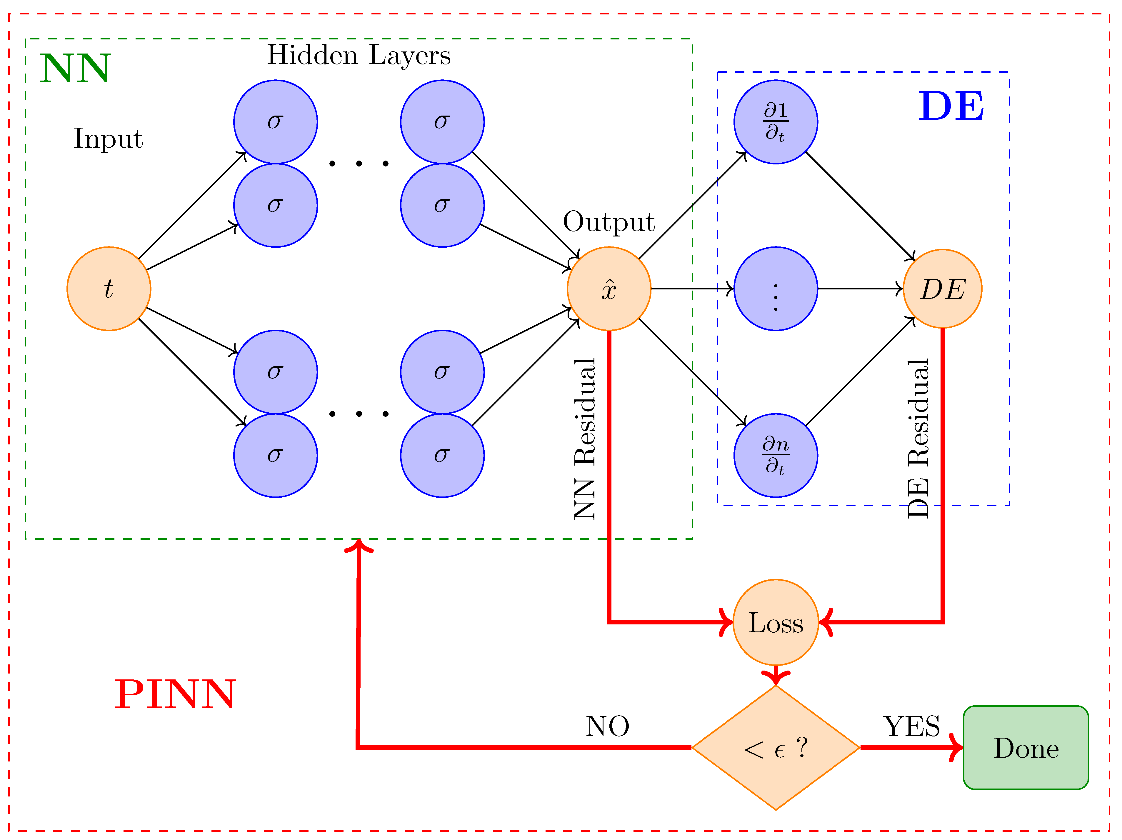
A typical PINN consists of a neural network with an architecture that includes input layers, hidden layers, and output layers. The key innovation of PINNs is the incorporation of physical constraints into the network’s loss function. Specifically, during training, PINNs optimize not only the error between the network’s predictions and the observed data but also the residuals of the governing differential equations. This approach ensures that the network’s predictions adhere to the physical laws described by the differential equations.

The training process involves minimizing a combined loss function, which typically includes a data loss term and a physics loss term. The data loss term measures the discrepancy between the predicted output and the observed data, while the physics loss term measures how well the network satisfies the differential equations that govern the system. By optimizing this combined loss function, PINNs can achieve solutions that respect both empirical data and physical laws.

2.2. ODEs-Based Dynamical Systems

Ordinary Differential Equations (ODEs) play a central role in modeling dynamical systems, which describe how quantities change over time or space according to specified rules. ODEs are used to represent a wide range of phenomena, from mechanical systems [43,44] and electrical circuits [45] to biological processes [46] and financial markets [47]. These equations encapsulate the relationships between variables and their rates of change, making them crucial for understanding and predicting system behavior.

In dynamical systems, ODEs provide a mathematical framework for describing how systems evolve over time. For example, in biological systems, ODEs can model tumor growth by capturing how the tumor size changes in response to various factors, such as treatment or natural progression. Similarly, in epidemiology, the SIR (Susceptible, Infected, Recovered) model uses ODEs to describe the spread of infectious diseases within a population. Below is a brief overview of the dynamical system utilized in this study, along with the associated differential equations.

• Tumor Growth Model
  In the 1960s, A.K. Laird [33] successfully applied the Gompertz curve [48] to model tumor growth, recognizing that tumors are cellular populations expanding in a confined space with limited nutrients. The Gompertz curve for tumor size $X\left(t\right)$ is expressed as:

  $$X\left(t\right)=Kexp\left(log\left({\displaystyle \frac{X\left(0\right)}{K}}\right)exp\left(-\alpha t\right)\right)$$

  (1)

  where $X\left(0\right)$ is the initial tumor size, K is the carrying capacity, and $\alpha$ represents the cell proliferation rate. The curve approaches K as time progresses, regardless of the initial size. The corresponding differential equation is:

  $${\displaystyle \frac{dX}{dt}}=\alpha log\left({\displaystyle \frac{K}{X\left(t\right)}}\right)X\left(t\right)$$

  (2)
  This model captures the decline in proliferation rate due to nutrient competition, similar to logistic growth [49] but with an unbounded rate for small tumors, which can be unrealistic. Recent insights suggest that the Gompertz model might not fit small tumors well and may not account for immune interactions effectively. Fornalski et al. [50] found that while the Gompertz curve fits typical cancer growth patterns, it is less accurate for very early stages, where other models might be more appropriate.
• Gene Expression Model
  The dynamics of gene expression can be modeled using differential equations that describe the behavior of mRNA and protein concentrations over time [34,35]. The rate of change of mRNA concentration is given by:

  $${\displaystyle \frac{dM}{dt}}=k_m\left({\displaystyle \frac{P_N}{M\left(t\right)}}-{\displaystyle \frac{{\gamma }_m}{k_m}}\right)M\left(t\right)$$

  (3)

  where ${\displaystyle \frac{dM}{dt}}$ represents the rate of change of mRNA concentration $M\left(t\right)$ over time, $k_m$ is the transcription rate constant indicating how quickly mRNA is produced from the gene, and $P_N$ denotes the plasmid number or gene copy number affecting the total mRNA production. The term ${\gamma }_m$ represents the mRNA degradation rate constant, reflecting the rate at which mRNA molecules degrade. This equation thus models the balance between mRNA production and degradation. Similarly, the dynamics of protein concentration are described by:

  $${\displaystyle \frac{dP}{dt}}=k_p·\left({\displaystyle \frac{M\left(t\right)}{P\left(t\right)}}-{\displaystyle \frac{{\gamma }_p}{k_p}}\right)·P\left(t\right)$$

  (4)

  where ${\displaystyle \frac{dP}{dt}}$ denotes the rate of change of protein concentration over time, $k_p$ is the translation rate constant representing how efficiently mRNA is translated into protein, and $M\left(t\right)$ is the concentration of mRNA available for translation. The term ${\gamma }_p$ is the protein degradation rate constant, indicating the rate at which proteins degrade. This equation captures how protein levels fluctuate due to the combined effects of translation and degradation.
  Such a model is applicable in various domains, including synthetic biology for designing and optimizing genetic circuits, cell biology for understanding gene expression patterns, pharmacology for studying the impact of drugs on gene expression, and genetic engineering for controlling and analyzing the effects of gene modifications on mRNA and protein levels.
• SIR Model (Susceptible, Infected, Recovered)
  The SIR model is a foundational epidemiological model that divides the population into three distinct compartments: Susceptible (S), Infected (I), and Recovered (R) [36,37,38,39]. Susceptible individuals can become infected through contact with infected individuals, and infected individuals recover over time. Recovered individuals are assumed to gain complete immunity and cannot be reinfected. The differential equations governing this model are:

  $$\begin{array}{cc}\hfill {\displaystyle \frac{dS}{dt}}& =-\beta SI\hfill \end{array}$$

  (5)

  $$\begin{array}{cc}\hfill {\displaystyle \frac{dI}{dt}}& =\beta SI-\gamma I\hfill \end{array}$$

  (6)

  $$\begin{array}{cc}\hfill {\displaystyle \frac{dR}{dt}}& =\gamma I\hfill \end{array}$$

  (7)

  where the derivatives ${\displaystyle \frac{dS}{dt}}$, ${\displaystyle \frac{dI}{dt}}$, and ${\displaystyle \frac{dR}{dt}}$ describe the rates of change in the numbers of susceptible, infected, and recovered individuals, respectively, $S\left(t\right)$ represents the number of susceptible individuals, $I\left(t\right)$ represents the number of infected individuals, $R\left(t\right)$ represents the number of recovered individuals, $\beta$ is the infection rate, $\gamma$ is the recovery rate, and N is the total population. The constraints for this model are $S\left(t\right),I\left(t\right),R\left(t\right)\ge 0$ and $S\left(t\right)+I\left(t\right)+R\left(t\right)=N$.

The relevance of ODEs to the problems addressed by PINNs lies in their ability to represent the underlying dynamics of the system. PINNs leverage this structure to guide the learning process, enabling the neural network to approximate solutions that adhere to known system behavior.

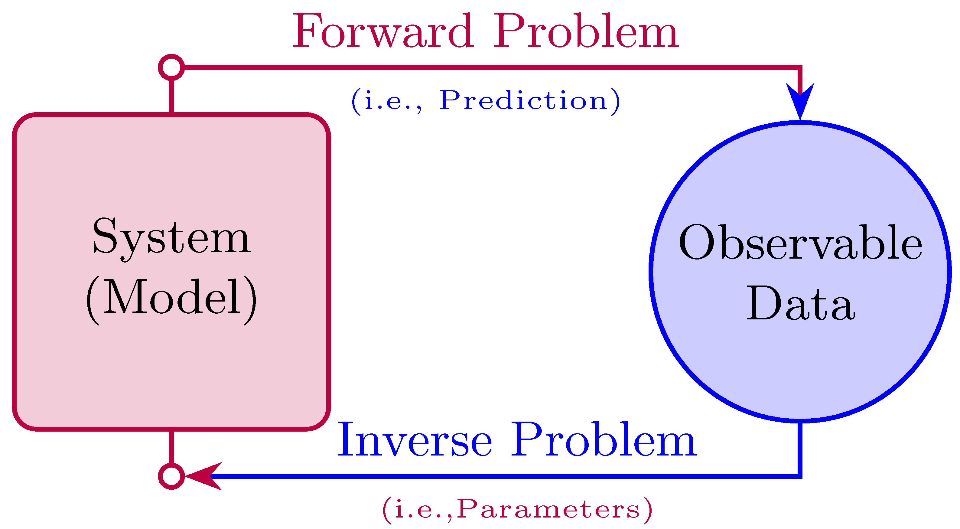
2.3. Forward and Inverse Problems

PINNs can be employed in a variety of ways [4,51]. Our primary focus here is on using PINNs to tackle both forward and inverse problems, as depicted in Figure 1.

The forward problem entails approximating solutions to ordinary or partial differential equations (DEs) by incorporating the governing physical laws into the loss function, as shown in Figure 2. It involves predicting the outcome or state of a system given known inputs and parameters. In the context of ODEs, a forward problem requires solving the differential equation to obtain the system’s response over time. For instance, in a tumor growth model, the forward problem would involve using ODEs to predict how the tumor size evolves based on initial conditions and parameters. PINNs tackle forward problems by learning to approximate the solution to these differential equations, providing insights into the system’s behavior under various conditions.

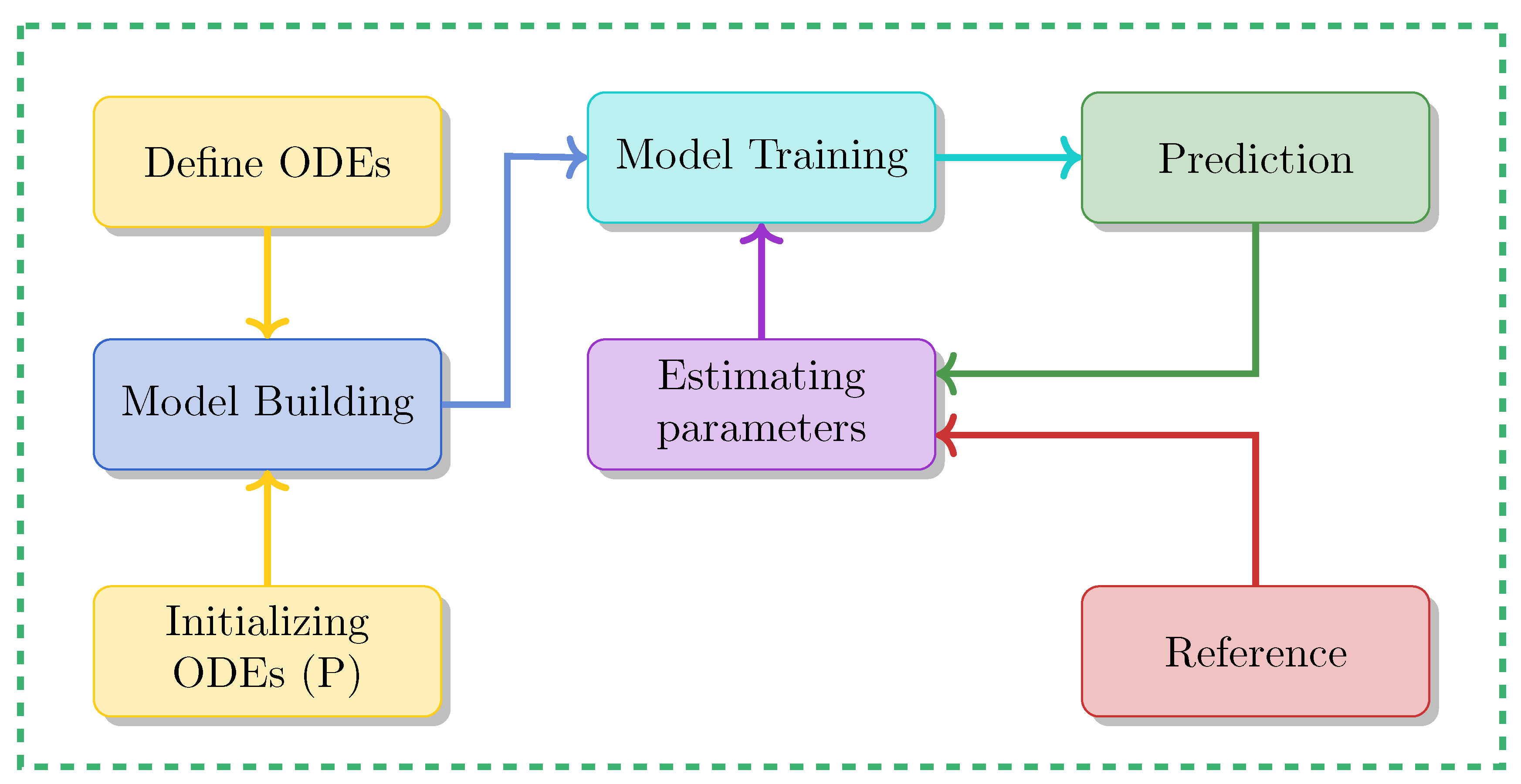
On the other hand, PINNs can also be used to solve inverse problems and estimate unknown parameters, see Figure 3. In inverse problems, the goal is to determine unknown parameters or model coefficients from observed data. This is typically achieved by incorporating physical constraints into the loss function, which quantifies the discrepancy between the model’s predictions and the observed data, while ensuring that the solutions adhere to the governing equations. This integration ensures that the estimated parameters are not only consistent with the observed data but also adhere to the underlying physical laws.

For example, in the context of a tumor growth model, an inverse problem involves estimating parameters such as the carrying capacity (K) and the cell proliferation rate ($\alpha$) from observed data (e.g., tumor size over time). During training, the PINN adjusts these parameters to minimize the difference between the model’s predicted tumor growth and the actual observed data, allowing for accurate estimation of the underlying biological dynamics.

To gain a practical understanding of PINNs, the implementations of utilized ODE-based models are outlined next sections. This hands-on approach will allow us to replicate these examples and build a foundation for applying similar techniques to related problems, which will be outlined.

3. Experimental Procedures

Utilizing PINN to tackle both forward problems and inverse problems in ODE-based dynamical systems involves several crucial steps, which can be summarized as follows:

3.1. Forward Problems

Implementing a forward solution for a dynamical system using PINNs entails several steps. These steps, detailed in Algorithm 1, can be summarized as follows:

Algorithm 1 Approximating Solution for a dynamical system Using PINNs

1: Step 1: Defining the dynamical system 2:       INPUT: System parameters and initial condition 3:       Define the differential equation: ${\displaystyle \frac{dx}{dt}}=f(x,t)$ 4: Step 2: Defining PINN Model (Network Architecture) 5:       Input: t (time or independent variable) 6:       Hidden Layers: Specify the number of hidden layers and neurons per layer. 7:       Activation Function: Choose suitable activation functions (e.g., GELU, Tanh) 8:       Output: $\widehat{x}\left(t\right)$ (state variable or dependent variable) 9: Step 3: Defining Loss Functions 10:       Data Loss: ${\mathcal{L}}_{\mathrm{Data}}={\sum }_i{|\widehat{x}\left(t_i\right)-x_i|}^2$ 11:       Physics Loss: ${\mathcal{L}}_{\mathrm{Physics}}={\left|{\displaystyle \frac{dx}{dt}}-f(x,t)\right|}^2$ 12:       Total Loss: ${\mathcal{L}}_{\mathrm{total}}={\lambda }_1·{\mathcal{L}}_{\mathrm{Data}}+{\lambda }_2·{\mathcal{L}}_{\mathrm{Physics}}$ 13: Step 4: Training PINN Model 14:       Initialize Network Parameters 15:       Use optimizer (e.g., Adam or SGD) to minimize ${\mathcal{L}}_{\mathrm{total}}$: ${\mathit{\theta }}^{*}=arg{min}_{\mathit{\theta }}{\mathcal{L}}_{\mathrm{total}}(\mathit{\theta })$ 16:       Backpropagate the loss and update the model parameters. 17:       Repeat for sufficient epochs until convergence 18: Step 5: Evaluating the Model 19:       Compare predicted $\widehat{x}\left(t\right)$ with known values, observed data, or analytical solutions if available 20:       $x\left(t\right)\approx \widehat{x}(t;{\theta }^{*})$ 21:       Plot the model predictions against the actual data or reference.

• In the first step, the differential equation that governs the dynamical system needs to be defined as detailed in Section 2.2.
• In step 2, the neural network needs to be defined, which requires specifying its architecture, including activation functions and the input range. For example, the input could be time t in the range $[0,T]$), and the output could be the approximate solution for the state variable $x\left(t\right)$, with appropriate activation functions (e.g., GELU or Tanh).
• In step 3, the loss functions are defined to guide the training process. Importantly, the total loss function consists of different parts corresponding to individual loss functions, each describing a particular aspect.
  This includes:
  • Data Loss: Measures the differences between predicted values and observed data or exact solution, expressed as

    $$\begin{array}{c}\hfill {\mathcal{L}}_{\mathrm{Data}}=\sum _i{\left|\widehat{x}\left(t_i\right)-x_i\right|}^2\end{array}$$

    (8)
  • Physics Loss: Ensures that the neural network adheres to the underlying physical law, typically formulated as a differential equation. This is achieved by computing the derivative of the network’s output with respect to its input and comparing it to the expected theoretical expression. The loss is defined as:

    $$\begin{array}{c}\hfill {\mathcal{L}}_{\mathrm{Physics}}={\left|{\displaystyle \frac{dx}{dt}}-f(x,t)\right|}^2\end{array}$$

    (9)
  The derivative ${\displaystyle \frac{d\widehat{x}}{dt}}$ is computed using PyTorch’s automatic differentiation framework. This approach allows for efficient and accurate gradient computation, enabling the enforcement of physical consistency within the training process. Finally, the total loss combines the individual loss functions:

  $${\mathcal{L}}_{\mathrm{total}}={\lambda }_1·{\mathcal{L}}_{\mathrm{Data}}+{\lambda }_2·{\mathcal{L}}_{\mathrm{Physics}}$$

  (10)

  where ${\lambda }_1$ and ${\lambda }_2$ control the trade-off between fitting the data and satisfying the physical constraints.
• In step 4, the neural network is trained. This involves initializing the network parameters, and using an optimizer like Adam or SGD to minimize the total loss over sufficient epochs until the model converges.
• In step 5, the model is evaluated. For this, one can assess the performance of the model by comparing the predicted outputs $\widehat{x}\left(t\right)$ with actual values $x\left(t\right)$ or analytical solutions, when available.

3.2. Inverse Problems

Using PINN to estimate unknown parameters from observable data, a process also known as the inverse problem, for dynamical systems described by ODEs involves several key steps, as summarized in Algorithm 2. These steps can be outlined as follows:

• Load Data: The first step involves reading timepoints t and corresponding observations x from the available sources (in our case, a CSV file containing simulated data based on the models’ ODE equations) and converting these data into numpy arrays.
• Initial Parameter Estimation: In this step, the ordinary differential equation (ODE) is defined, with $\theta$ representing the parameters to be estimated and initialized as ${\theta }_{\mathrm{init}}$. The loss function is formulated to minimize the error between the observed data and the values predicted by the model.
  In Step 3, the PINN model is defined by constructing a neural network to approximate the solution of the dynamical system governed by the ODE. The architecture of the network includes an input layer representing t (the time or independent variable), followed by hidden layers with a specified number of layers and neurons per layer (for example, two layers with 100 units each). The activation function is selected from appropriate options such as GELU or Tanh. Finally, the output layer of the network provides $\widehat{x}\left(t\right)$, the approximated state or dependent variable of the system.
  In Step 4, the model parameters, including the network parameters $\theta$ (e.g., weights, biases) and dynamical system parameters, are optimized through training. An optimizer like Adam or SGD is used to minimize the total loss ${\mathcal{L}}_{\mathrm{total}}$, adjusting both sets of parameters to reduce the error between predictions and actual values. Gradients are computed via backpropagation, and the parameters are updated accordingly. Training continues until the loss converges, signaling that the model has reached an optimal state.
  In Step 5: Evaluating the Model, the goal is to assess how well the model’s predictions match the actual data or known analytical solutions. This is achieved by comparing the predicted values $\widehat{x}(t;{\theta }^{*})$, which are the model’s outputs based on the optimized parameters ${\theta }^{*}$, to the observed values or reference data. This comparison is often visualized by plotting the predicted values against the real data, allowing for a clear inspection of how well the model fits. Additionally, the estimated parameters $\theta$ of the dynamical system are printed, providing the final values of the system’s parameters after optimization. This evaluation is important for understanding the model’s accuracy and its ability to represent the system’s dynamics.

Algorithm 2 Estimating Parameters of a dynamical system Using PINNs

1: Step 1: Load Data 2:       Read timepoints t and observations x from the available source. 3:       Convert the data to numpy arrays. 4: Step 2: Initial Parameter Estimation 5:       Define the ODE dynamical system along with its initial conditions and initial parameter values ${\theta }_{\mathrm{init}}$. 6:       Define the loss functions: ${\mathcal{L}}_{\mathrm{total}}={\lambda }_1·{\mathcal{L}}_{\mathrm{Data}}+{\lambda }_2·{\mathcal{L}}_{\mathrm{Physics}}$. 7: Step 3: Defining PINN Model (Network Architecture) 8:       Input: t (time or independent variable) 9:       Hidden Layers: Specify the number of hidden layers and neurons per layer. 10:       Activation Function: Choose suitable activation functions (e.g., GELU, Tanh) 11:       Output: $\widehat{x}\left(t\right)$ (state variable or dependent variable) 12:       Specify the parameters $\theta$ to be estimated as trainable parameters. 13: Step 4: Training PINN Model 14:       Initialize Network Parameters 15:       Use optimizer (e.g., Adam or SGD) to minimize ${\mathcal{L}}_{\mathrm{total}}$: ${\mathit{\theta }}^{*}=arg{min}_{\mathit{\theta }}{\mathcal{L}}_{\mathrm{total}}(\mathit{\theta })$ 16:       Backpropagate the loss and update the NN and dynamical system parameters. 17:       Repeat for sufficient epochs until convergence 18: Step 5: Evaluating the Model 19:       Compare predicted $\widehat{x}\left(t\right)$ with known values, observed data, or analytical solutions if available 20:       $x\left(t\right)\approx \widehat{x}(t;{\theta }^{*})$ 21:       Plot the model predictions against the actual data or reference. 22:       Print the estimated parameters $\theta$ of the dynamical system.

4. Results

In order to make our study reproducible, we start our analysis by providing information about parameter settings. Selecting the appropriate hyperparameters is crucial to optimizing a neural network’s performance. The number of hidden layers affects the model’s depth; while additional layers enable the model to learn more complex patterns, they also increase the risk of overfitting if the network is excessively deep. Based on experiments with 2, 3, and 4 layers, the optimal number was selected to balance complexity and overfitting, as outlined in

Table 1. Parameters settings for the models Tumor Growth (TG), Gene Expression (GE), and the SIR (Susceptible, Infected, Recovered).

	TG	GE	SIR
INPUT_DIM	1	1	1
HIDDEN LAYERs	3	2	3
HIDDEN_DIMS	64	64	100
OUTPUT_DIM	1	2	3
ACTIVATION_FN	$GELU$	$GELU$	$Tanh$
LEARNING RATE	× ${10}^{-3}$	× ${10}^{-3}$	× ${10}^{-3}$
STATE VARIABLES	$X\left(0\right)=1$	$M\left(0\right)=1$, $P\left(0\right)=1$	$S\left(0\right)=0.99$, $I\left(0\right)=0.01$, $R\left(0\right)=0.0$
PARAMS	$\alpha =0.3,K=100$	$PN=50,K_m=0.7,{\gamma }_m=0.8,$	$\beta =0.5,\gamma =0.05$
		$k_p=0.6,{\gamma }_p=0.6$
SIMULATION TIME	50	50	100
NUM_SAMPLES	120	100	120
BATCH_SIZE	32	32	32
EPOCHS	1000	3000	4000
EPOCH_INTERVAL	200	250	50
PATIENCE	100	200	50

. Hidden dimensions denote the number of neurons in each layer. Larger dimensions allow the model to capture more features but can also lead to overfitting and higher computational costs as well. After trying different values, the chosen dimension aimed to strike a balance between model capacity and efficiency. Activation functions introduce non-linearity into the model. Our experiments with PINNs showed that functions such as $ReLU$, $Tanh$, and $GELU$ outperformed $Sigmoid$, likely due to their effectiveness in addressing vanishing gradient issues. These activation functions contributed to better convergence and stability. The Learning Rate governs the step size during optimization. After testing values of 1 × ${10}^{-2}$, 1 × ${10}^{-3}$, and × ${10}^{-4}$, it was observed that a rate of × ${10}^{-2}$ might have caused rapid convergence or oscillation, while × ${10}^{-4}$ led to slower convergence. The selected value (× ${10}^{-3}$) balanced fast learning with stable convergence. Epochs determine how frequently the model reviews the entire dataset, and Patience helps to stop training early if performance stagnates. The selected values balance comprehensive learning with the prevention of overfitting or excessive training.

In our implementation, the total loss function is defined as in Equation (10), where the weighting parameters ${\lambda }_1$ and ${\lambda }_2$ control the trade-off between fitting observed data and enforcing physical laws. These values were determined through empirical tuning: ${\lambda }_1$ was selected to prioritize data accuracy without overfitting, while ${\lambda }_2$ was gradually adjusted to ensure the model accurately captured physical behavior without dominating the loss function. Both parameters were constrained to the range $[0,1]$. The best performance was achieved with ${\lambda }_1=0.7$ and ${\lambda }_2=0.3$. Deviations from this configuration, whether by setting the weights too low or too high, led to an imbalance, resulting in either weak enforcement of physical principles (particularly affecting the estimated parameter values) or diminished data accuracy (i.e., suboptimal data fitting), respectively.

Table 1 gives a summary of three models studied in the following: Tumor Growth (TG), Gene Expression (GE), and an Epidemiological system (ES), the SIR (Susceptible, Infected, Recovered) model. Each model receives a single input, as indicated by the input dimension (INPUT_DIM) set to 1 across all models. The model architectures differ slightly, with the GE having two hidden layers, while the TG and SIR models are deeper, with three hidden layers. The number of neurons per hidden layer, known as HIDDEN_DIMS, is 100 for both the TG and SIR models, while the GE model uses 64 neurons, reflecting the computational complexity and capacity tailored to each model’s needs.

The output dimensions (OUTPUT_DIM) differ as well, with the TG model producing a single output, the GE model producing two, and the SIR model generating three outputs, corresponding to the three states in the SIR model. The activation functions used also vary; TG and GE models utilize the GELU activation function, known for its smooth, non-linear properties, while the SIR model employs the Tanh function, suited for modeling smooth transitions between states.

The learning rate, a critical hyperparameter controlling the step size during model optimization, is consistently set to × ${10}^{-3}$ for all models. Initial conditions, or state variables, are specified uniquely for each model, such as the initial population states for the SIR model (S, I, R) and specific starting levels for the TG and GE models. Each model also has unique parameters tailored to its dynamics, such as growth rates and carrying capacities, which are crucial for simulating realistic scenarios.

The simulated data is produced using the models’ ODE equations. The time range for simulation differs slightly, with the TG and GE models running for 50 time units, while the SIR model extends to 100. The number of samples used in training is 120 for the TG and SIR models and 100 for the GE model. The generated data (NUM_SAMPLES) is divided into training and testing sets, with $80\%$ allocated for training and $20\%$ reserved for testing. Here, “training sample” and “test samples” correspond to the true/exact solution. All models are trained with a batch size of 32, meaning that 32 samples are processed before updating the model’s parameters.

Training epochs, the number of complete passes through the training data, is set at 1000 for the TG model, 3000 for GE model, and 4000 for the SIR model, likely reflecting the greater complexity or longer convergence time needed for the SIR model. Evaluations are made across all models at every EPOCH_INTERVAL epoch, as specified by the EPOCH_INTERVAL. The patience parameter, set to 100 for TG, 200 for GE, and 50 for SIR model, specifies the number of epochs allowed without improvement before early stopping is triggered, preventing overfitting and unnecessary computation.

The same settings were used for both predicting the forward solution and for parameter estimation, with one exception: the number of epochs during parameter estimation differed. It was set to 2000 for the TG model, 15,000 for the GE model, and 10,000 for the SIR model. This variation is due to slight differences in the models and training functions used for each problem (forward vs. inverse). For example, in the inverse problem, the model requires initial values for the parameter being estimated, whereas this is not needed in the forward problem.

In the parameter estimation process, values for STATE VARIABLES and SIMULATION TIME were not provided as predefined inputs but had to be extracted from the generated data. The initial parameter values were as follows: for TG, $\alpha$ and K were set to [$1.0,10.0$]; for GE, $k_m$, $k_p$, ${\gamma }_p$, and ${\gamma }_m$ were all set to 1; and for SIR, $\alpha$ and $\gamma$ were both set to 1.

Overall, these configurations demonstrate how the models are precisely calibrated to fulfill their respective tasks, balancing complexity, computational efficiency, and the necessity for accurate simulation and prediction.

4.1. Tumor Growth Model

The first model, we analyze is the tumor growth model (TGM) (see Methods section for details). For the TGM, we use a Physics-Informed Neural Network (PINN) to model cancer progression dynamics using the differential Equation (2), which describes the rate at which tumor size changes over time.

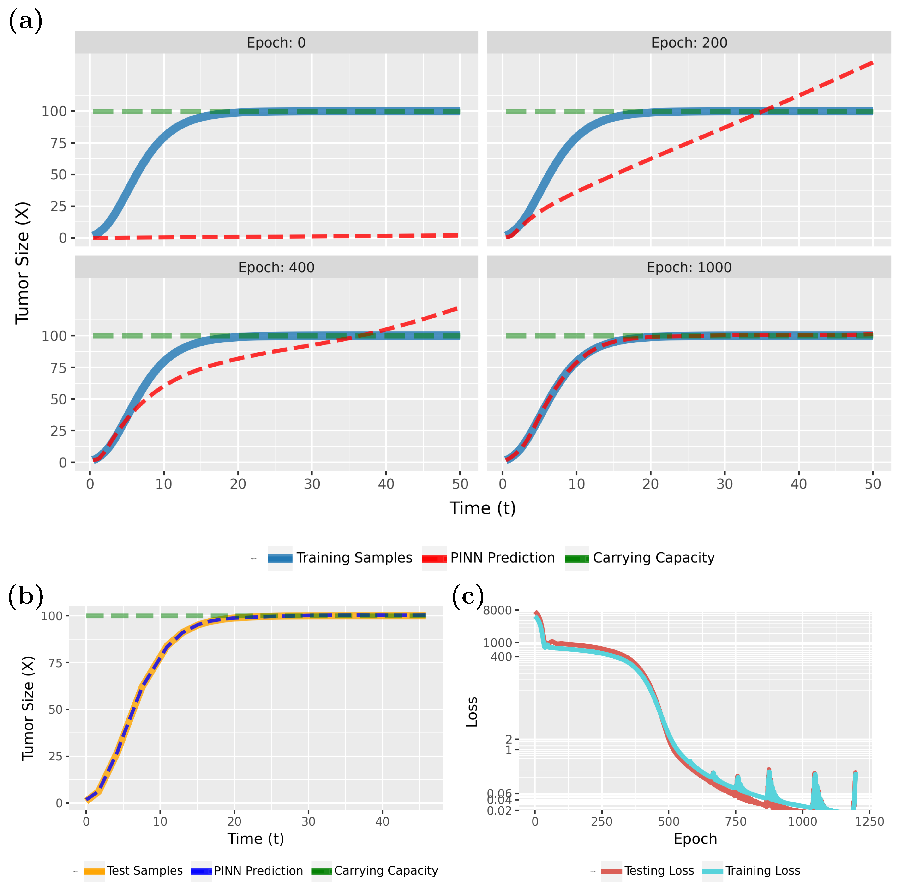
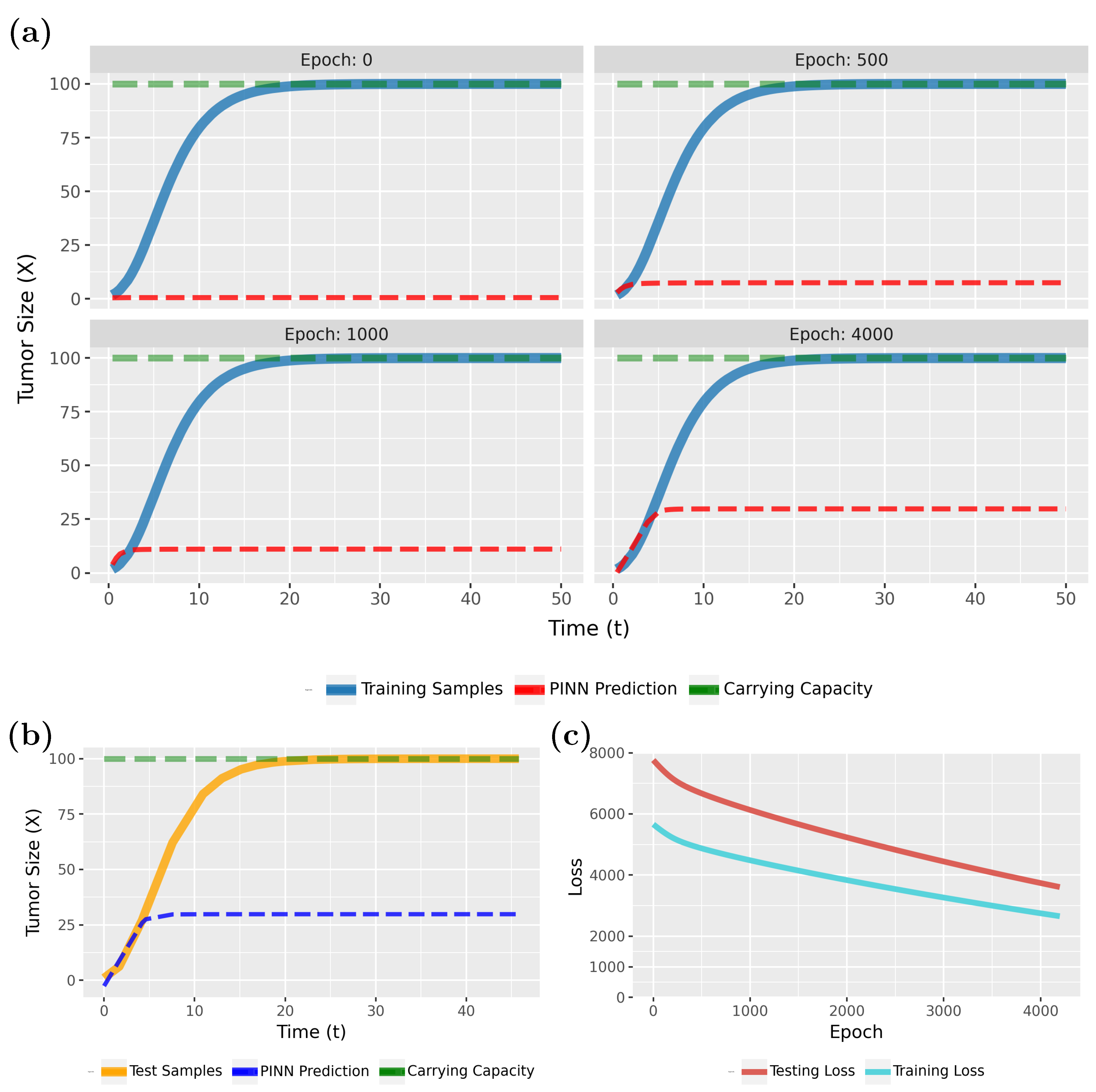
Figure 4 compares the PINN predictions (in red) with the actual tumor growth (in blue) modeled by Equation (2). Specifically, in Figure 4a (epoch 0), the initial results are shown, whereas the following three subfigures show the effects of the training for 200, 400, and 1000 epochs. From this one can see that the model rapidly converges to a true model. This is also confirmed by the loss function, shown in Figure 4c.

Notably, the PINN continues to improve for up to 500 epochs before stabilizing. As the loss values approach near-zero, we attempted to highlight this variation by adjusting the Y-axis scale. However, utilizing the early stopping technique, with the patience parameter specified in Table 1, training will halt if no further improvement in loss accuracy is detected. In this case, early stopping occurred at epoch 1033.

To see that the PINN can generalize to new sample points, we show in Figure 4b results for test data for the converged model. Overall, these results are very similar to Figure 4a (epoch 1000) and indicate excellent generalization capabilities. Overall, our findings show that PINNs could accurately approximate tumor growth curves even from sparse data (see Table 1; a total of 120 samples were used, with $80\%$ allocated for training and $20\%$ for testing), with the predicted patterns closely aligning with the true model.

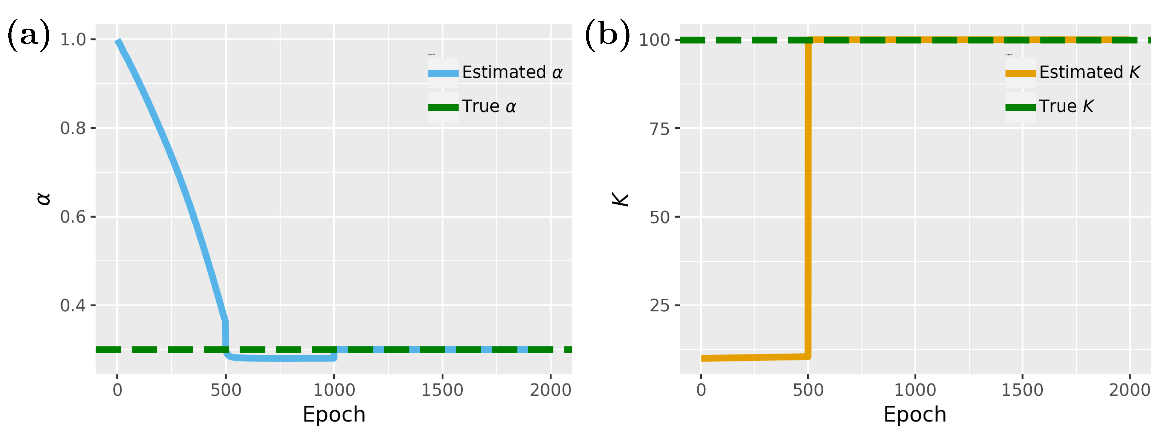
In Figure 5, we show results for the inverse problem, whereas Figure 5a shows results for the proliferation rate $\alpha$ and Figure 5b for the carrying capacity K. For the carrying capacity K one can see that convergence is achieved for about 500 epochs, while for the proliferation rate $\alpha$, 1000 epochs are needed. Interestingly, between 500 and 1000 epochs the model is stuck in local minima close to the optimal value of $\alpha$ but eventually finds the optimal solution.

4.2. Fine Tuning of Hyperparameters

To illustrate how the effectiveness of PINNs relies on the careful fine tuning of the neural network architecture and hyperparameters, as well as the importance of customized configurations tailored to specific system dynamics, we discuss some details of the implementation steps outlined in Section 3 and the fine-tuning considerations discussed in Section 4. For this, we train the PINN model for the TGM as outlined in Table 1, with some modifications to emphasize the impact of hyperparameter tuning on the model’s learnability and performance. Specifically, we reduced the number of hidden layers from three to two, with 32 neurons per layer (instead of 64). Additionally, the learning rate was set to (1 × ${10}^{-4}$), and the $Sigmoid$ activation function was used.

As shown in Figure 6a,b, for the training and testing sets, the model performs poorly, failing to approximate the solution even after 4000 epochs. The loss accuracy, shown in Figure 6c, further highlights the model’s poor performance under this configuration. This underscores the critical importance of hyperparameter selection for achieving efficient performance with fewer computational steps. Conversely, using the same configuration from Table 1, the model was able to approximate the solution perfectly within just 1000 epochs, as shown in Figure 4. Overall, this demonstrates the sensitivity of the performance of PINNs to moderate changes in the network design and training parameters.

4.3. Gene Expression Model

The next model for which we illustrate the application of PINNs is a gene expression model (see Methods section for details). This model simulates the regulation of gene activity using a system of ordinary differential equations, as shown in Equations (3) and (4). These equations incorporate various biological interactions and regulatory mechanisms.

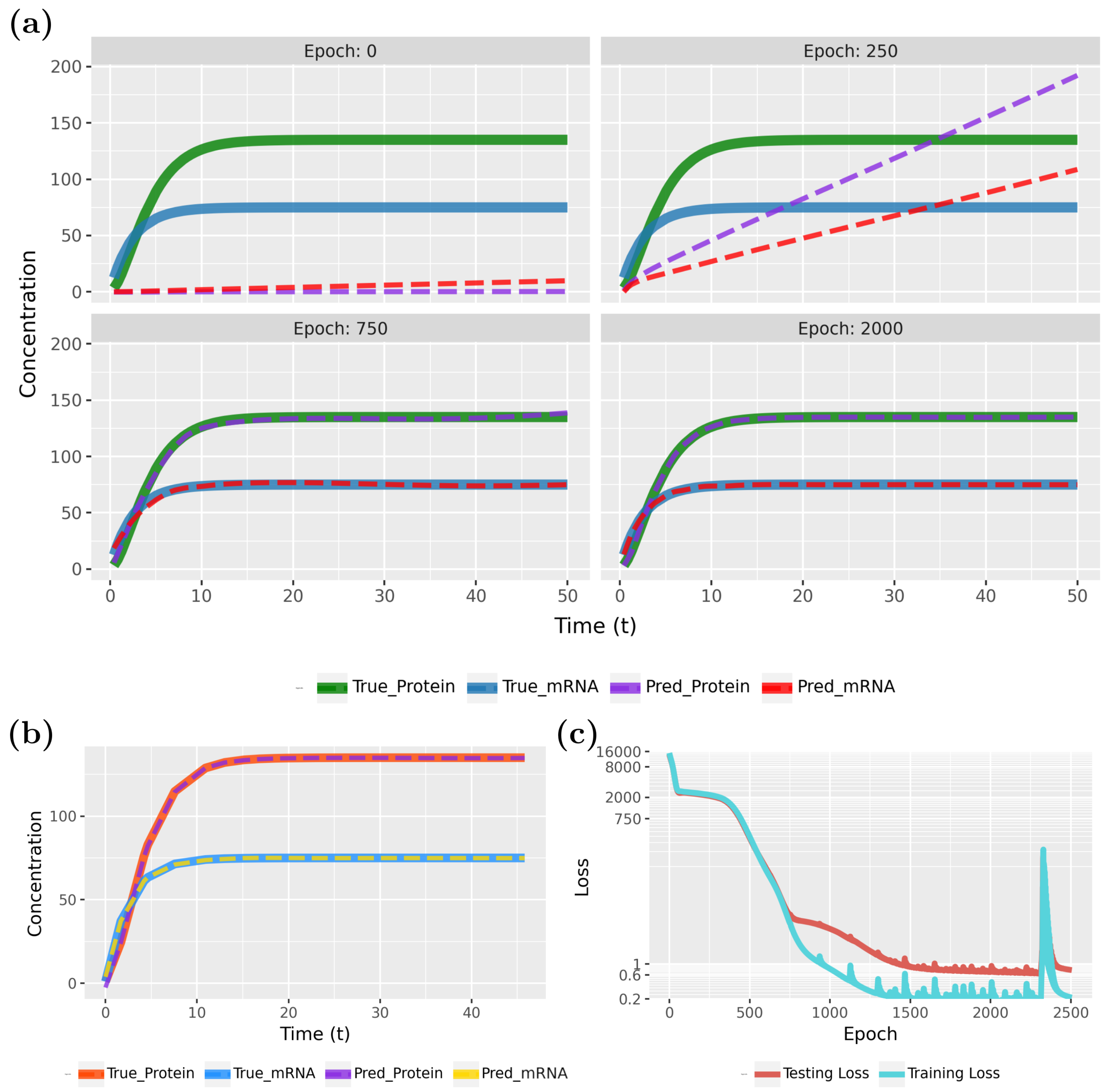
Figure 7 compares the PINN predictions with the actual synthesis and degradation of mRNAs and proteins. Specifically, in Figure 7a (epoch 0), results for the initialization are shown, whereas the following three subfigures show the effects of the training for 250, 750, and 2000 epochs. From the behavior of the curves, one can see that the model rapidly converges to true model.

The convergence of the model is also confirmed by the loss function, shown in Figure 7c. Notably, the PINN continues to improve for up to 800 epochs before stabilizing. As the loss values approach near-zero, we attempted to highlight this variation by adjusting the Y-axis scale. However, utilizing the early stopping technique, with the parameters specified in Table 1, training will halt if no further improvement in loss accuracy is detected. In this case, early stopping occurred at epoch 2506.

To demonstrate the PINN’s ability to generalize to new sample points, we present the test data results for the converged model in Figure 7b. These results highlight the model’s generalization capabilities. Our findings indicate that PINNs can accurately approximate gene expression dynamics, including mRNA and protein synthesis and degradation within a cell, even with sparse data. Specifically, we used a total of 100 samples, with $80\%$ allocated for training and $20\%$ for testing (see Table 1), and observed that the predicted patterns closely align with the true model. 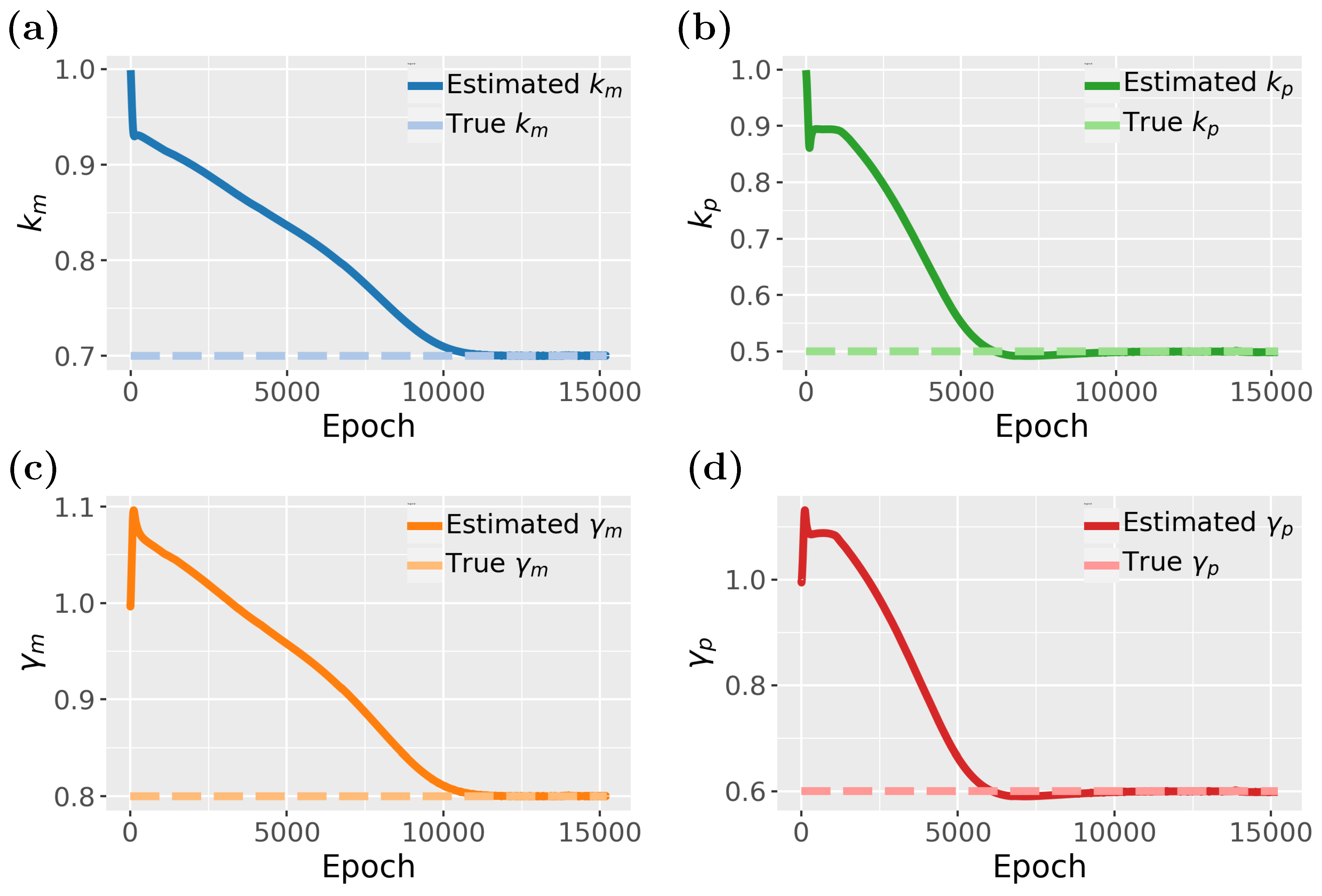Figure 8 illustrates the estimated parameters associated with gene regulation, such as $k_m$, $k_p$, ${\gamma }_m$, and ${\gamma }_p$, and their influence on expression levels.

In Figure 8, we study the inverse problem of the gene expression model. In total, the model consists of four parameters $k_m,k_p,{\gamma }_m,{\gamma }_p$ that need to be estimated. From Figure 8, it seems that $k_p$ and ${\gamma }_p$ converges much faster than $k_m$ and ${\gamma }_m$, however, when looking carefully one notices a slight dip between 5000 and 10,000 epochs. Hence, all four parameters converge around 10,000 epochs but $k_p$ and ${\gamma }_p$ are, for a time, stuck in local maxima close to the true value before reaching the optimal values. Overall, the results demonstrate that the PINN effectively captures the dynamics of gene expression and also allows the estimation of its parameters.

4.4. SIR Model

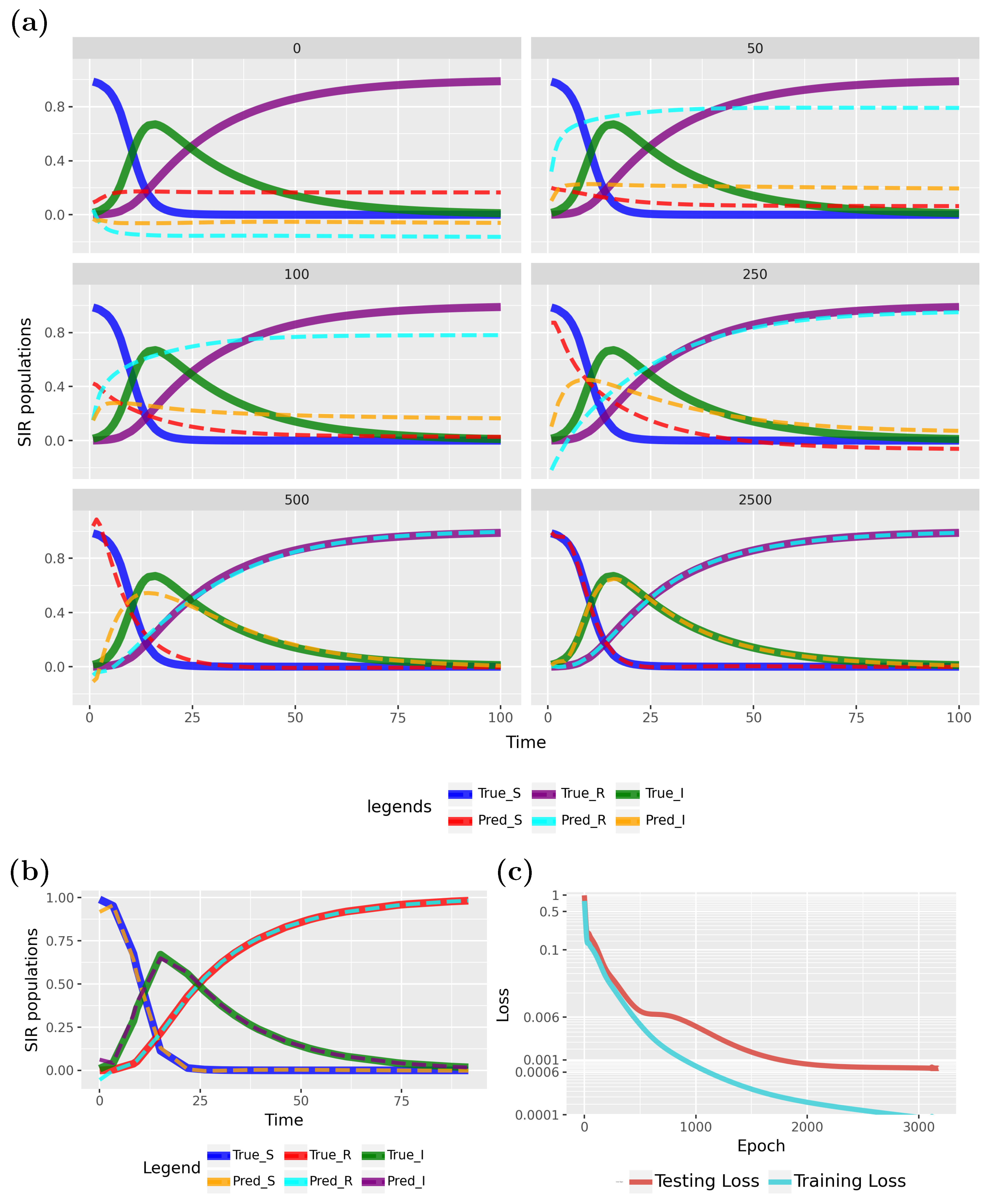
The last model we study is the SIR (Susceptible, Infected, Recovered) model from epidemiology (see Methods section for details). The SIR model describes the spread of an infectious disease using a system of ordinary differential equations (ODEs), shown in Equations (5)–(7). Figure 9 presents a comparison between PINN predictions and the true model.

Specifically, Figure 9a shows results from epoch 0 (initialization), while the subsequent five subfigures illustrate the effects of training at epochs 50, 100, 250, 500, and 2500. The model converges rapidly to the true data, as indicated by the loss function in Figure 9c. The PINN continues to improve up to approximately 2000 epochs before stabilizing. To better highlight variations at near-zero loss values, the Y-axis was scaled. Early stopping, as detailed in Table 1, was employed to halt training when no further loss improvement was observed, which occurred at epoch 3175.

To show the generalization ability of the PINN, we show test data results for the converged model in Figure 9b. These results underscore the model’s strong generalization capabilities. This demonstrates that a PINN can effectively estimate transmission and recovery rates, with forecasts closely aligning with the true model. Specifically, we used 120 samples, with $80\%$ for training and $20\%$ for testing (see Table 1), and the predicted patterns closely matched the true model.

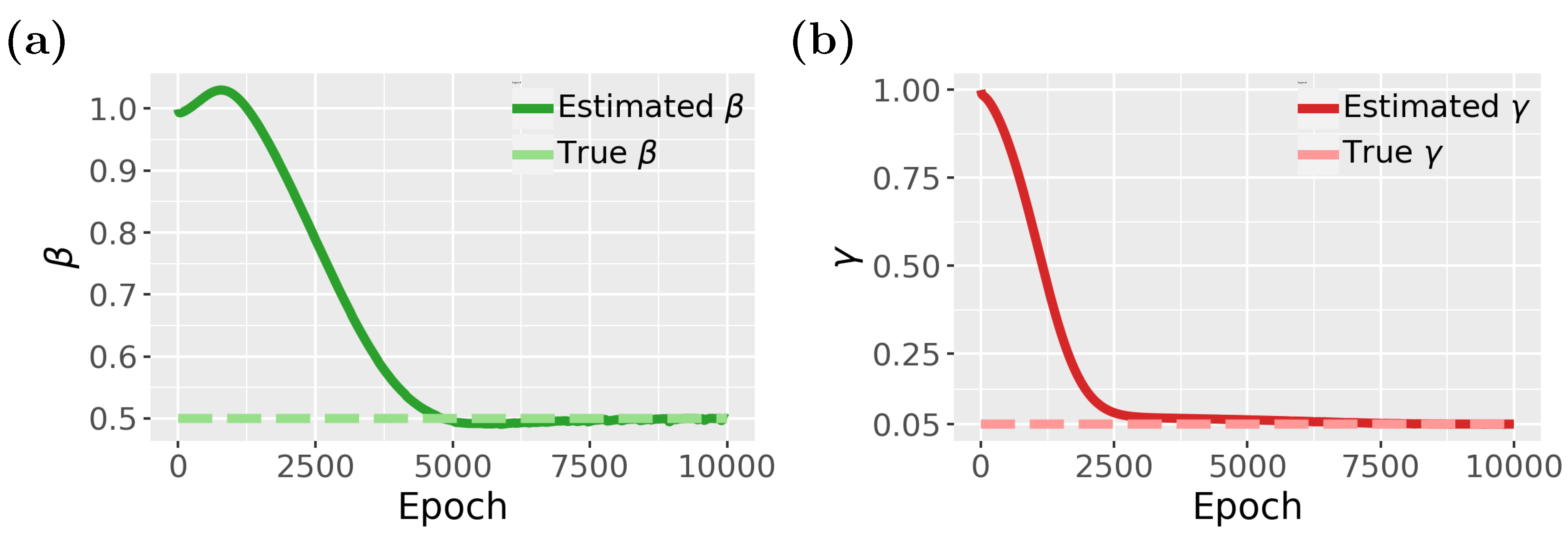
Finally, in Figure 10, we show results for the inverse problem for the SIR model, where we estimate the two parameters, $\beta$ and $\gamma$. As one can see from Figure 10a,b, both parameters converge to the true parameter values, however, again, only after escaping from local minima (see epochs 5000 to 7500 for $\beta$ and epochs 2500 to 7000 for $\gamma$).

5. Code Availability

To allow the reproduction of our results focusing on systems of ordinary differential equations, we created a Python package called ODE-PINN. The libraries used in our code provide essential functionalities for studying forward and inverse problems for a large variety of systems of ordinary differential equations.

We employ scipy.integrate.odeint to solve ordinary differential equations, while numpy and pandas are used for numerical computations and data handling. To split data into training and testing sets, we use train_test_split from sklearn.model_selection. Our deep learning models are built with PyTorch, utilizing torch as the framework for neural networks. For efficient data loading and batching, we rely on DataLoader and TensorDataset from torch.utils.data. Network architectures are defined using torch.nn, and training optimization via torch.optim. We apply xavier_uniform_ from torch.nn.init for weight initialization, and autograd.grad from torch.autograd to compute gradients of outputs with respect to inputs, which is essential for enforcing physics-informed loss functions during training. The scipy.optimize.minimize function is also used to solve optimization problems, particularly useful for fine-tuning model parameters or minimizing error metrics in inverse problems. Finally, plotnine is used to visualize data and results. The complete code and associated datasets for this manuscript are available on GitHub at https://github.com/AmerFarea/ODE-PINN (accessed on 10 May 2025).

6. Discussion

This paper investigates the use of PINNs for modeling dynamical systems governed by systems of ODEs, revealing its substantial effectiveness and versatility. Our case studies—tumor growth, gene expression, and disease spread using the SIR model—demonstrate the abilities of a PINN to accurately approximate solutions and estimate parameters with notable precision.

The application of PINNs across these diverse systems underscores their versatility and strength. They excel at integrating physical constraints with observational data, delivering accurate and physically consistent solutions. This is particularly advantageous for complex systems where other methods might struggle.

However, the effectiveness of PINNs is influenced by the sensitivity of network architecture and hyperparameters, which necessitates careful tuning for optimal performance. Challenges such as handling noisy and sparse data, and addressing inverse problems highlight the need for robust regularization techniques and improved methods for parameter estimation.

The detailed configuration, as outlined in the Section 4 section, provides insights into the experimental setups and performance of PINNs across various models. The table outlines key parameters such as network architecture, activation functions, learning rates, and simulation details. For example, the tumor growth model was designed with three hidden layers, each having 64 units, and utilized GELU activation functions. The gene expression model had a similar setup but with two hidden layers, also using GELU activation. In contrast, the SIR model featured a network with three hidden layers of 100 units each and employed Tanh activation functions.

The variations in architecture and parameters highlight the importance of tailoring PINN configurations to the specific characteristics of the dynamical system being modeled. For example, the different activation functions (GELU vs. Tanh) and the adjustments in the number of hidden layers reflect attempts to optimize model performance for diverse types of data and system dynamics. The learning rates and batch sizes were consistent across models, emphasizing a common approach to training stability, though the number of epochs and patience settings varied, suggesting different convergence criteria and training durations tailored to each model’s complexity.

These parameter settings underscore the adaptability of PINNs but also point to the sensitivity of their performance to hyperparameters and network design. Careful tuning is essential to achieve optimal results, as shown by the varying results across the different case studies. This highlights both the robustness and the challenges associated with applying PINNs to diverse dynamical systems.

Our results demonstrate that PINNs for systems of ordinary differential equations (ODEs) can effectively model biological mechanisms, systems biology, and epidemiological processes. This is important to highlight because, so far, the primary focus of PINNs has been on partial differential equations (PDEs) for physics-related problems. In contrast, fields outside of physics have been largely understudied. Since ODEs dominate in these fields, we concentrated our study on such dynamical systems to showcase their application.

From a technical standpoint, PDEs differ significantly from ODEs, and consequently, the resulting PINNs also differ. To facilitate the use of ODE-based PINNs, we provide a Python software implementation to complement our presentation. We believe that such applications hold tremendous potential for addressing medical and economic problems, many of which are yet to be explored.

7. Conclusions

This paper explores the application of Physics-Informed Neural Networks (PINNs) for modeling dynamical systems described by ordinary differential equations (ODEs), with a focus on biological and epidemiological domains that have received relatively little attention in the PINN literature. We present three detailed case studies—tumor growth, gene expression, and disease spread using the SIR model—demonstrating how PINNs can be effectively used for both forward problem approximation and parameter estimation from synthetic data.

Beyond demonstrating the practical applicability of PINNs in these new contexts, our study also emphasizes important implementation aspects. We show that the performance of PINNs is highly sensitive to the choice of network architecture and training strategy, underscoring the need for problem-specific design and tuning. These insights are valuable for researchers and practitioners aiming to apply PINNs to other real-world systems. In addition to these applied contributions, the paper serves a practical purpose by providing clear examples, structured explanations, and an openly accessible Python library—ODE-PINN—that enables the reproduction and extension of our results. This positions the work as both a practical demonstration of PINNs in non-traditional domains and a valuable resource for newcomers to the field.

In summary, this study showcases the potential of PINNs for modeling ODE-based systems in biology and epidemiology, emphasizing their role in improving our understanding and management of dynamic systems. By offering practical tools and case studies, we provide resources for further exploration in research.