Population Median Estimation Using Auxiliary Variables: A Simulation Study with Real Data Across Sample Sizes and Parameters

Abstract

This paper introduces an enhanced class of ratio estimators, which employ the transformation technique on an auxiliary variable under simple random sampling to estimate the population median. The transformation strategy can reduce both the bias and mean square error, which can help estimators become more efficient. The bias and mean square error of proposed estimators are investigated up to the first order of approximation. Through simulation studies and the analysis of various data sets, the performance of the proposed estimators is compared to existing methods. The proposed class of estimators improves the precision and efficiency of median estimation, ensuring more accurate and dependable results in various practical scenarios. The findings reveal that the new estimators show superior performance under the given conditions compared to traditional estimators.

1. Introduction

The use of auxiliary information is necessary for improving estimator efficiency in survey sampling, both in the planning and estimation stages as well. The median is frequently a more suitable measure of central tendency than the mean when dealing with variables that show highly skewed distributions, such as income, expenditure, taxation, consumption, and production. For researchers who want to identify the exact center of their data, the median is an essential tool because these variables regularly show higher skewness. However, the study of efficient techniques for precisely estimating medians in finite populations is still comparatively less focused, despite the extensive literature on the estimation of means, variances, proportions, regression coefficients, and totals. The gap emphasizes the need for more study to enhance methods that can use auxiliary data to estimate the median more accurately. For more details, we refer to [1,2].

In many situations, the median plays an important role in analyzing skewed data or outliers. It improves statistical accuracy by reflecting survey answers in the social sciences, income in economics, pollutant levels in environmental research, patient outcomes in health, and real estate market patterns. The estimation of the median under simple random sampling was initially examined by [3,4,5,6], and they investigated how to calculate it using auxiliary information. Following the work of [6], several estimators have been developed for population median calculation using the different sampling methods. Certain unique methods for enhancing ratios and regression estimators for the median were suggested by [7]. Using double sampling methods, [8] introduced some methods to discuss median estimation. An improved family of estimators using two auxiliary variables in double sampling to estimate the population median was obtained by [9]. The minimum unbiased estimator, using the known median of the auxiliary variable, was proposed by [10]. Later on, improvements in the accuracy of median estimation by using two auxiliary variables under the two-phase sampling technique was discussed by [11]. Some improved types of estimators to estimate the population median under simple random and stratified random sampling were obtained by [12,13]. Under different sampling methods, by utilizing the auxiliary information for different population parameters, some new types of estimators were obtained by [14,15]. While this study focuses on robust median estimation in survey sampling, we acknowledge classical approaches such as least squares estimation (LSE) and multi-innovation least squares (MILS) methods, which are widely used in parameter estimation and model fitting under noisy conditions [16]. In recent years, many researchers are focusing on introducing the new efficient estimators to estimate the population median under different sampling methods. For more details about median estimation, we refer to [17,18,19,20,21,22,23,24,25], and references therein.

The median is less affected by outliers than the mean and is better suited for skewed data sets. It provides a more precise representation of typical values, as it is not influenced by extreme values. The reliability of this measure is enhanced in environmental studies and surveys, where results may be affected by fluctuating significant increases or extreme responses. Motivated by [26,27], this paper introduces an enhanced class of ratio estimators, which employ the transformation techniques as an auxiliary variable in simple random sampling to estimate the population median. The use of transformation methods can help minimize both the bias and mean square error, leading to more efficient estimators. Below are some important aspects of the newly proposed class of estimators for practical applications:

• These improved estimators reduce bias and MSE, making median estimates more accurate and reliable. Our estimators use unique transformation techniques that include the inter-quartile range, mid-range, quartile average, quartile deviation, and robust measures (trimean and decile mean) on auxiliary variables to improve precision. This helps estimators handle data variability and enhance efficiency.
• The suggested estimators are flexible to skewed distributions and data sets with outliers, in contrast to many other estimators previously in use. Because of their flexibility, they are especially useful in domains such as environmental research, healthcare, and income analysis.
• The suggested estimators perform well with simple random sampling, which is one of the most often used sampling methods in survey research. Their usefulness across multiple areas can be improved by adapting them to diverse data distributions. This practical applicability makes them valuable tools for policymakers, researchers, and industry professionals.
• By considering additional data characteristics, such as the relationships between the target and auxiliary variable, the new estimators enhance their effectiveness in more complex survey designs, while filling a gap in the existing statistical literature. This contribution not only advances practical applications but also paves the way for future developments in the field.

Limitations of existing estimators: Traditional median estimators often perform poorly when the data are skewed or contains outliers, which is common in practical fields such as income analysis, healthcare, and environmental studies. These estimators typically rely on conventional measures that are sensitive to extreme values.

Motivation for robust transformations: To address these limitations, we introduce a new class of estimators that incorporate robust and non-conventional measures (e.g., interquartile range, trimean, quartile deviation, decile mean) through transformation techniques. These measures enhance stability and efficiency by reducing sensitivity to skewness and outliers.

Improvement in efficiency: The motivation is also grounded in improving estimator performance in terms of the bias and mean squared error (MSE). The proposed transformation-based estimators consistently demonstrate higher percent relative efficiency (PRE) in both simulated and real-world data sets, as shown in our analysis.

The structure of this paper is organized as follows: Section 2 provides a thorough explanation of the methods and notations utilized in this study. A review of existing estimators is outlined in Section 3. The proposed class of estimators is introduced and examined in detail in Section 4. Section 5 presents a rigorous mathematical comparison of these estimators. To validate the theoretical findings from Section 5, a simulation study is conducted in Section 6, where five different artificial populations are generated using various probability distributions. Additionally, this section includes numerical examples to illustrate the practical implementation of the theoretical results. Finally, Section 7 discusses the key results and provides potential directions for future research.

2. Variables and Notation

Suppose the auxiliary variable is denoted by X and the study variable by Y for a finite population consisting of N units, denoted as $\Gamma =({\Gamma }_1,{\Gamma }_2,\dots ,{\Gamma }_N)$. For each unit i where $i=1,2,\dots ,N$, the corresponding values of the auxiliary and study variables are $x_i$ and $y_i$, respectively. Let a random sample of size n be selected from the population of size N with the condition that $n<N$ under simple random sampling without replacement (SRSWOR). The population medians for the study and auxiliary variables are represented as $M_y$ and $M_x$, and the sample medians as $\widehat{M_y}$ and $\widehat{M_x}$. Let $C_{M_y}$ and $C_{M_x}$ represent the population coefficients of variation of the study variable Y and the auxiliary variable X, respectively. The associated probability density functions for the population medians are $f_y\left(M_y\right)$ and $f_x\left(M_x\right)$. The correlation coefficient between $M_y$ and $M_x$ is denoted by ${\rho }_{yx}$ and is defined as $\rho (M_y,M_x)=4P_{11}(y,x)-1,$ where $P_{11}=P(y\le M_y\cap x\le M_x).$

To determine the mathematical properties of different estimators, the relative error terms are utilized as follows:

$$e_0=\left({\displaystyle \frac{{\widehat{M}}_y-M_y}{M_y}}\right)$$

and

$$e_1=\left({\displaystyle \frac{{\widehat{M}}_x-M_x}{M_x}}\right),$$

such that $E\left(e_i\right)=0$ for $i=0,1$.

$$E\left(e_0^2\right)=\delta C_{M_y}^2,$$

$$E\left(e_1^2\right)=\delta C_{M_x}^2,$$

$$E\left(e_0{e}_1\right)=\delta C_{M_{yx}}={\rho }_{yx}{C}_{M_y}{C}_{M_x},$$

where

$$C_{M_y}={\displaystyle \frac{1}{M_y{f}_y\left(M_y\right)}},$$

$$C_{M_x}={\displaystyle \frac{1}{M_y{f}_x\left(M_x\right)}},$$

denote the population coefficient of variations of the study variable Y and the auxiliary variable X, and

$$\delta ={\displaystyle \frac{1}{4}}\left({\displaystyle \frac{1}{n}}-{\displaystyle \frac{1}{N}}\right),$$

is the finite population correction factor.

3. Previously Proposed Estimators

This section explores the biases and mean squared errors associated with existing estimators used for estimating the finite population median. We then compare these results with those of our new estimators to identify potential improvements.

The unbiased common estimator for calculating the population median is the median per unit estimator proposed by [3] and is stated as follows:

$${\widehat{M}}_{GR}={\widehat{M}}_y.$$

(1)

The variance of ${\widehat{M}}_{GR}$ is given by

$$Var\left({\widehat{M}}_y\right)=\delta M_y^2{C}_{M_y}^2,$$

(2)

where $\delta$ and $C_{M_y}$ are defined in Section 2.

This estimator, called the median per unit estimator, uses the sample median to estimate the population median under simple random sampling. It serves as a baseline method due to its simplicity and unbiasedness, but it may be less efficient than other estimators that use auxiliary information. Several authors have proposed alternative estimators that utilize auxiliary information to improve efficiency. Examples of such estimators are presented starting from Equation (3) onward.

A ratio estimator for the median obtained by [6] is defined as

$${\widehat{M}}_R=\left({\displaystyle \frac{{\widehat{M}}_y}{{\widehat{M}}_x}}\right)M_x.$$

(3)

The following formulas are used to express the bias and MSE of ${\widehat{M}}_R$:

$$Bias\left({\widehat{M}}_R\right)\cong \delta M_y\left(C_{M_x}^2-C_{M_{yx}}\right)$$

(4)

and

$$MSE\left({\widehat{M}}_R\right)\cong \delta M_y^2\left(C_{M_y}^2+C_{M_x}^2-2C_{M_{yx}}\right).$$

(5)

The difference estimator for ${\widehat{M}}_D$ introduced by [10], which is defined as

$${\widehat{M}}_D={\widehat{M}}_y+d\left(M_x-{\widehat{M}}_x\right),$$

(6)

where d is an unknown constant, and the optimum values of the d is given below:

$$d_{opt}={\displaystyle \frac{{\rho }_{yx}{M}_y{C}_{M_y}}{M_x{C}_{M_x}}}.$$

The following formula represents the minimum MSE of ${\widehat{M}}_D$, is expressed as

$$MSE{\left({\widehat{M}}_D\right)}_{min}\cong \delta M_y^2{C}_{M_y}^2\left(1-{\rho }_{yx}^2\right).$$

(7)

By using the concept given by [28], we introduce the following estimators in terms of the median, which are given below:

$${\widehat{M}}_{Re}={\widehat{M}}_{y}exp\left({\displaystyle \frac{M_x-{\widehat{M}}_x}{M_x+{\widehat{M}}_x}}\right)$$

(8)

and

$${\widehat{M}}_{Pe}={\widehat{M}}_{y}exp\left({\displaystyle \frac{{\widehat{M}}_x-M_x}{M_x+{\widehat{M}}_x}}\right).$$

(9)

The biases and MSEs for (${\widehat{M}}_{Re},{\widehat{M}}_{Pe}$) are defined as follows:

$$Bias\left({\widehat{M}}_{Re}\right)\cong \delta M_y\left({\displaystyle \frac{3}{8}}{C}_{M_x}^2-{\displaystyle \frac{1}{2}}{C}_{M_{yx}}\right),$$

(10)

$$Bias\left({\widehat{M}}_{Pe}\right)\cong \delta M_y\left({\displaystyle \frac{1}{2}}{C}_{M_{yx}}-{\displaystyle \frac{3}{8}}{C}_{M_x}^2\right),$$

(11)

$$MSE\left({\widehat{M}}_{Re}\right)\cong \delta M_y^2\left(C_{M_y}^2+{\displaystyle \frac{1}{4}}{C}_{M_x}^2-C_{M_{yx}}\right)$$

(12)

and

$$MSE\left({\widehat{M}}_{Pe}\right)\cong \delta M_y^2\left(C_{M_y}^2+{\displaystyle \frac{1}{4}}{C}_{M_x}^2+C_{M_{yx}}\right).$$

(13)

The estimators for estimating the median, introduced by [7,11], are defined as follows:

$${\widehat{M}}_{D_1}=d_1{\widehat{M}}_y+d_2\left(M_x-{\widehat{M}}_x\right),$$

(14)

$${\widehat{M}}_{D_2}=\left[d_3{\widehat{M}}_y+d_4\left(M_x-{\widehat{M}}_x\right)\right]\left({\displaystyle \frac{M_x}{{\widehat{M}}_x}}\right),$$

(15)

$${\widehat{M}}_{D_3}=\left[d_5{\widehat{M}}_y+d_6\left(M_x-{\widehat{M}}_x\right)\right]\left({\displaystyle \frac{M_x-{\widehat{M}}_x}{M_x+{\widehat{M}}_x}}\right).$$

(16)

The values of the unknown constants $d_i(i=1,2,\dots ,6)$ are given below:

$$d_{1\left(opt\right)}={\displaystyle \frac{1}{1+\delta C_{M_y}^2\left(1-{\rho }_{yx}^2\right)}},$$

$$d_{2\left(opt\right)}={\displaystyle \frac{M_y}{M_x}}\left[{\displaystyle \frac{{\rho }_{yx}{C}_{M_y}}{1+\delta C_{M_y}^2\left(1-{\rho }_{yx}^2\right)}}\right],$$

$$d_{3\left(opt\right)}={\displaystyle \frac{1-\delta C_{M_y}^2}{1-\delta C_{M_y}^2+\delta C_{M_y}^2\left(1-{\rho }_{yx}^2\right)}},$$

$$d_{4\left(opt\right)}={\displaystyle \frac{M_y}{M_x}}\left[1+d_{3\left(opt\right)}\left({\displaystyle \frac{{\rho }_{yx}{C}_{M_y}}{C_{M_x}}}\right)-2\right],$$

$$d_{5\left(opt\right)}={\displaystyle \frac{1}{8}}\left[{\displaystyle \frac{8-\delta C_{M_x}^2}{1+\delta C_{M_x}^2\left(1-{\rho }_{yx}^2\right)}}\right]$$

and

$$d_{6\left(opt\right)}={\displaystyle \frac{M_y}{M_x}}\left[{\displaystyle \frac{1}{2}}+d_{5\left(opt\right)}\left({\displaystyle \frac{{\rho }_{yx}{C}_{M_y}}{C_{M_x}}}\right)-1\right].$$

The following expressions represent the minimum biases and mean square errors of ${\widehat{M}}_{D_i}(i=1,2,3)$:

$$Bias{\left({\widehat{M}}_{D_1}\right)}_{min}\cong {\displaystyle \frac{-\delta M_y{C}_{M_y}^2(1-{\rho }_{yx}^2)}{1+\delta C_{M_y}^2(1-{\rho }_{yx}^2)}},$$

(17)

$$Bias{\left({\widehat{M}}_{D_2}\right)}_{min}\cong \delta M_y\left[{\displaystyle \frac{-C_{M_y}^2(1-{\rho }_{yx}^2)-\delta C_{M_y}^2{C}_{M_x}^2+C_{M_y}\left\{{\rho }_{yx}{C}_{M_x}-\left(1-\delta C_{M_y}^2\right)C_{M_{yx}}\right\}}{1-\delta C_{M_y}^2{\rho }_{yx}^2}}\right],$$

(18)

$$\begin{array}{cc}\hfill Bias{\left({\widehat{M}}_{D_3}\right)}_{min}\cong & {\displaystyle \frac{M_y}{1+\delta C_{M_x}^2(1-{\rho }_{yx}^2)}}[-{\displaystyle \frac{1}{8}}\delta C_{M_x}^2\left\{1+8\left(1-{\rho }_{yx}^2\right)\right\}+{\displaystyle \frac{\delta }{8}}\left(8-\delta C_{M_x}^2\right)\hfill \\ \hfill & \left({\displaystyle \frac{3}{8}}{C}_{M_x}^2-{\displaystyle \frac{1}{2}}{C}_{M_{yx}}\right)+{\displaystyle \frac{\delta }{2}}{C}_{M_x}^2\left\{-{\displaystyle \frac{1}{2}}+{\displaystyle \frac{{\rho }_{yx}{C}_{M_y}}{8C_{M_x}}}\left({\displaystyle \frac{8-\delta C_{M_x}^2}{1+\delta C_{M_x}^2(1-{\rho }_{yx}^2)}}\right)\right\}],\hfill \end{array}$$

(19)

$$MSE{\left({\widehat{M}}_{D_1}\right)}_{min}\cong {\displaystyle \frac{\delta M_y^2{C}_{M_y}^2\left(1-{\rho }_{yx}^2\right)}{1+\delta C_{M_y}^2\left(1-{\rho }_{yx}^2\right)}},$$

(20)

$$MSE{\left({\widehat{M}}_{D_2}\right)}_{min}\cong {\displaystyle \frac{\delta M_y^2\left(1-\delta C_{M_x}^2\right)C_{M_y}^2\left(1-{\rho }_{yx}^2\right)}{\left(1-\delta C_{M_x}^2\right)+\delta C_{M_y}^2\left(1-{\rho }_{yx}^2\right)}}$$

(21)

and

$$MSE{\left({\widehat{M}}_{D_3}\right)}_{min}\cong \delta M_y^2\left[{\displaystyle \frac{C_{M_x}^2\left(1-{\rho }_{yx}^2\right)-\frac{\delta }{4}{C}_{M_x}^2\left\{\frac{1}{16}{C}_{M_x}^2+C_{M_y}^2\left(1-{\rho }_{yx}^2\right)\right\}}{1+\delta C_{M_y}^2\left(1-{\rho }_{yx}^2\right)}}\right].$$

(22)

4. Proposed Family of Estimators

The fact that most existing estimators are based on traditional measures is one of their main drawbacks. When extreme values appear in the data set, the effectiveness of the estimation methods is uncertain. This section introduces a new family of estimators that use unique transformation techniques that include the interquartile range, mid-range, quartile average, quartile deviation, and robust measures (trimean and decile mean) on auxiliary variables to improve precision. These improved estimators reduce bias and MSE, making median estimates more accurate and reliable. The suggested estimators are defined as follows:

$${\widehat{M}}_U=\left[k_1{\widehat{M}}_y{\left({\displaystyle \frac{M_x}{{\widehat{M}}_x}}\right)}^{{\alpha }_1}+k_2\left(M_x-{\widehat{M}}_x\right){\left({\displaystyle \frac{M_x}{{\widehat{M}}_x}}\right)}^{{\alpha }_2}\right]exp\left[{\displaystyle \frac{a_1(M_x-{\widehat{M}}_x)}{a_1({\widehat{M}}_x+M_x)+2a_2}}\right],$$

(23)

where scalar values (${\alpha }_1,{\alpha }_2$) can take on values of $(0,-1,1)$, while the constants $\left(k_1,k_2\right)$ need to be estimated to reduce bias and mean squared errors. Additionally, sub-classes of the suggested estimator are derived from Equation (23) by applying the auxiliary variable parameters $a_1$ and $a_2$, as outlined in

Table 1. A family of new proposed estimators.

Different Classes of ${\widehat{\mathit{M}}}_{\mathit{U}}$	${\mathit{\alpha }}_1$	${\mathit{\alpha }}_2$	${\mathit{a}}_1$	${\mathit{a}}_2$
${\widehat{M}}_{U_1}=\left[k_1{\widehat{M}}_y\left({\displaystyle \frac{M_x}{{\widehat{M}}_x}}\right)+k_2\left(M_x-{\widehat{M}}_x\right)\left({\displaystyle \frac{{\widehat{M}}_x}{M_x}}\right)\right]L$	1	$-1$	$Q_R$	$D_M$
${\widehat{M}}_{U_2}=\left[k_1{\widehat{M}}_y\left({\displaystyle \frac{M_x}{{\widehat{M}}_x}}\right)+k_2\left(M_x-{\widehat{M}}_x\right)\right]L$	1	0	$M_R$	$T_M$
${\widehat{M}}_{U_3}=\left[k_1{\widehat{M}}_y\left({\displaystyle \frac{{\widehat{M}}_x}{M_x}}\right)+k_2\left(M_x-{\widehat{M}}_x\right)\left({\displaystyle \frac{{\widehat{M}}_x}{M_x}}\right)\right]L$	$-1$	$-1$	$Q_A$	$Q_D$
${\widehat{M}}_{U_4}=\left[k_1{\widehat{M}}_y+k_2\left(M_x-{\widehat{M}}_x\right)\left({\displaystyle \frac{M_x}{{\widehat{M}}_x}}\right)\right]L$	0	1	$Q_D$	$Q_A$
${\widehat{M}}_{U_5}=\left[k_1{\widehat{M}}_y+k_2\left(M_x-{\widehat{M}}_x\right)\left({\displaystyle \frac{{\widehat{M}}_x}{M_x}}\right)\right]L$	0	$-1$	$T_M$	$M_R$
${\widehat{M}}_{U_6}=\left[k_1{s}_y^2\left({\displaystyle \frac{M_x}{{\widehat{M}}_x}}\right)+k_2\left(M_x-{\widehat{M}}_x\right)\left({\displaystyle \frac{M_x}{{\widehat{M}}_x}}\right)\right]L$	1	1	$D_M$	$Q_R$
${\widehat{M}}_{U_7}=\left[k_1{\widehat{M}}_y\left({\displaystyle \frac{{\widehat{M}}_x}{M_x}}\right)+k_2\left(M_x-{\widehat{M}}_x\right)\left({\displaystyle \frac{M_x}{{\widehat{M}}_x}}\right)\right]L$	$-1$	1	$M_R$	$Q_A$
${\widehat{M}}_{U_8}=\left[k_1{\widehat{M}}_y\left({\displaystyle \frac{{\widehat{M}}_x}{M_x}}\right)+k_2\left(M_x-{\widehat{M}}_x\right)\right]L$	$-1$	0	$Q_D$	$T_M$

where $L=exp\left({\displaystyle \frac{a_1({\widehat{M}}_x-M_x)}{a_1({\widehat{M}}_x+M_x)+2a_2}}\right)$, Interquartile range: $Q_R=Q_3-Q_1$, Midrange: $M_R={\displaystyle \frac{x_{min}+x_{max}}{2}}$, Quartile average: $Q_A={\displaystyle \frac{Q_3+Q_1}{2}}$, Quartile deviation: $Q_D={\displaystyle \frac{Q_3-Q_1}{2}}$, Trimean: $T_M={\displaystyle \frac{Q_1+2Q_2+Q_3}{4}}$ and, Decile mean: $D_M={\displaystyle \frac{{\sum }_{i=1}^9{D}_i}{9}}$.

. It is important to note that $a_1$ and $a_2$ can represent either constant values or functions based on known robust parameters and unconventional measures linked to the variable X.

Properties of the Proposed Estimator

To investigate the behavior of the proposed estimator, we simplify Equation (23) into a form involving relative errors. This approach facilitates the calculation of the bias and mean squared error (MSE) of $\widehat{M_U}$, i.e.,

$${\widehat{M}}_U=\left[k_1{M}_y\left(1+e_0\right){\left(1+e_1\right)}^{-{\alpha }_1}-k_2{M}_x{e}_1{\left(1+e_1\right)}^{-{\alpha }_2}\right]exp\left[{\displaystyle \frac{-g_4{e}_1}{2}}{\left(1+{\displaystyle \frac{g_4}{2}}{e}_1\right)}^{-1}\right]$$

(24)

where

$$g_4={\displaystyle \frac{a_1{M}_x}{a_1{M}_x+a_2}}.$$

Expanding both sides of (24) and applying the first-order Taylor series expansion, while disregarding higher-order terms where $e_i>2$, we obtain the following result:

$$\begin{array}{c}{\widehat{M}}_U-M_y\cong -M_y+k_1{M}_y\left[1+e_0-e_1\left({\alpha }_1+{\displaystyle \frac{g_4}{2}}\right)+e_1^2\left({\displaystyle \frac{{\alpha }_1{g}_4}{2}}+{\displaystyle \frac{3g_4^2}{8}}+{\displaystyle \frac{{\alpha }_1\left({\alpha }_1+1\right)}{2}}\right)\right.\left.-e_0{e}_1\left({\alpha }_1+{\displaystyle \frac{g_4}{2}}\right)\right]\hfill \\ -k_2{M}_x\left[e_1-e_1^2\left({\alpha }_2+{\displaystyle \frac{g_4}{2}}\right)\right].\hfill \end{array}$$

(25)

Using (25), the bias of ${\widehat{M}}_U$ is given by

$$Bias\left({\widehat{M}}_U\right)\cong -\left[M_y-k_1{M}_y{\Delta }_D-k_2{\Delta }_G\right],$$

(26)

where

$${\Delta }_D=\left[1+\delta \left\{C_{M_x}^2\left({\displaystyle \frac{3g_4^2+4{\alpha }_1\left(g_4+{\alpha }_1+1\right)}{8}}\right)-\left.C_{M_{yx}}\left({\displaystyle \frac{2{\alpha }_1+g_4}{2}}\right)\right\}\right.\right]$$

and

$${\Delta }_G=\delta M_x{C}_{M_x}^2\left({\displaystyle \frac{2{\alpha }_2+g_4}{2}}\right).$$

To find the MSE of ${\widehat{M}}_U$, we square both sides of (25) and apply the expectation, which leads to the following formula:

$$MSE\left({\widehat{M}}_U\right)\cong \left[M_y^2+k_1^2{M}_y^2{\Delta }_A+k_2^2{\Delta }_B-2k_1{M}_y^2{\Delta }_D-2k_2{M}_y{\Delta }_G+2k_1{k}_2{M}_y{\Delta }_F\right],$$

(27)

where

$${\Delta }_A=\left[1+\delta \left\{C_{M_y}^2+C_{M_x}^2\left\{{\displaystyle \frac{{\alpha }_1\left(3{\alpha }_1+1\right)+2g_4\left(g_4+1\right)}{2}}\right\}-2C_{M_{yx}}^2\left(2{\alpha }_1+g_4\right)\right\}\right],$$

$${\Delta }_B=\delta M_x^2{C}_{M_x}^2$$

and

$${\Delta }_F=\delta M_x\left[C_{M_x}^2({\alpha }_1+{\alpha }_2+g_4)-C_{M_{yx}}\right].$$

The following expressions are the values of $k_1$ and $k_2$ that are optimal and are obtained by minimizing the Equation (27):

$$k_{1\left(opt\right)}={\displaystyle \frac{{\Delta }_B{\Delta }_D-{\Delta }_F{\Delta }_G}{{\Delta }_A{\Delta }_B-{\Delta }_F^2}}$$

and

$$k_{2\left(opt\right)}={\displaystyle \frac{M_y\left({\Delta }_A{\Delta }_G-{\Delta }_D{\Delta }_F\right)}{{\Delta }_A{\Delta }_B-{\Delta }_F^2}}.$$

By inserting the optimal values of $k_1$ and $k_2$ into Equations (26) and (27), we obtain the corresponding minimum values for bias and MSE of ${\widehat{M}}_D$, as given below:

$$Bias{\left({\widehat{M}}_U\right)}_{min}\cong -M_y\left[1-{\displaystyle \frac{\left({\Delta }_A{\Delta }_G^2+{\Delta }_B{\Delta }_D^2-2{\Delta }_D{\Delta }_F{\Delta }_G\right)}{{\Delta }_A{\Delta }_B-{\Delta }_F^2}}\right]$$

(28)

and

$$MSE{\left({\widehat{M}}_U\right)}_{min}\cong M_y^2\left[1-{\displaystyle \frac{\left({\Delta }_A{\Delta }_G^2+{\Delta }_B{\Delta }_D^2-2{\Delta }_D{\Delta }_F{\Delta }_G\right)}{{\Delta }_A{\Delta }_B-{\Delta }_F^2}}\right].$$

(29)

5. Comparison of Estimators

In this section, we provide the efficiency conditions by using the mean square error equation of the proposed family of estimators with the mean squared error equations of existing estimators, such as ${\widehat{M}}_y$, ${\widehat{M}}_R$, ${\widehat{M}}_D$, ${\widehat{M}}_{Re}$, ${\widehat{M}}_{Pe}$, ${\widehat{M}}_{D_1},$${\widehat{M}}_{D_2},$ and ${\widehat{M}}_{D_3}$.

(i) The following condition results from (29) and (2):

$$Var\left({\widehat{M}}_y\right)>MSE{\left({\widehat{M}}_U\right)}_{min} \mathrm{if},$$

$$\delta M_y^2{C}_{M_y}^2>M_y^2\left[1-{\displaystyle \frac{\left({\Delta }_A{\Delta }_G^2+{\Delta }_B{\Delta }_D^2-2{\Delta }_D{\Delta }_F{\Delta }_G\right)}{{\Delta }_A{\Delta }_B-{\Delta }_F^2}}\right],$$

$$\theta C_{M_y}^2+\left({\displaystyle \frac{{\Delta }_A{\Delta }_G^2+{\Delta }_B{\Delta }_D^2-2{\Delta }_D{\Delta }_F{\Delta }_G}{{\Delta }_A{\Delta }_B-{\Delta }_F^2}}\right)>1.$$

(ii) The following condition results from (29) and (5):

$$MSE\left({\widehat{M}}_R\right)>MSE{\left({\widehat{M}}_U\right)}_{min} \mathrm{if},$$

$$\delta M_y^2\left(C_{M_y}^2+C_{M_x}^2-2C_{M_{yx}}\right)>M_y^2\left[1-{\displaystyle \frac{\left({\Delta }_A{\Delta }_G^2+{\Delta }_B{\Delta }_D^2-2{\Delta }_D{\Delta }_F{\Delta }_G\right)}{{\Delta }_A{\Delta }_B-{\Delta }_F^2}}\right],$$

$$\delta \left(C_{M_y}^2+C_{M_x}^2-2C_{M_{yx}}\right)+\left({\displaystyle \frac{{\Delta }_A{\Delta }_G^2+{\Delta }_B{\Delta }_D^2-2{\Delta }_D{\Delta }_F{\Delta }_G}{{\Delta }_A{\Delta }_B-{\Delta }_F^2}}\right)>1.$$

(iii) The following condition results from (29) and (7):

$$MSE{\left({\widehat{M}}_D\right)}_{min}>MSE{\left({\widehat{M}}_U\right)}_{min} \mathrm{if},$$

$$\delta M_y^2{C}_{M_y}^2\left(1-{\rho }_{yx}^2\right)>M_y^2\left[1-{\displaystyle \frac{\left({\Delta }_A{\Delta }_G^2+{\Delta }_B{\Delta }_D^2-2{\Delta }_D{\Delta }_F{\Delta }_G\right)}{{\Delta }_A{\Delta }_B-{\Delta }_F^2}}\right],$$

$$\delta C_{M_y}^2\left(1-{\rho }_{yx}^2\right)+\left({\displaystyle \frac{{\Delta }_A{\Delta }_G^2+{\Delta }_B{\Delta }_D^2-2{\Delta }_D{\Delta }_F{\Delta }_G}{{\Delta }_A{\Delta }_B-{\Delta }_F^2}}\right)>1.$$

(iv) The following condition results from (29) and (12):

$$MSE\left({\widehat{M}}_{Re}\right)>MSE{\left({\widehat{M}}_U\right)}_{min} \mathrm{if},$$

$$\delta M_y^2\left(C_{M_y}^2+{\displaystyle \frac{1}{4}}{C}_{M_x}^2-C_{M_{yx}}\right)>M_y^2\left[1-{\displaystyle \frac{\left({\Delta }_A{\Delta }_G^2+{\Delta }_B{\Delta }_D^2-2{\Delta }_D{\Delta }_F{\Delta }_G\right)}{{\Delta }_A{\Delta }_B-{\Delta }_F^2}}\right],$$

$$\delta \left(C_{M_y}^2+{\displaystyle \frac{1}{4}}{C}_{M_x}^2-C_{M_{yx}}\right)+\left({\displaystyle \frac{{\Delta }_A{\Delta }_G^2+{\Delta }_B{\Delta }_D^2-2{\Delta }_D{\Delta }_F{\Delta }_G}{{\Delta }_A{\Delta }_B-{\Delta }_F^2}}\right)>1.$$

(v) The following condition results from (29) and (13):

$$MSE\left({\widehat{M}}_{Pe}^d\right)>MSE{\left({\widehat{M}}_U\right)}_{min} \mathrm{if},$$

$$\delta M_y^2\left(C_{M_y}^2+{\displaystyle \frac{1}{4}}{C}_{M_x}^2+C_{M_{yx}}\right)>M_y^2\left[1-{\displaystyle \frac{\left({\Delta }_A{\Delta }_G^2+{\Delta }_B{\Delta }_D^2-2{\Delta }_D{\Delta }_F{\Delta }_G\right)}{{\Delta }_A{\Delta }_B-{\Delta }_F^2}}\right],$$

$$\delta \left(C_{M_y}^2+{\displaystyle \frac{1}{4}}{C}_{M_x}^2+C_{M_{yx}}\right)+\left({\displaystyle \frac{{\Delta }_A{\Delta }_G^2+{\Delta }_B{\Delta }_D^2-2{\Delta }_D{\Delta }_F{\Delta }_G}{{\Delta }_A{\Delta }_B-{\Delta }_F^2}}\right)>1.$$

(vi) The following condition results from (29) and (20):

$$MSE{\left({\widehat{M}}_{D_1}\right)}_{min}>MSE{\left({\widehat{M}}_U\right)}_{min} \mathrm{if},$$

$${\displaystyle \frac{\delta M_y^2{C}_{M_y}^2\left(1-{\rho }_{yx}^2\right)}{1+\delta C_{M_y}^2\left(1-{\rho }_{yx}^2\right)}})>M_y^2\left[1-{\displaystyle \frac{\left({\Delta }_A{\Delta }_G^2+{\Delta }_B{\Delta }_D^2-2{\Delta }_D{\Delta }_F{\Delta }_G\right)}{{\Delta }_A{\Delta }_B-{\Delta }_F^2}}\right],$$

$$\delta C_{M_y}^2\left\{{\displaystyle \frac{1-{\rho }_{yx}^2}{1+\delta C_{M_y}^2\left(1-{\rho }_{yx}^2\right)}}\right\}+\left({\displaystyle \frac{{\Delta }_A{\Delta }_G^2+{\Delta }_B{\Delta }_D^2-2{\Delta }_D{\Delta }_F{\Delta }_G}{{\Delta }_A{\Delta }_B-{\Delta }_F^2}}\right)>1.$$

(vii) The following condition results from (29) and (21):

$$MSE{\left({\widehat{M}}_{D_2}\right)}_{min}>MSE{\left({\widehat{M}}_U\right)}_{min} \mathrm{if},$$

$${\displaystyle \frac{\delta M_y^2\left[C_{M_x}^2\left(1-{\rho }_{yx}^2\right)-\frac{\delta }{4}{C}_{M_X}^2\left\{\frac{1}{16}{C}_{M_x}^2+C_{M_y}^2\left(1-{\rho }_{yx}^2\right)\right\}\right]}{1+\delta C_{M_y}^2\left(1-{\rho }_{yx}^2\right)}}>M_y^2\left[1-{\displaystyle \frac{\left({\Delta }_A{\Delta }_G^2+{\Delta }_B{\Delta }_D^2-2{\Delta }_D{\Delta }_F{\Delta }_G\right)}{{\Delta }_A{\Delta }_B-{\Delta }_F^2}}\right],$$

$$\delta C_{M_y}^2\left\{{\displaystyle \frac{\left(1-\delta C_{M_x}^2\right)\left(1-{\rho }_{yx}^2\right)}{\left(1-\delta C_{M_x}^2\right)+\delta C_{M_y}^2\left(1-{\rho }_{yx}^2\right)}}\right\}+\left({\displaystyle \frac{{\Delta }_A{\Delta }_G^2+{\Delta }_B{\Delta }_D^2-2{\Delta }_D{\Delta }_F{\Delta }_G}{{\Delta }_A{\Delta }_B-{\Delta }_F^2}}\right)>1.$$

(viii) The following condition results from (29) and (22):

$$MSE{\left({\widehat{M}}_{D_3}\right)}_{min}>MSE{\left({\widehat{M}}_U\right)}_{min} \mathrm{if},$$

$$\delta M_y^2\left[{\displaystyle \frac{C_{M_x}^2\left(1-{\rho }_{yx}^2\right)-\frac{\delta }{4}{C}_{M_X}^2\left\{\frac{1}{16}{C}_{M_x}^2+C_{M_y}^2\left(1-{\rho }_{yx}^2\right)\right\}}{1+\delta C_{M_y}^2\left(1-{\rho }_{yx}^2\right)}}\right]>M_y^2\left[1-{\displaystyle \frac{{\Delta }_A{\Delta }_G^2+{\Delta }_B{\Delta }_D^2-2{\Delta }_D{\Delta }_F{\Delta }_G}{{\Delta }_A{\Delta }_B-{\Delta }_F^2}}\right],$$

$$\delta \left[{\displaystyle \frac{C_{M_x}^2\left(1-{\rho }_{yx}^2\right)-\frac{\delta }{4}{C}_{M_X}^2\left\{\frac{1}{16}{C}_{M_x}^2+C_{M_y}^2\left(1-{\rho }_{yx}^2\right)\right\}}{1+\delta C_{M_y}^2\left(1-{\rho }_{yx}^2\right)}}\right]+\left({\displaystyle \frac{{\Delta }_A{\Delta }_G^2+{\Delta }_B{\Delta }_D^2-2{\Delta }_D{\Delta }_F{\Delta }_G}{{\Delta }_A{\Delta }_B-{\Delta }_F^2}}\right)>1.$$

6. Analysis and Discussion of Findings

In this section motivated by [26,27], we use some positively skewed distributions to generate the simulated populations to check the effectiveness of the new proposed family of estimators with several existing estimators. In addition, some data sets are used for the further confirmation of how well the new proposed estimators perform.

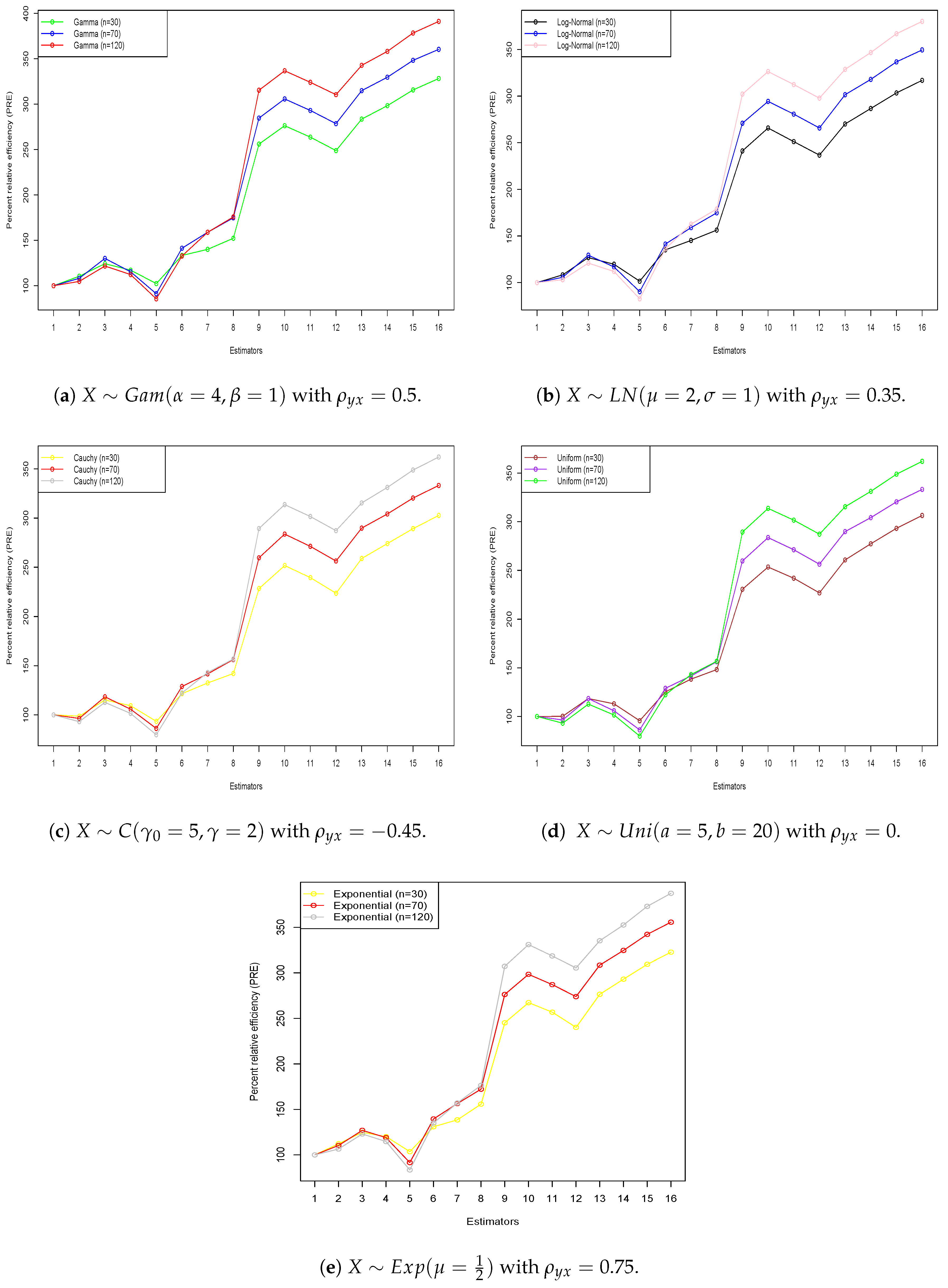
6.1. Simulation Study

The nature of the data and the statistical characteristics of the distribution determine which distribution is most suited for a median estimate; the median is especially useful and compatible with skewed distributions, contains outliers, and has non-normal characteristics. Positively skewed distributions were used to evaluate the performance of the proposed estimators under conditions where the data deviate from normality, which is common in many practical survey scenarios. We selected the given five distributions to obtain the variable X:

• Population 1: $X\sim$ Moderate skew and spread Gamma distribution $(\alpha =4,\beta =1)$ with ${\rho }_{yx}=0.5;$
• Population 2: $X\sim$ Slight skew Log-Normal distribution $(\mu =2,\sigma =1)$ with ${\rho }_{yx}=0.35;$
• Population 3: $X\sim$ Heavy tails Cauchy distribution $({\gamma }_0=5,\gamma =2)$ with ${\rho }_{yx}=-0.45;$
• Population 4: $X\sim$ Baseline Uniform distribution $(a=5,b=20)$ with ${\rho }_{yx}=0;$
• Population 5: $X\sim$ High skew Exponential $(\mu ={\displaystyle \frac{1}{2}})$ with ${\rho }_{yx}=0.75.$

These five distributions are most suited for testing and proving the robustness of the suggested estimators under conditions and their characteristics: We can determine the variable Y through the expression given below:

$$Y=r_{yx}\times X+e,$$

where $r_{yx}$ is the correlation, and

$$e\sim N(0,1),$$

represents the error term.

In order to evaluate robustness and efficiency, we applied the following methods to the R program and examined the MSEs of the various suggested estimators and other existing estimators for every distribution and correlation setting.

(1) Generate populations: Using the techniques described above, simulate $N=900$ observations for X and $Y.$

(2) Sample selection: Samples of size n can be chosen using simple random sampling without replacement (SRSWOR). The sample sizes are $n=30,70,$ and 120.

(3) Optimal parameter estimation: To assess and check the performance of the estimators, compute the required statistics (such as sample mean, median, variance, and covariance) from the sampled data using the procedures outlined above. The optimal values for the enhanced class of estimators, which consider unknown constants along, are also determined.

(4) Performance Metrics: For every sample size, the efficiency ($PRE$) values for each estimator discussed in this article are computed.

(5) Replications: After 85,000 iterations of steps 3 and 4, compute the mean squared errors and percent relative efficiency using the formulas provided below:

$$MSE{\left({\widehat{M}}_t\right)}_{min}={\displaystyle \frac{{\sum }_{k=1}^{85000}{\left({\widehat{M}}_{tk}-M_y\right)}^2}{85000}}$$

and

$$PRE={\displaystyle \frac{Var\left({\widehat{M}}_y\right)}{MSE{\left({\widehat{M}}_t\right)}_{min}}}\times 100,$$

where $t=R,D,Re,Pe,D_1,D_2{D}_3,U_1,U_2,\dots ,U_8.$

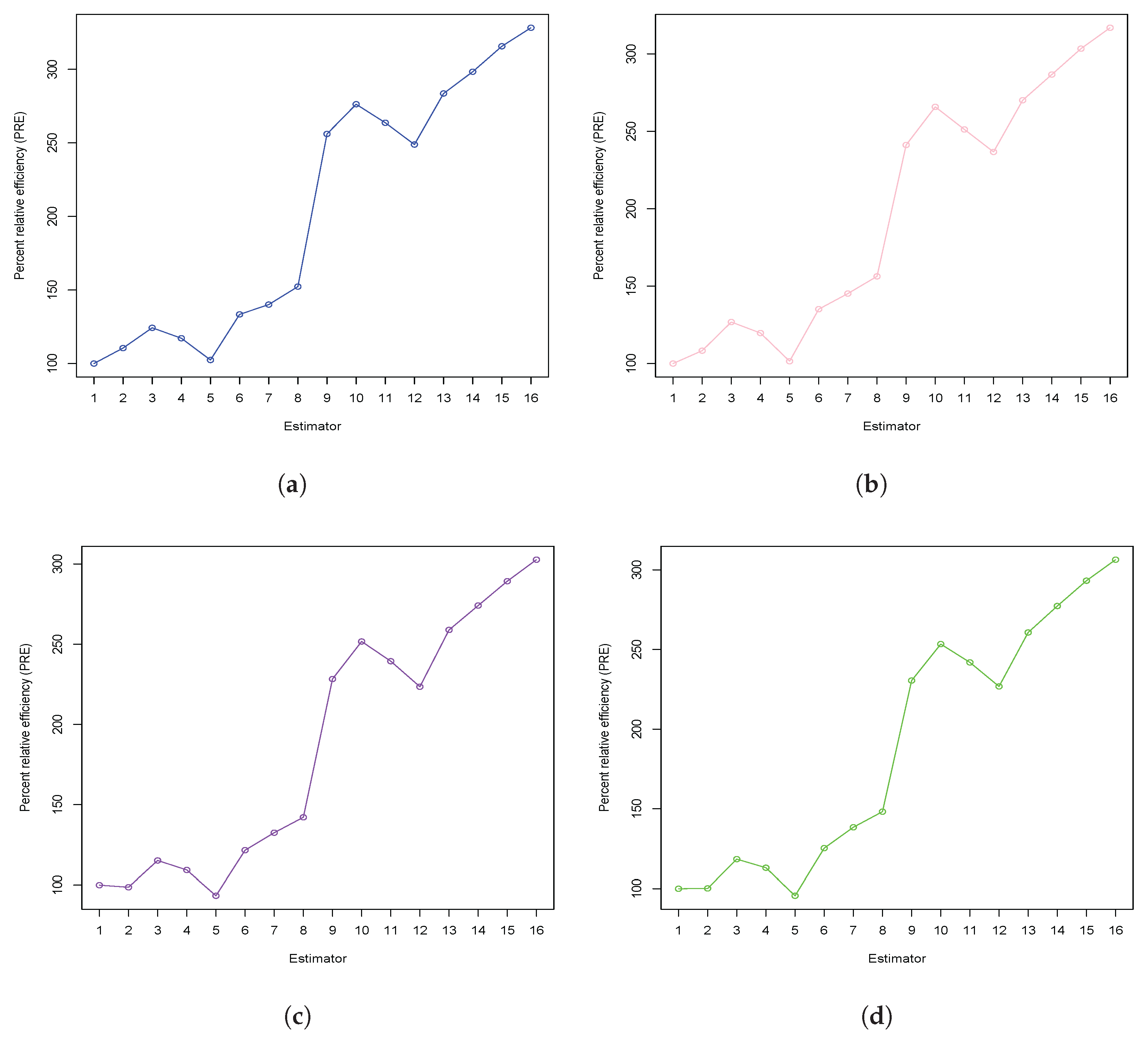
6.2. Real-Life Application

We now examine the percent relative efficiency (PRE) of three distinct data sets, helping us to evaluate the performance of the proposed family of estimators as compared to other different estimators. The data sets and their main statistical summaries are described in detail below,

Population 1 

(Source: Singh [10]).

Y: represents the total quantity of fish that was caught in 1995;

$X:$ represents the total quantity of fish caught by marine recreational fishermen in 1994.

$$\begin{array}{c}N=69,n=17,M_x=2011,M_y=2068,f_x\left(M_x\right)=0.00014,f_y\left(M_y\right)=0.00014,{\rho }_{yx}=0.151,\hfill \\ T_M=4043,D_M=3853,Q_R=3936,Q_A=2956,Q_D=1968,M_R=19019.5.\hfill \end{array}$$

Population 2 

(Source: Murthy [29]).

$Y:$ denotes the total number of households;

$X:$ denotes the total area in square miles.

$$\begin{array}{c}N=128,n=45,M_x=4.715,M_y=686,f_x\left(M_x\right)=0.1154,f_y\left(M_y\right)=0.00092,{\rho }_{yx}=0.468,\hfill \\ T_M=5.385,D_M=5.378,Q_R=4.618,Q_A=5.316,Q_D=2.309,M_R=8.270.\hfill \end{array}$$

Population 3 

(Source: Koyuncu and Kadilar [30]).

$Y:$ denotes the total number of teachers in educational institutions;

$X:$ denotes the total number of students enrolled in educational institutions in 2012.

$$\begin{array}{c}N=923,n=180,M_x=4123,M_y=171,f_x\left(M_x\right)=0.00009409,f_y\left(M_y\right)=0.002676,\hfill \\ {\rho }_{yx}=0.855,T_M=7726,D_M=7348.3,Q_R=8283,Q_A=5870.5,Q_D=4141.5,M_R=89530.\hfill \end{array}$$

Population 4 

(Source: Singh [10]).

Y: represents the total quantity of fish that was caught in 1995;

$X:$ represents the total quantity of fish caught by marine recreational fishermen in 1934.

$$\begin{array}{c}N=69,n=17,M_x=2007,M_y=2068,f_x\left(M_x\right)=0.00014,f_y\left(M_y\right)=0.00014,{\rho }_{yx}=0.314,\hfill \\ T_M=3777,D_M=3615.2,Q_R=3936,Q_A=3002,Q_D=1975,M_R=17030.\hfill \end{array}$$

Now, we calculate the efficiency for each estimator by using the formulas expressed below:

$$PRE={\displaystyle \frac{Var\left({\widehat{M}}_y\right)}{MSE\left({\widehat{M}}_v\right)}}\times 100,$$

where $v=R,D,Re,Pe,D_1,D_2{D}_3,U_1,U_2,\dots ,U_8.$ The results of this analysis, which highlight the performance of our proposed family of estimators, can be found in Table 5.

6.3. Discussion

To support the median estimations, we conducted simulations using suitable distributions with varying ${\rho }_{yx}$ values and different sample sizes. We also examined four data sets to assess the performance of the suggested family of estimators. Our main criterion for comparing the various estimators was the percent relative efficiency criterion (PRE). Table 2, Table 3 and Table 4 present the PRE values for the new family and other existing estimators from five simulated distributions. In Table 5, the results from the actual data sets are displayed. We derive the following significant conclusions from these analyses:

• The $PRE$ values for all new estimators are higher than those of the other existing estimators covered in Section 2, according to the findings of both simulated and real data sets, which are shown in Table 2, Table 3, Table 4 and Table 5. This illustrates the better performance of the newly proposed estimators over existing ones.
• Furthermore, the upward-trending graph lines in Figure 1 and Figure 2 for both five simulated distributions and four real data sets prove that all new estimators have $PRE$ values that are consistently greater than those of existing estimators. The inverse relationship between the $PRE$ values for the new estimators and the existing estimators led to the conclusion that the new family of estimators outperforms existing methods. This proves that the proposed family of estimators performs better than the other estimators, as it shows a reverse relationship between the $MSE$ values for the new and existing approaches.
• Based on the comprehensive simulation results and real-life data analysis presented in Table 2, Table 3, Table 4 and Table 5, the estimator ${\widehat{M}}_{U_8}$ consistently demonstrates the highest percent relative efficiency (PRE) among all proposed and existing estimators. Therefore, we recommend the use of ${\widehat{M}}_{U_8}$ in practice, especially in applications involving skewed or data affected by extreme under simple random sampling.

Table 2. Percent relative efficiency (PRE) for $n=30$.

Estimator	$\mathit{Gam}(4,1)$	$\mathit{LN}(2,1)$	$\mathit{C}(5,2)$	$\mathit{Uni}(5,20)$	$\mathit{Exp}\left(0.5\right)$
${\widehat{M}}_y$	100.00	100.00	100.00	100.00	100.00
${\widehat{M}}_R$	110.54	108.31	98.70	100.29	112.39
${\widehat{M}}_D$	124.37	126.80	115.21	118.43	124.80
${\widehat{M}}_{Re}$	117.21	119.79	109.35	113.01	120.12
${\widehat{M}}_{Pe}$	102.46	101.57	93.46	95.68	103.61
${\widehat{M}}_{D_1}$	133.41	135.12	121.60	125.30	131.35
${\widehat{M}}_{D_2}$	140.10	145.97	132.50	138.47	138.55
${\widehat{M}}_{D_3}$	152.32	156.37	142.17	148.28	155.80
${\widehat{M}}_{U_1}$	256.17	241.29	228.36	230.54	245.23
${\widehat{M}}_{U_2}$	276.30	265.81	251.71	253.48	267.34
${\widehat{M}}_{U_3}$	263.73	251.27	239.49	241.96	256.88
${\widehat{M}}_{U_4}$	248.97	236.70	223.54	226.83	240.15
${\widehat{M}}_{U_5}$	283.61	270.10	258.46	260.77	276.52
${\widehat{M}}_{U_6}$	298.46	286.75	274.17	277.35	293.19
${\widehat{M}}_{U_7}$	315.70	303.46	289.33	293.29	309.45
${\widehat{M}}_{U_8}$	328.33	316.95	302.73	306.48	322.86

Table 2. Percent relative efficiency (PRE) for $n=30$.

Estimator	$\mathit{Gam}(4,1)$	$\mathit{LN}(2,1)$	$\mathit{C}(5,2)$	$\mathit{Uni}(5,20)$	$\mathit{Exp}\left(0.5\right)$
${\widehat{M}}_y$	100.00	100.00	100.00	100.00	100.00
${\widehat{M}}_R$	110.54	108.31	98.70	100.29	112.39
${\widehat{M}}_D$	124.37	126.80	115.21	118.43	124.80
${\widehat{M}}_{Re}$	117.21	119.79	109.35	113.01	120.12
${\widehat{M}}_{Pe}$	102.46	101.57	93.46	95.68	103.61
${\widehat{M}}_{D_1}$	133.41	135.12	121.60	125.30	131.35
${\widehat{M}}_{D_2}$	140.10	145.97	132.50	138.47	138.55
${\widehat{M}}_{D_3}$	152.32	156.37	142.17	148.28	155.80
${\widehat{M}}_{U_1}$	256.17	241.29	228.36	230.54	245.23
${\widehat{M}}_{U_2}$	276.30	265.81	251.71	253.48	267.34
${\widehat{M}}_{U_3}$	263.73	251.27	239.49	241.96	256.88
${\widehat{M}}_{U_4}$	248.97	236.70	223.54	226.83	240.15
${\widehat{M}}_{U_5}$	283.61	270.10	258.46	260.77	276.52
${\widehat{M}}_{U_6}$	298.46	286.75	274.17	277.35	293.19
${\widehat{M}}_{U_7}$	315.70	303.46	289.33	293.29	309.45
${\widehat{M}}_{U_8}$	328.33	316.95	302.73	306.48	322.86

Table 3. Percent relative efficiency (PRE) for $n=70$.

Estimator	$\mathit{Gam}(4,1)$	$\mathit{LN}(2,1)$	$\mathit{C}(5,2)$	$\mathit{Uni}(5,20)$	$\mathit{Exp}\left(0.5\right)$
${\widehat{M}}_y$	100.00	100.00	100.00	100.00	100.00
${\widehat{M}}_R$	108.21	105.78	96.41	97.57	110.46
${\widehat{M}}_D$	130.15	129.42	118.41	120.82	127.41
${\widehat{M}}_{Re}$	115.49	116.88	105.82	109.23	119.08
${\widehat{M}}_{Pe}$	91.24	90.37	86.27	88.38	91.60
${\widehat{M}}_{D_1}$	141.30	141.31	128.94	132.56	139.50
${\widehat{M}}_{D_2}$	158.98	158.94	141.75	147.39	156.48
${\widehat{M}}_{D_3}$	174.83	174.87	156.34	161.26	172.28
${\widehat{M}}_{U_1}$	284.72	270.95	259.60	261.86	276.36
${\widehat{M}}_{U_2}$	305.84	294.39	283.74	285.64	298.42
${\widehat{M}}_{U_3}$	293.14	280.76	271.28	272.92	287.15
${\widehat{M}}_{U_4}$	278.69	265.84	256.36	259.22	273.96
${\widehat{M}}_{U_5}$	314.94	301.55	289.83	292.31	308.52
${\widehat{M}}_{U_6}$	329.79	317.90	304.27	307.13	324.72
${\widehat{M}}_{U_7}$	348.39	336.77	320.41	323.45	342.33
${\widehat{M}}_{U_8}$	360.40	349.58	333.25	337.64	355.72

Table 3. Percent relative efficiency (PRE) for $n=70$.

Estimator	$\mathit{Gam}(4,1)$	$\mathit{LN}(2,1)$	$\mathit{C}(5,2)$	$\mathit{Uni}(5,20)$	$\mathit{Exp}\left(0.5\right)$
${\widehat{M}}_y$	100.00	100.00	100.00	100.00	100.00
${\widehat{M}}_R$	108.21	105.78	96.41	97.57	110.46
${\widehat{M}}_D$	130.15	129.42	118.41	120.82	127.41
${\widehat{M}}_{Re}$	115.49	116.88	105.82	109.23	119.08
${\widehat{M}}_{Pe}$	91.24	90.37	86.27	88.38	91.60
${\widehat{M}}_{D_1}$	141.30	141.31	128.94	132.56	139.50
${\widehat{M}}_{D_2}$	158.98	158.94	141.75	147.39	156.48
${\widehat{M}}_{D_3}$	174.83	174.87	156.34	161.26	172.28
${\widehat{M}}_{U_1}$	284.72	270.95	259.60	261.86	276.36
${\widehat{M}}_{U_2}$	305.84	294.39	283.74	285.64	298.42
${\widehat{M}}_{U_3}$	293.14	280.76	271.28	272.92	287.15
${\widehat{M}}_{U_4}$	278.69	265.84	256.36	259.22	273.96
${\widehat{M}}_{U_5}$	314.94	301.55	289.83	292.31	308.52
${\widehat{M}}_{U_6}$	329.79	317.90	304.27	307.13	324.72
${\widehat{M}}_{U_7}$	348.39	336.77	320.41	323.45	342.33
${\widehat{M}}_{U_8}$	360.40	349.58	333.25	337.64	355.72

Table 4. Percent relative efficiency (PRE) for $n=120$.

Estimator	$\mathit{Gam}(4,1)$	$\mathit{LN}(2,1)$	$\mathit{C}(5,2)$	$\mathit{Uni}(5,20)$	$\mathit{Exp}\left(0.5\right)$
${\widehat{M}}_y$	100.00	100.00	100.00	100.00	100.00
${\widehat{M}}_R$	104.81	103.17	93.120	95.56	106.50
${\widehat{M}}_D$	121.71	120.93	112.72	115.24	123.77
${\widehat{M}}_{Re}$	112.33	111.97	101.59	105.70	114.77
${\widehat{M}}_{Pe}$	85.66	82.68	79.81	81.28	83.51
${\widehat{M}}_{D_1}$	132.79	136.11	122.30	127.84	135.13
${\widehat{M}}_{D_2}$	158.91	162.72	143.18	150.27	157.07
${\widehat{M}}_{D_3}$	175.80	178.90	156.85	164.76	176.41
${\widehat{M}}_{U_1}$	315.48	302.18	289.43	291.64	307.25
${\widehat{M}}_{U_2}$	336.86	326.38	313.78	316.23	331.14
${\widehat{M}}_{U_3}$	324.14	312.44	301.65	303.52	318.65
${\widehat{M}}_{U_4}$	310.53	297.81	287.23	290.16	305.44
${\widehat{M}}_{U_5}$	342.82	328.78	315.48	319.80	335.31
${\widehat{M}}_{U_6}$	358.27	346.74	331.29	335.44	352.61
${\widehat{M}}_{U_7}$	378.44	366.92	348.93	352.75	373.17
${\widehat{M}}_{U_8}$	391.20	380.18	362.10	366.54	387.48

Table 4. Percent relative efficiency (PRE) for $n=120$.

Estimator	$\mathit{Gam}(4,1)$	$\mathit{LN}(2,1)$	$\mathit{C}(5,2)$	$\mathit{Uni}(5,20)$	$\mathit{Exp}\left(0.5\right)$
${\widehat{M}}_y$	100.00	100.00	100.00	100.00	100.00
${\widehat{M}}_R$	104.81	103.17	93.120	95.56	106.50
${\widehat{M}}_D$	121.71	120.93	112.72	115.24	123.77
${\widehat{M}}_{Re}$	112.33	111.97	101.59	105.70	114.77
${\widehat{M}}_{Pe}$	85.66	82.68	79.81	81.28	83.51
${\widehat{M}}_{D_1}$	132.79	136.11	122.30	127.84	135.13
${\widehat{M}}_{D_2}$	158.91	162.72	143.18	150.27	157.07
${\widehat{M}}_{D_3}$	175.80	178.90	156.85	164.76	176.41
${\widehat{M}}_{U_1}$	315.48	302.18	289.43	291.64	307.25
${\widehat{M}}_{U_2}$	336.86	326.38	313.78	316.23	331.14
${\widehat{M}}_{U_3}$	324.14	312.44	301.65	303.52	318.65
${\widehat{M}}_{U_4}$	310.53	297.81	287.23	290.16	305.44
${\widehat{M}}_{U_5}$	342.82	328.78	315.48	319.80	335.31
${\widehat{M}}_{U_6}$	358.27	346.74	331.29	335.44	352.61
${\widehat{M}}_{U_7}$	378.44	366.92	348.93	352.75	373.17
${\widehat{M}}_{U_8}$	391.20	380.18	362.10	366.54	387.48

Table 5. Percent relative efficiency (PRE) of different estimators using real populations.

Estimator	Data 1	Data 2	Data 3	Data 4
${\widehat{M}}_y$	100.00	100.00	100.00	100.00
${\widehat{M}}_R$	110.50	108.33	98.74	100.28
${\widehat{M}}_D$	124.33	126.80	115.23	118.46
${\widehat{M}}_{Re}$	117.29	119.71	109.35	113.03
${\widehat{M}}_{Pe}$	102.48	101.52	93.46	95.64
${\widehat{M}}_{D_1}$	133.47	135.13	121.67	125.35
${\widehat{M}}_{D_2}$	140.16	145.24	132.58	138.46
${\widehat{M}}_{D_3}$	152.35	156.35	142.19	148.27
${\widehat{M}}_{U_1}$	256.14	241.26	228.30	230.58
${\widehat{M}}_{U_2}$	276.33	265.87	251.75	253.49
${\widehat{M}}_{U_3}$	263.72	251.28	239.44	241.90
${\widehat{M}}_{U_4}$	248.91	236.79	223.53	226.85
${\widehat{M}}_{U_5}$	283.60	270.12	258.92	260.74
${\widehat{M}}_{U_6}$	298.44	286.75	274.11	277.34
${\widehat{M}}_{U_7}$	315.77	303.48	289.36	293.23
${\widehat{M}}_{U_8}$	328.37	316.93	302.78	306.42

Table 5. Percent relative efficiency (PRE) of different estimators using real populations.

Estimator	Data 1	Data 2	Data 3	Data 4
${\widehat{M}}_y$	100.00	100.00	100.00	100.00
${\widehat{M}}_R$	110.50	108.33	98.74	100.28
${\widehat{M}}_D$	124.33	126.80	115.23	118.46
${\widehat{M}}_{Re}$	117.29	119.71	109.35	113.03
${\widehat{M}}_{Pe}$	102.48	101.52	93.46	95.64
${\widehat{M}}_{D_1}$	133.47	135.13	121.67	125.35
${\widehat{M}}_{D_2}$	140.16	145.24	132.58	138.46
${\widehat{M}}_{D_3}$	152.35	156.35	142.19	148.27
${\widehat{M}}_{U_1}$	256.14	241.26	228.30	230.58
${\widehat{M}}_{U_2}$	276.33	265.87	251.75	253.49
${\widehat{M}}_{U_3}$	263.72	251.28	239.44	241.90
${\widehat{M}}_{U_4}$	248.91	236.79	223.53	226.85
${\widehat{M}}_{U_5}$	283.60	270.12	258.92	260.74
${\widehat{M}}_{U_6}$	298.44	286.75	274.11	277.34
${\widehat{M}}_{U_7}$	315.77	303.48	289.36	293.23
${\widehat{M}}_{U_8}$	328.37	316.93	302.78	306.42

6.3.1. Limitations of the Proposed Estimator

Although the proposed family of estimators demonstrates improved efficiency in terms of bias and percent relative efficiency (PRE), particularly for skewed distributions, it has some practical limitations:

• Dependence on auxiliary information: The performance improvements depend strongly on the availability and quality of auxiliary variables. If the auxiliary variable exhibits a weak correlation with the study variable, or if its distributional characteristics are poorly understood, the proposed estimators may not yield significant benefits.
• Computational complexity: Unlike traditional estimators such as the sample median or ratio-type estimators, the proposed estimators require more elaborate computations. These include transformation functions and the estimation of tuning parameters (such as $k_1$ and $k_2$), which may be less practical in time-constrained or resource-limited survey environments.
• Assumption of known robust parameters: The proposed estimators use robust statistics like the interquartile range, trimean, or decile mean, assuming that such measures are either available from prior knowledge or can be estimated accurately. In scenarios where this information is unavailable or unreliable, the estimator’s effectiveness could be limited.

6.3.2. Applicability of the Proposed Estimators in Practical Scenarios

The proposed family of estimators is particularly useful in the following applied settings:

• Skewed distributions: In surveys involving variables such as income, expenditures, or environmental indicators that typically show non-normal or skewed distributions, the proposed estimators outperform traditional alternatives by offering greater robustness.
• Presence of outliers: In data sets that contain outliers or extreme values, traditional estimators may be heavily influenced, whereas the proposed estimators, which are designed using robust transformations, continue to provide reliable median estimates.
• Moderate to strong auxiliary variable correlation: When the auxiliary variable is moderately or strongly correlated with the study variable, the proposed estimators achieve high percent relative efficiency (PRE), as supported by both simulation results and real-data applications in the manuscript.

7. Conclusions and Future Works

In this work, we used robust measurements of an auxiliary variable to obtain a new family of estimators for estimating the finite population median under simple random sampling. The first degree of approximation was used to obtain the biases, mean squared errors (MSEs), and minimum MSE of the new family of estimators. To compare the potential performance of new estimators with existing estimators using the percent relative efficiency criterion, we performed a simulation analysis using five distributions with all effective conditions and four real data sets. The simulation and numerical real-life data set results are given in Table 2, Table 3, Table 4 and Table 5, which show that the new family of estimators performs well and can obtain the optimum estimators as compared to other existing estimators. While all of the new estimators have a higher percent relative efficiency than other estimators, the proposed estimator ${\widehat{M}}_{U_8}$ is the best option among the proposed family of estimators and is thus strongly recommended.

Furthermore, our analysis focused on the properties of the new family of estimators within the context of simple random sampling. It is worth exploring the potential of developing new estimators based on these findings; we can extend these results to some other sampling techniques, such as finite population median using stratified random sampling, rank set sampling, finite population proportions, and population medians in the presence of non-sampling errors.

References

1. Cochran, W.B. Sampling Techniques; John Wiley and Sons: Hoboken, NJ, USA, 1963. [Google Scholar]
2. Särndal, C.E. Sample survey theory vs. general statistical theory: Estimation of the population mean. Int. Stat. Rev. Int. Stat. 1972, 40, 1–12. [Google Scholar] [CrossRef]
3. Gross, S. Median estimation in sample surveys. In Proceedings of the Section on Survey Research Methods; American Statistical Association Ithaca: Alexandria, VA, USA, 1980. [Google Scholar]
4. Sedransk, J.; Meyer, J. Confidence intervals for the quantiles of a finite population: Simple random and stratified simple random sampling. J. R. Stat. Soc. Ser. B 1978, 40, 239–252. [Google Scholar] [CrossRef]
5. Philip, S.; Sedransk, J. Lower bounds for confidence coefficients for confidence intervals for finite population quantiles. Commun. Stat. Theory Methods 1983, 12, 1329–1344. [Google Scholar] [CrossRef]
6. Kuk, Y.C.A.; Mak, T.K. Median estimation in the presence of auxiliary information. J. R. Stat. Soc. Ser. B 1989, 51, 261–269. [Google Scholar] [CrossRef]
7. Rao, T.J. On certail methods of improving ration and regression estimators. Commun. Stat. Theory Methods 1991, 20, 3325–3340. [Google Scholar] [CrossRef]
8. Singh, S.; Joarder, A.H.; Tracy, D.S. Median estimation using double sampling. Aust. N. Z. J. Stat. 2001, 43, 33–46. [Google Scholar] [CrossRef]
9. Khoshnevisan, M.; Singh, H.P.; Singh, S.; Smarandache, F. A General Class of Estimators of Population Median Using Two Auxiliary Variables in Double Sampling; Virginia Polytechnic Institute and State University: Blacksburg, VA, USA, 2002. [Google Scholar]
10. Singh, S. Advanced Sampling Theory with Applications: How Michael Selected Amy; Springer Science & Business Media: Berlin/Heidelberg, Germany, 2003; Volume 2. [Google Scholar]
11. Gupta, S.; Shabbir, J.; Ahmad, S. Estimation of median in two-phase sampling using two auxiliary variables. Commun. Stat. Theory Methods 2008, 37, 1815–1822. [Google Scholar] [CrossRef]
12. Aladag, S.; Cingi, H. Improvement in estimating the population median in simple random sampling and stratified random sampling using auxiliary information. Commun. Stat. Theory Methods 2015, 44, 1013–1032. [Google Scholar] [CrossRef]
13. Solanki, R.S.; Singh, H.P. Some classes of estimators for median estimation in survey sampling. Commun. Stat. Theory Methods 2015, 44, 1450–1465. [Google Scholar] [CrossRef]
14. Daraz, U.; Khan, M. Estimation of variance of the difference-cum-ratio-type exponential estimator in simple random sampling. Res. Math. Stat. 2021, 8, 1899402. [Google Scholar] [CrossRef]
15. Daraz, U.; Alomair, M.A.; Albalawi, O. Variance estimation under some transformation for both symmetric and asymmetric data. Symmetry 2024, 16, 957. [Google Scholar] [CrossRef]
16. Ding, F. Least squares parameter estimation and multi-innovation least squares methods for linear fitting problems from noisy data. J. Comput. Appl. Math. 2023, 426, 115107. [Google Scholar] [CrossRef]
17. Shabbir, J.; Gupta, S. A generalized class of difference type estimators for population median in survey sampling. Hacet. J. Math. Stat. 2017, 46, 1015–1028. [Google Scholar] [CrossRef]
18. Irfan, M.; Maria, J.; Shongwe, S.C.; Zohaib, M.; Bhatti S., H. Estimation of population median under robust measures of an auxiliary variable. Math. Probl. Eng. 2021, 2021, 4839077. [Google Scholar] [CrossRef]
19. Shabbir, J.; Gupta, S.; Narjis, G. On improved class of difference type estimators for population median in survey sampling. Commun. Stat. Theory Methods 2022, 51, 3334–3354. [Google Scholar] [CrossRef]
20. Subzar, M.; Lone, S.A.; Ekpenyong, E.J.; Salam, A.; Aslam, M.; Raja, T.A.; Almutlak, S.A. Efficient class of ratio cum median estimators for estimating the population median. PLoS ONE 2023, 18, e0274690. [Google Scholar] [CrossRef] [PubMed]
21. Iseh, M.J. Model formulation on efficiency for median estimation under a fixed cost in survey sampling. Model Assist. Stat. Appl. 2023, 18, 373–385. [Google Scholar] [CrossRef]
22. Hussain, M.A.; Javed, M.; Zohaib, M.; Shongwe, S.C.; Awais, M.; Zaagan, A.A.; Irfan, M. Estimation of population median using bivariate auxiliary information in simple random sampling. Heliyon 2024, 10, e28891. [Google Scholar] [CrossRef]
23. Almulhim, F.A.; Alghamdi, A.S. Simulation-based evaluation of robust transformation techniques for median estimation under simple random sampling. Axioms 2025, 14, 301. [Google Scholar] [CrossRef]
24. Baig, A.; Masood, S.; Ahmed Tarray, T. Improved class of difference-type estimators for population median in survey sampling. Commun. Stat. Theory Methods 2019, 49, 5778–5793. [Google Scholar] [CrossRef]
25. Masood, S.; Ibrar, B.; Shabbir, J.; Movaheedil, Z. Estimating neutrosophic finite median employing robust measures of the auxiliary variable. Sci. Rep. 2024, 14, 10255. [Google Scholar] [CrossRef] [PubMed]
26. Daraz, U.; Alomair, M.A.; Albalawi, O.; Al Naim, A.S. New Techniques for Estimating Finite Population Variance Using Ranks of Auxiliary Variable in Two-Stage Sampling. Mathematics 2024, 12, 2741. [Google Scholar] [CrossRef]
27. Alomair, M.A.; Daraz, U. Dual transformation of auxiliary variables by using outliers in stratified random sampling. Mathematics 2024, 12, 2829. [Google Scholar] [CrossRef]
28. Singh, H.P.; Vishwakarma, G.K. Modified exponential ratio and product estimators for finite population mean in double sampling. Austrian J. Stat. 2007, 36, 217–225. [Google Scholar] [CrossRef]
29. Murthy, M.N. Sampling Theory and Methods; Statistical Publishing Society: Calcutta, India, 1967. [Google Scholar]
30. Koyuncu, K.; Kadilar, C. Family of estimators of population mean using two auxiliary variables in stratified random sampling. Commun. Stat. Theory Methods 2009, 38, 2398–2417. [Google Scholar] [CrossRef]
Figure 1. A graphical display of the findings utilizing information obtained from different population distributions.
Mathematics 13 01660 g001
Figure 2. A graphical display of the findings utilizing information obtained from different data sets. (a) Source: [10]. (b) Source: [29]. (c) Source: [30]. (d) Source: [10].
Mathematics 13 01660 g002