Abstract
This study proposes a mixed-integer programming-based hierarchical collaborative optimization (MIP-HCO) model to optimize the scheduling and execution of emergency launch missions, ensuring rapid response and performance maximization under constrained time and resources. The key innovation lies in integrating k-Nearest Neighbor (KNN) with Branch and Bound (B&B) to enhance computational efficiency and global optimality. The first layer constructs a spatiotemporal optimization model, considering launch sites, storage proximity, and process duration. The B&B algorithm solves mission scheduling, while a dynamic adjustment strategy optimizes launch vehicle reutilization. The second layer refines mission selection based on contribution assessment and re-optimizes scheduling using integer programming. KNN classification approximates scheduling quality, reducing B&B complexity and accelerating convergence. Results from simulation data and experimental simulations confirm that the KNN + B&B hybrid strategy optimizes scheduling efficiency, enabling launch systems to respond swiftly under emergencies while maximizing mission effectiveness.
Keywords:
mixed-integer programming; branch and bound; k-nearest neighbors; aerospace emergency launch MSC:
90C57; 65K10; 68T20
1. Introduction
The aerospace industry, as a significant embodiment of a nation’s comprehensive national strength, plays a pivotal role in the process of modern technological development. Aerospace emergency launch is a special launch activity that uses dedicated rockets to launch satellites, such as reserve satellites, into space from emergency launch sites outside of regular launch bases [1]. This type of launch plays a critical role in emergency situations, including missions like network replenishment, network reconfiguration, and regional enhancement, and has become a key component of aerospace launch and recovery forces. Through emergency launches, rapid responses to joint operations and space warfare needs can be achieved, ensuring strategic advantages in entering, utilizing, and controlling space. This method holds significant military value and is an important manifestation of new operational capabilities [2]. The main challenges in emergency launch mission planning include the limited launch windows, the urgency of time scheduling, and the complexity of resource scheduling [3,4,5]. For aerospace emergency launch missions, it is typically necessary to construct an integrated operational process that includes “transportation-testing-launch-evaluation”. Under the constraints of limited launch windows, time windows, and construction resources, how to achieve multiple launch objectives within the specified time, while maximizing mission contribution and ensuring mission execution efficiency, is a critical issue that needs to be addressed.
In recent years, mission planning research in the aerospace field has gradually become a focal point, with the primary focus on key aspects such as mission planning, launch procedures, and resource management. In terms of mission planning, the research covers launch objective planning, trajectory planning, path planning, action planning, and launch time analysis. In response to unexpected mission interruption scenarios [6,7], a redundancy-based mission chain generation approach using reinforcement learning can be employed to ensure rapid reconfiguration of in-orbit resources and maintain mission continuity. Aiming to achieve rapid and precise mission planning based on different mission scenarios. Research on launch procedures focuses on optimizing the launch process to improve launch efficiency and response speed, including the design of emergency launch procedures based on storage status. In addition, a risk-driven multi-objective optimization model can be introduced to quantify environmental disturbances and equipment failure risks as dynamic constraints. By integrating the Fuzzy Analytic Hierarchy Process (FAHP) [8,9] with Bayesian Networks [10], the model enables real-time updates of risk weights, thereby generating resilient mission paths that balance efficiency and robustness [11].
The contributions of this study are summarized as follows:
- 1.
- Innovation in Bi-level Collaborative Optimization Framework:This study proposes a dual-layer mixed-integer programming hybrid collaborative optimization (MIP-HCO) model that decouples spatiotemporal and mission-related considerations. In the spatiotemporal coordination layer, the introduction of conflict time window constraints and path deviation limitations generates a conflict-free baseline solution, ensuring the feasibility and coordination of missions in both time and space. In the mission optimization layer, the model dynamically selects high-contribution mission combinations, enhancing the overall value of the missions. This effectively addresses the multi-objective coupling challenge, achieving an optimized balance between mission priority evaluation and resource allocation.
- 2.
- Enhancement of Dynamic Scheduling Efficiency: Under stringent time constraints, the proposed method significantly improves mission completion efficiency while effectively reducing redundancy and conflicts in resource scheduling. By optimizing the scheduling scheme, the model achieves substantial improvements in mission timeliness, resource utilization, and execution efficiency. It provides an efficient and coordinated “time-resource-efficiency” balance solution, making it particularly suitable for emergency mission scheduling.
- 3.
- KNN + B&B Computational Optimization Enhancement: This study integrates the k-Nearest Neighbor (KNN) classification algorithm with the Branch and Bound (B&B) method, effectively reducing computational complexity and improving convergence speed. By introducing a machine learning-assisted branch selection mechanism, KNN predicts the quality of candidate scheduling solutions during the B&B search process, prioritizing the expansion of branches with higher potential. This accelerates the scheduling optimization process and significantly enhances the model’s real-time adaptability in complex emergency scenarios, providing a more efficient and intelligent solution framework.
The structure of this paper is as follows: Section 2 presents related work. Section 3 provides an overview of the problem statement and the definition of notations. Section 4 elaborates on the MIP-HCO model. Section 5 presents the computational results and visual representations of the model. Section 6 validates the advantages of the proposed model over traditional algorithms through comparative experiments. Section 7 discusses the model analysis and extensions. Section 8 discusses the significance of the model in the research context. Section 9 concludes the paper with a summary of findings.
2. Related Work
The research on aerospace emergency launch missions encompasses multiple aspects, including launch window analysis, resource scheduling optimization, mission planning, and scheme evaluation. Scholars both domestically and internationally have conducted extensive studies in this field.
2.1. Theoretical Analysis of Launch Windows
In aerospace emergency missions, the calculation of the launch window is crucial as it directly impacts the feasibility and efficiency of the mission. Early studies primarily focused on the time constraints in rendezvous and docking missions. In his seminal work [12], Marshall H. Kaplan explored the key constraints affecting satellites during rendezvous and docking operations, linking these constraints to launch timing. His in-depth analysis of launch window computation methods laid a theoretical foundation for subsequent research. Houin et al. [13] investigated the constraints of rendezvous and docking for Artemis III and subsequent missions in Near-Rectilinear Halo Orbit (NRHO). They constructed a mathematical model for launch timing and utilized contour plots to analyze costs under varying launch dates and transfer durations. Their approach successfully generated continuous launch windows, ensuring an optimal transfer configuration on a daily basis. Brandimarte [14], in their study on emergency launch mission planning for high-orbit satellites, adopted an optimization approach similar to the Mixed-Integer Linear Programming (MILP) model to adjust orbital change strategies. They proposed a launch window optimization model that accounts for resource constraints, mission priority, and cost-effectiveness under dynamic mission demands. By utilizing MILP-based multi-constraint scheduling, their approach optimizes launch mission feasibility and enhances overall mission benefits. These studies provide a theoretical foundation for launch window design in deep space exploration missions.
2.2. Resource Scheduling and Optimization
With the increasing complexity of space missions, resource scheduling has become a focal point of research. Zhang et al. [15] proposed a satellite control resource scheduling method based on the Ant Colony Optimization (ACO) algorithm. This method optimizes the allocation of satellite resources by simplifying the pheromone model and fixing the pheromone range, thereby enhancing the workload efficiency of the TT&C (Telemetry, Tracking, and Command) network. The research provides decision-making support for resource scheduling and optimization in aerospace missions. Wang et al. [16] proposed an Integer Linear Programming (ILP) optimization model based on the Event-Driven Time Expansion Graph (EDTEG) to maximize the total priority of successfully scheduled missions. Their approach improves mission success rates and reduces resource conflicts in multi-resource coordinated scheduling problems. Furthermore, Chen et al. [17] proposed an Efficient Resource Scheduling (TRS) algorithm based on TVRG, which features a multi-level on-demand scheduling capability, enhancing resource utilization efficiency.
2.3. Emergency Launch Mission Planning
In the field of space emergency launch mission planning, domestic and international research has primarily focused on the design of overall frameworks and methodological processes. Cui et al. [18] proposed a multi-satellite dynamic scheduling model based on mission priority, integrating optimization algorithms to enhance emergency mission planning and deep space exploration scheduling efficiency. Gu et al. [19,20,21,22,23] investigated the rapid modification of emergency launch plans and the generation of formalized launch schemes. They proposed a multi-objective optimization-based launch plan adjustment method to enhance the flexibility and responsiveness of plan modifications. Additionally, Niu et al. [24,25,26,27,28] conducted in-depth studies on maneuver trajectory planning, launch scheme evaluation, and rocket trajectory optimization, providing critical insights for improving the planning accuracy and execution efficiency of aerospace emergency missions. In recent years, research on space mission planning and infrastructure design has shifted from single-mission optimization to multi-mission, system-level optimization. Chen et al. [29] introduced a multi-fidelity optimization framework that balances computational efficiency with improved mission planning accuracy. Gollins et al. [30] developed a hierarchical optimization approach that integrates evolutionary algorithms with mixed-integer linear programming (MILP) to optimize multi-mission space exploration scheduling, achieving significant progress in lunar mission scheduling optimization. These studies demonstrate that integrating advanced optimization techniques, such as multi-objective optimization, network flow optimization, and evolutionary algorithm-based scheduling strategies, can not only enhance the flexibility of emergency mission planning but also facilitate efficient mission scheduling and resource allocation in deep-space exploration missions.
2.4. Limitations of Existing Research and Future Directions
Despite significant advancements in various aspects of aerospace emergency launch missions, certain limitations remain. For instance, existing research has not fully accounted for the uncertainties associated with launch missions, such as variations in mission contribution, weather impacts, and sudden mission interventions. Additionally, some models still exhibit limitations in flexibility and adaptability when applied to real-world scenarios. Furthermore, the integration of multi-objective optimization with artificial intelligence techniques is still in its early stages. Developing an intelligent and highly robust mission planning framework remains a critical challenge that requires further in-depth investigation.
Future research can be advanced in the following directions:
- 1.
- Development of Dynamic Optimization Models for Launch Missions in Complex Environments: Enhancing emergency response speed by constructing dynamic optimization models capable of adapting to rapidly changing mission conditions and uncertainties;
- 2.
- Integration of Artificial Intelligence for Autonomous Decision-Making and Real-Time Adjustment Mechanisms: Leveraging AI-driven techniques to improve the intelligence and adaptability of mission planning, enabling autonomous decision-making and real-time optimization;
- 3.
- Exploration of Distributed Collaborative Planning Methods: Enhancing the capability of multiple satellite to execute missions cooperatively by developing distributed and coordinated planning frameworks, ensuring efficient resource utilization and synchronized mission execution.
3. Problem Description
3.1. Launch Mission Problem
In the simulated simulation launch system, emergency missions involve two types of rockets—K-type and Z-type—and four types of satellites—A, B, C, and D. The base is equipped with two satellite–rocket storage warehouses (designated as SRW-1 and SRW-2), and the quantity and model types of rockets and satellites stored in each facility are listed in Table A1. These components are normally stored in the satellite–rocket storage facilities; prior to launch, satellites are first withdrawn and transferred to the satellite–rocket testing facility, where satellite–rocket docking tests are conducted. Compatibility between satellite and rocket models is detailed in Table A2. Launch vehicle workshops are designated areas for the storage and testing of launch vehicles. The base includes three launch vehicle workshops (designated as LVF-1, LVF-2, and LVF-3), each equipped with two independent workstations, which can be used for either launch vehicle testing or post-launch recovery operations. A launch window defines the permissible time interval for a rocket launch—i.e., the actual launch time must fall within the defined window. Each mission is typically assigned three alternative launch windows. The testing facilities (designated as SRTF-1 and SRTF-2) are used for satellite–rocket docking tests and rocket–vehicle docking tests. Launch sites are designated areas for actual rocket launches, generally consisting of a staging area (parking zone) and a launch pad, located in close proximity. The base has four launch sites, numbered LS-1, LS-2, LS-3, and LS-4. The zoning and flow relationships of the satellite–rocket testing facilities are shown in Figure 1.
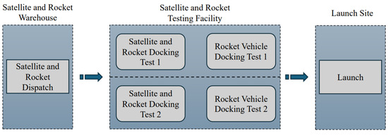
Figure 1.
Diagram of zoning and flow relationships in the satellite–rocket testing facilities.
In Figure 2, an emergency maneuver launch mission, the launch system typically consists of launch vehicles, rockets, satellites, various facilities (warehouses), and launch sites. Rockets and satellites are typically stored in the rocket and satellite storage facilities, while launch vehicles are kept in the launch vehicle storage buildings. Before the rocket launch, the satellite–rocket docking test, launch vehicle test, and rocket–vehicle docking test must be completed. Finally, the launch vehicle transports the satellite–rocket assembly to the launch site for launch.
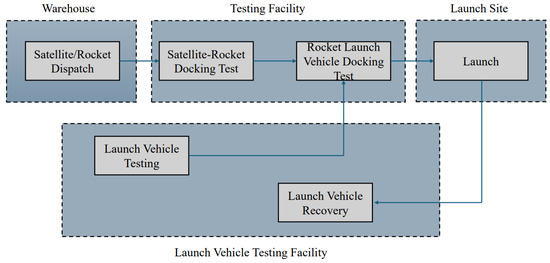
Figure 2.
Aerospace emergency launch flowchart.
The launch site consists of a standby area and a launch pad, which are located in close proximity. Prior to launch, the launch vehicle must complete vertical positioning, parameter configuration, and self-check procedures. Once these preparations are finalized, the vehicle may remain on the launch pad in a standby state for no more than 30 min. Rocket ignition and launch are treated as instantaneous events. After launch, the launch vehicle must immediately withdraw; vehicles that have not launched are not permitted to withdraw from the launch pad. In Figure 3 when multiple launch vehicles arrive simultaneously, launches must be conducted in sequence: the following vehicle must wait in the standby area until the preceding vehicle has completed its launch. Only after the prior vehicle has launched may the next vehicle enter the launch pad for final preparations. Once pre-launch procedures are completed, the launch cannot be aborted for direct withdrawal.
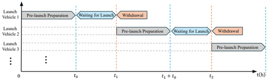
Figure 3.
Launch site multi-launch vehicle parallel scheduling timing diagram.
Prior to rocket launch, the launch vehicle undergoes a sequence of operations. It first completes testing in the launch vehicle workshop, then proceeds to the testing facility for rocket–vehicle docking tests. Subsequently, the integrated satellite–rocket assembly is transported to the launch site, where the launch is executed within the designated launch window. After the launch, the launch vehicle undergoes post-launch recovery and can be reused. The time required for each operational procedure is detailed in Table A6.
During satellite operations, some satellites function independently, while others can significantly enhance operational effectiveness through multi-satellite coordination. In certain scenarios, such coordination is indispensable to achieving mission objectives. Consequently, different launch missions contribute unequally to the formation of space capabilities—greater contribution values indicate higher significance for enhancing overall mission effectiveness. Mission contribution consists of single-mission contribution and mission group contribution. The single-mission contribution refers to the performance value obtained upon the completion of an individual launch mission. The mission group contribution refers to the additional value gained when all launch missions within a mission group are successfully completed. The total contribution of an emergency multi-mission launch plan is the sum of the single-mission contributions and the mission group contributions. More urgent emergency missions involving multi-satellite coordination can significantly enhance operational effectiveness; in some cases, such coordination is essential to achieve mission objectives. The overall mission contribution comprises both single-mission contribution and mission group contribution, as detailed in Table A7 and Table A8.
3.2. Assumptions and Related Variables
To understand the symbols and variables in the model, the following definitions and assumptions are made:
3.2.1. Assumptions
- Assume that the transportation time between facilities is calculated based on predefined distances and speeds in Table A4, without considering factors such as traffic congestion, weather, or other unforeseen delays;
- Assume that, in the absence of mission conflicts, the satellite, rocket, and launch vehicle can immediately undergo testing upon arrival at the satellite and rocket testing facility;
- Assume that the contribution of each mission is explicitly quantified in the model.
3.2.2. Related Variables
The description of variable sets and symbols used in this study is provided in Table 1.

Table 1.
Nomenclature.
4. Mixed-Integer Programming Hierarchical Collaborative Optimization (MIP-HCO) Model
The model in this study is based on the mixed-integer programming algorithm, and the bi-level collaborative optimization structure is constructed as follows.
4.1. MIP-HCO I
This paper simulates the coordinates of potential sites for constructing various types of facilities (warehouses) and launch sites, as well as the road connectivity between these sites and existing locations, as shown in Table 2. The road lengths are calculated based on the planar Euclidean distance, and a spatiotemporal location model is constructed.
Table 2.
Assume the coordinates for the distribution of emergency launch sites.
The Euclidean distance formula between two points and on a two-dimensional plane is given by
The spatiotemporal location model diagram is shown in Figure 4.
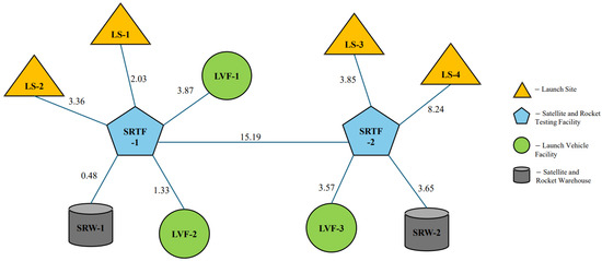
Figure 4.
Spatiotemporal location model.
4.1.1. The First-Level Objective Function
The objective of the mission is to minimize the maximum launch time of all missions, defined as the maximum value among the launch times of all missions:
where M is the set of missions and is the launch time of mission m.
4.1.2. Decision Variables
The number of satellite and rocket warehouses, satellite and rocket testing facilities, launch sites, and launch vehicles is determined based on the known conditions and assumptions:
4.1.3. Constraints
For each mission , select a launch time from its available launch time set ; for each mission , its launch time must not exceed the maximum Z launch time represented by the variable; for each mission , select a launch time from its available launch time set W; for each mission , select a testing facility from the set of satellite and rocket testing facilities A; for each mission , select a launch vehicle , and ensure that the type of the launch vehicle matches the rocket type; for each mission , select a launch site from the set of launch sites L; for each mission, it is necessary to ensure that the selected rocket type is compatible with the satellite type. The K-type rocket is compatible with A- and B-type satellites, while the Z-type rocket is compatible with A-, B-, C-, and D-type satellites; for each satellite and rocket warehouse , the total usage of rocket types K and Z cannot exceed the warehouse capacity; for each satellite and rocket warehouse , the total usage of satellite types cannot exceed the warehouse capacity; The 13 h time window for each satellite and rocket testing facility at any time t is determined by the maximum time required for satellite and rocket docking tests; a maximum of only two missions can be processed, for each mission , launch time , and satellite and rocket testing facility , the docking test and time window matching constraints.
4.1.4. Branch-and-Bound Method for Solving the First Model
Branch-and-bound is a global optimization algorithm used to solve mixed-integer programming (MIP) problems, primarily applied to optimization problems that include integer variables. The core idea is to find the optimal solution by decomposing the problem, calculating upper and lower bounds, and gradually narrowing the solution space. The specific steps are as follows:
- 1.
- Relaxation: First, ignore the integer constraints and convert the problem into a linear programming or nonlinear programming problem, allowing the variables to take non-integer values. This is referred to as the relaxed problem;
- 2.
- Branching: If the solution to the relaxed problem does not satisfy the integer constraints, branching is performed on the solution. The problem is divided into two or more subproblems;
- 3.
- Bounding: By solving the relaxed problem of each subproblem, calculate the lower and upper bounds. If the solution is an integer solution and is better than the current best solution, update the current optimal solution.;
- 4.
- Pruning: If the lower bound of a subproblem is worse than the upper bound of the current optimal solution, or if it does not have an integer solution, prune that branch. The algorithm terminates when all branches have been processed or pruned, and the difference between the upper bound of the optimal integer solution and the lower bounds of all unprocessed nodes is smaller than the set tolerance.
The results of the solution are provided in the following Table 3.
Table 3.
Utilization of launch vehicles in the spatiotemporal node model (time unit: hour).
4.2. MIP-HCO II
4.2.1. The Second-Level Optimization Objective Function
Maximize the total mission contribution, which is the sum of the contribution of individual missions and the contribution of the combined missions:
where M is the set of missions, ; is the individual contribution of mission m; C is the set of combined missions; is the additional contribution of the combined set c; if mission m is selected, ; if the combination c is implemented, .
4.2.2. New Decision Dimension Variables
denotes whether mission m is selected; if mission m is selected, ; otherwise, ; denotes whether mission group c is implemented; if mission group c is selected, ; otherwise, ;
4.2.3. Reinforce the Constraints
- 1.
- Mission Allocation Constraints:For each mission , if the mission is selected, a launch time must be chosen; each mission can only be scheduled within its specified available launch window ; for the K-type rocket, consider the dispatch time, testing time, waiting time before launch, and travel time. The launch window should be at least 18 h; Similarly, for the Z-type rocket, the launch window should be at least 14 h.
- 2.
- Resource Allocation Constraints:For each mission , denotes whether mission m is assigned to warehouse w; denotes whether mission m is assigned to the satellite–rocket warehouse a; denotes whether mission m is assigned to launch vehicle v; denotes whether mission m is assigned to launch site l.
- 3.
- Resource Capacity and Compatibility Constraints:For each warehouse m and rocket types K and Z, ensure that the total number of rockets used does not exceed the inventory available in the satellite rocket warehouse; For each warehouse w and satellite types , and D, ensure that the total number of satellites used does not exceed the inventory available in the satellite rocket warehouse; denotes whether mission m is assigned to the satellite rocket testing facility a at time t; for each satellite rocket testing facility a and time t, considering that a type-K rocket requires a total of 13 h for testing and a type-Z rocket requires a total of 11 h, the maximum duration is taken as 13 h. Therefore, within a 13 h time window from the launch time onward, at most two testing missions can be executed simultaneously at the satellite rocket testing facility a; for each launch vehicle v and time t, it can execute at most one mission at any given time. Additionally, type-K rockets are compatible with satellite types A and B, while type-Z rockets are compatible with satellite types , and D. A more detailed constraint selection flowchart is provided in Figure A1.
4.2.4. KNN and B&B Method for Solving the Second Model
The results of the solution are provided in the following Table 4.
Table 4.
Mission contribution optimization planning scheme.
5. Computational Results
5.1. Results of Model 1
By combining Equations (1)–(5) with the Algorithm 1, the shortest launch time and optimal launch planning solution for conventional launch mission planning are obtained as demonstrated in Table 3.
| Algorithm 1: MIP-HCO I |
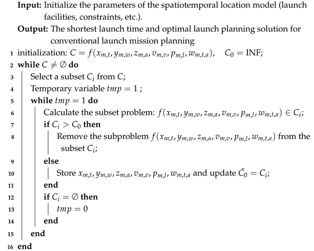 |
Figure 5 illustrates the mission time interval distributions for the two satellite–rocket test facilities (SRTF-1 and SRTF-2), which directly reflect the recovery and reusability time data of the launch vehicles presented in Table 3.
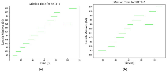
Figure 5.
The shortest launch time and optimal planning solution in MIP-HCO I: (a) Mission time interval distribution in satellite–rocket testing facility 1. (b) Mission time interval distribution in satellite–rocket testing facility 2.
- 1.
- Mission Allocation Optimization: As shown in Figure 5, the 25 missions are optimally allocated to the two test facilities:
- SRTF-1 handled a total of 13 missions: M7, M21, M9, M10, M16, M4, M24, M14, M25, M23, M6, M15, and M12.
- SRTF-2 handled a total of 12 missions: M22, M1, M18, M8, M17, M11, M20, M5, M2, M3, M13, and M19.
This allocation takes into account the recovery and reusability times of each mission, as presented in Table 3, ensuring the efficient utilization of the test facilities; - 2.
- Mission Sequencing and Time Optimization: The mission sequencing shown in Figure 5 demonstrates the intelligent scheduling based on the data presented in Table 3:
- Missions with shorter recovery times (e.g., M7 with 16.45 and M21 with 24.67) are scheduled earlier in the sequence.
- Missions with longer recovery times (e.g., M19 with 123.14 and M12 with 113.29) are scheduled towards the end of the sequence or at appropriate positions to avoid conflicts.
For example, Mission M7 begins the earliest in SRTF-1, with a recovery time of 16.45 and a reusability time of 18.95, allowing subsequent missions to follow promptly; - 3.
- Resource Conflict Avoidance Strategy: The sequencing in Figure 5 illustrates how conflicts in the use of the same launch vehicle are avoided:
- Similarly, the KLV-9 vehicle is used for three missions (M1, M14, and M17). By scheduling M1 and M17 in SRTF-2, and M14 in SRTF-1 with appropriate time intervals, resource occupation conflicts are avoided.
This cross-facility and within-facility temporal offset scheduling ensures that the use of the KLV-9 vehicle, as well as other vehicles, does not result in conflicts.
5.2. Evaluation of Overall Time Utilization Efficiency in Model 1 Minimization
From the computed Mission Table 3, it is evident that the majority of the satellite launch mission time is allocated to satellite and rocket docking tests and rocket–vehicle docking tests, both conducted at the satellite and rocket testing facility. Therefore, to assess overall resource utilization efficiency, we evaluate the utilization of the satellite and rocket testing facility during the time span from the initiation of the first mission to the completion of the final mission.
Overall Time Calculation: the total time is defined as the time interval from the start of the first mission to the completion of the last mission.
where represents the maximum value among all mission completion times, and represents the minimum value among all mission start times.
Proportion of Time with at Least One Mission in Testing: define as the total time during which at least one mission is undergoing testing. This is determined by discretizing the time interval, based on the time step , and checking at each time point whether a mission is in progress. If at least one mission is being tested during a given time interval, that interval is counted towards .
where denotes the number of missions being executed at time t.
The percentage of time during which at least one mission is in testing relative to the total time is
The proportion of time during which two missions are simultaneously in testing is calculated as follows: define as the total time during which two or more missions are simultaneously in testing. The method is similar: each time interval is checked, and if at least two missions are in testing, that interval is counted towards .
The percentage of time during which two missions are simultaneously in testing relative to the total time is
After calculation, satellite rocket testing facility 1 had at least one mission in testing for of the total time, while the percentage of time with two simultaneous missions in testing was ; Similarly, satellite rocket testing facility 2 had at least one mission in testing for of the total time, while the percentage of time with two simultaneous missions in testing was .
5.3. Results of Model 2
By combining Equations (6)–(10) with the Algorithm 2, under more time-constrained conditions, the maximum contribution includes 16 missions, achieving a contribution value of 166.5.
| Algorithm 2: MIP-HCO II |
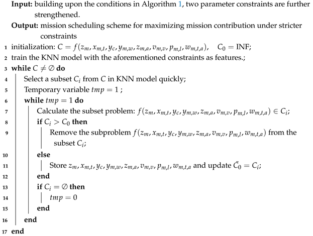 |
The conflict analysis of satellite and rocket testing facility utilization in the planning scheme indicates that this set of planning schemes shows no conflicts in the utilization of the facilities. Figure 6 represents the optimal result obtained from our simulation.
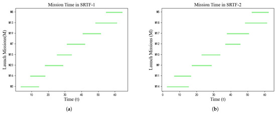
Figure 6.
The shortest launch time and optimal planning solution in MIP-HCO II: (a) Mission time interval distribution in satellite–rocket testing facility 1. (b) Mission time interval distribution in satellite–rocket testing facility 2.
Figure 7 illustrates the emergency launch decision diagram under the second mission contribution model.
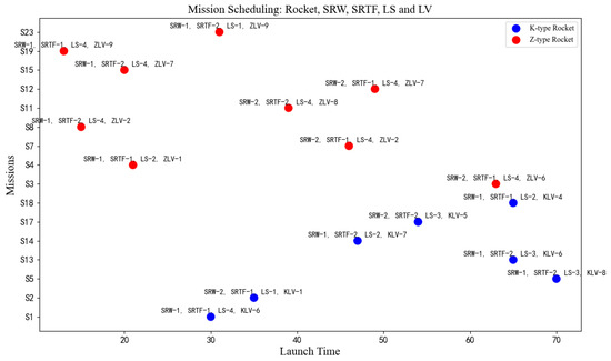
Figure 7.
Decision results of Model 2.
5.4. Evaluation of Overall Time Utilization Efficiency in MIP-HCO II Minimization
Using a similar approach based on Equations (11)–(15), the resource utilization of the satellite rocket testing facility is calculated under stricter constraints.
For testing facility 1, at least one mission was in testing for 100% of the total time, while the percentage of time with two simultaneous missions in testing was 42.86%.
For testing facility 2, at least one mission was in testing for 97.05% of the total time, while the percentage of time with two simultaneous missions in testing was 59.30%.
6. Model Comparison Experiment
To evaluate the effectiveness of the proposed MIP-HCO model integrated with KNN+B&B, a systematic comparative analysis was conducted against widely-used heuristic algorithms, including the Simulated Annealing (SA) algorithm, Ant Colony Optimization (ACO) algorithm, and Genetic Algorithm (GA).
6.1. Modeling of Comparative Experiments (Using Simulated Annealing as an Example)
In 1993, Bertsimas et al. [31] proposed the Simulated Annealing (SA) algorithm, which is a type of heuristic intelligent optimization algorithm. The design inspiration for the SA algorithm originates from the annealing process in physics, where metal is slowly cooled to reach its lowest energy state, forming a stable crystalline structure. When solving optimization problems, the Simulated Annealing algorithm mimics this process to find the global optimal solution in a complex solution space. During the search process, SA gradually lowers the temperature to control exploration. In the high-temperature phase, the algorithm allows the acceptance of inferior solutions to increase solution diversity and prevent getting trapped in local optima. As the temperature decreases, the algorithm gradually reduces the probability of accepting worse solutions, converging towards a better solution, and eventually reaching the global optimum. The SA strategy is to explore a broad solution space by randomly accepting inferior solutions and then gradually narrowing the search range as the temperature decreases, thereby concentrating solutions around the optimal solution.
In this study, the algorithm consists of the following core components:
- 1.
- Temperature Check: Verify whether the current temperature is greater than zero. If the temperature has dropped to zero, the iteration terminates, and the final result is output. Otherwise, the iteration continues;
- 2.
- Generation of Neighborhood Solution: Randomly perturb decision variables such as mission assignments, launch timing, satellite–rocket storage facilities, satellite–rocket testing facilities, launch sites, and launch vehicles. The operator represents a randomly selected operation from the given set.
- 3.
- Penalty Calculation: The penalty term is computed as defined below, where represents the penalty weights associated with different constraints; and represent the inventory of K-type and Z-type rockets in storage facility w, respectively; represents the inventory of satellite type s in storage facility w; is the compatibility function between rocket and launch vehicle , where it equals 1 if they are incompatible, and it equals 0 if they are compatible.
- 4.
- Compute the difference between the contribution of the neighborhood solution and the penalty term. The contribution of each mission and mission group in the neighborhood solution is calculated using the objective function, and the penalty term is then subtracted.
- 5.
- Decision to Accept the Neighborhood Solution: Compare the difference between the current solution and the new solution in terms of contribution minus the penalty term. If the new solution yields a higher contribution than the current solution, it is accepted. Otherwise, acceptance is determined probabilistically using an acceptance probability formula. p represents the probability of accepting the new solution; represents the difference between the contribution of the current solution and the penalty term; represents the contribution of the current solution.
6.2. Comparison of SA Results
From Figure 8, the red curve (KNN + B&B) demonstrates a faster convergence, reaching 166.5 within approximately 3500 iterations. In contrast, the blue curve (SA) requires around 9000 iterations to attain a 163.5 value.
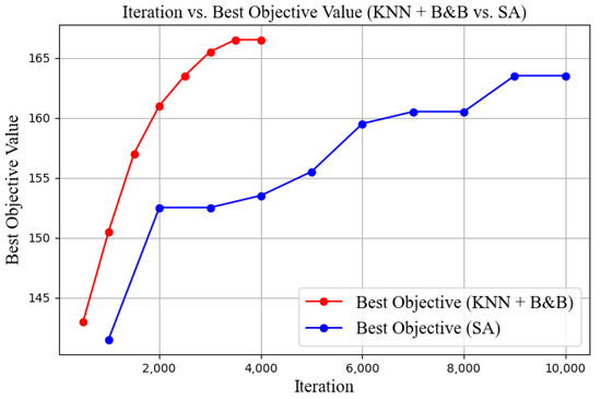
Figure 8.
Comparison chart of iteration count and optimal value (KNN+B&B vs. SA).
From Figure 9, KNN + B&B requires only 9.5 s, whereas SA takes 40.18 s, reducing computation time by nearly 76.35%.
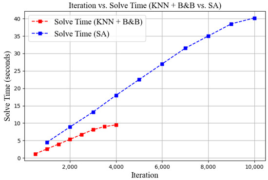
Figure 9.
Comparison of iteration count and solution time (KNN+B&B vs. SA).
6.3. Comparison of ACO Results
Following the methodology outlined in Section 6.1, a comparative analysis between KNN+B&B and ACO (Appendix D and Figure A2) was conducted, with the results summarized as follows.
From Figure 10, the red curve (KNN + B&B) demonstrates a faster convergence, reaching 166.5 within approximately 3500 iterations. In contrast, the origin curve (ACO) requires around 3000 iterations to attain an optimal value of 162.
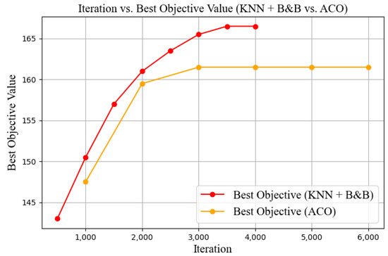
Figure 10.
Comparison chart of iteration count and optimal value (KNN+B&B vs. ACO).
From Figure 11, KNN + B&B required only 9.5 s, whereas ACO took 19.5 s, reducing computation time by nearly 51.28%.
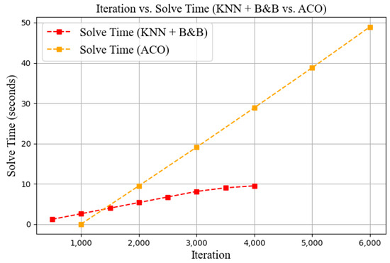
Figure 11.
Comparison of iteration count and solution time (KNN+B&B vs. ACO).
6.4. Comparison of GA Results
Following the methodology outlined in Section 6.1, a comparative analysis between KNN+B&B and GA (Appendix E and Figure A3) was conducted, with the results summarized as follows.
From Figure 12, the red curve (KNN + B&B) demonstrates a faster convergence, reaching 166.5 within approximately 3500 iterations. In contrast, the green curve (GA) requires around 6000 iterations to attain an optimal value of 160.
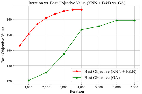
Figure 12.
Comparison chart of iteration count and optimal value (KNN+B&B vs. GA).
From Figure 13, KNN + B&B required only 9.5 s, whereas GA took 27 s, reducing computation time by nearly 64.81%.
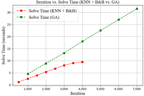
Figure 13.
Comparison of iteration count and solution time (KNN+B&B vs. GA).
6.5. Comprehensive Evaluation
Table 5 indicates that the KNN + B&B algorithm achieves the best performance, reaching the optimal contribution value of 166.5 with only 3500 iterations and a solving time of 9.5 s. It outperforms other algorithms (SA, ACO, GA) in both efficiency and solution quality.
Table 5.
Results of Algorithmic Comparison.
7. Model Expansion
7.1. KNN+B&B Computational Complexity Analysis
7.1.1. KNN Complexity Analysis
- KNN training phase: , where m is the number of training samples and d is the feature dimension;
- KNN accelerated selection phase: , where k is the number of neighbors.
7.1.2. B&B Complexity Analysis
- B&B phase: , where V denotes the number of binary variables;
- In the MIP-HCO model, the number of binary variables V is given bywhere n denotes the number of missions; |LW|, |SRW|, |SRTF|, |LV|, and |LS| represent the cardinalities of the sets of launch windows, satellite–rocket warehouse, satellite–rocket test facilities, launch vehicles, and launch sites, respectively; and |Contribution| represents the size of the contribution relation set between missions.
7.1.3. KNN + B&B Complexity Analysis
By integrating Section 7.1.1 and Section 7.1.2, the reduced total computational complexity of the KNN + B&B algorithm is .
Figure 14 illustrates a simulated complexity analysis curve of the algorithm throughout its solution process.
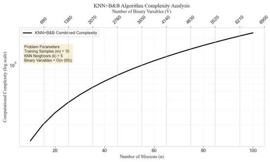
Figure 14.
Complexity analysis curve for the KNN+B&B algorithm.
Figure 14 illustrates the computational complexity trend of the KNN + B&B algorithm as the problem size increases. As the number of missions (n) grows from 10 to 100, the computational complexity exhibits a clear nonlinear increase, forming a convex curve under the logarithmic scale.
7.2. Scalability Analysis for Expanded Problem Sizes
As shown in Figure 15, a systematic analysis was conducted on the time complexity variation of the KNN + B&B algorithm under dual constraints, by simultaneously increasing the number of missions and launch windows.
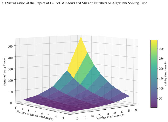
Figure 15.
Effects of mission scale and launch window count on algorithm performance.
Figure 15 illustrates the combined impact of the number of launch windows (w) and the number of missions (n) on the algorithm’s solving time. As both parameters increase, the solving time exhibits a clear nonlinear growth trend. The color gradient—from purple (<50 s) to yellow (>300 s)—visually highlights the significant variation in computational complexity. When either n is fixed and w increases, or w is fixed and n increases, the observed growth in solving time aligns with the theoretical time complexity discussed in Section 7.1.3. This dual-parameter influence mechanism indicates that the computational complexity of the algorithm is jointly governed by the polynomial term (reflecting mission scale) and the exponential term (reflecting the combinatorial effect of launch windows).
8. Discussion
The results of this study demonstrate that the MIP-HCO model, when combined with the KNN + B&B optimization strategy, significantly enhances scheduling efficiency for launch missions under constrained time and resource conditions. Compared to traditional integer programming methods, the proposed approach exhibits notable advantages in terms of computational complexity and solution speed. These findings align with existing research on scheduling optimization, which emphasizes the potential of heuristic search combined with machine learning techniques for improving computational efficiency. However, traditional heuristic approaches often suffer from local optima traps when dealing with complex constraints. By introducing KNN-based approximate evaluation, this study effectively reduces the computational burden of the Branch and Bound (B&B) method, thereby improving solution speed while ensuring global optimality. Moreover, the results indicate that, under mission contribution optimization constraints, applying an integer programming-based re-optimization strategy further enhances mission execution efficiency. Compared to traditional fixed-priority scheduling methods, the proposed approach dynamically selects high-value mission combinations, effectively adapting to varying mission requirements. This method has broad applicability for rapid response in aerospace emergency missions, particularly in scenarios with limited resources or constrained launch windows, where its optimization capabilities are especially pronounced. Nevertheless, certain limitations remain in this study. First, the accuracy of KNN-based approximate evaluation depends on the representativeness of the training data. Consequently, when facing different types of mission demands, the KNN model parameters may require adjustment to adapt to new mission environments. Second, the integer programming optimization strategy employed in this study is tailored to the current scheduling environment; future research could explore reinforcement learning (RL) or deep reinforcement learning (DRL) techniques to enable continuous optimization in dynamically evolving environments. Additionally, in more complex aerospace mission scenarios—such as those involving multiple launch platforms or intricate mission dependencies—further investigation is required to extend the applicability of the current approach.
9. Conclusions
This study proposes the MIP-HCO model to optimize the scheduling and execution of emergency launch missions, integrating KNN + B&B to enhance computational efficiency and global optimality. Experimental results demonstrate that this approach optimizes mission scheduling, reduces execution time, improves resource utilization, and enhances system adaptability, providing efficient support for aerospace emergency decision-making.
Author Contributions
Conceptualization, F.Z. and Y.C.; methodology, F.Z. and Y.C.; software, X.L., F.Z. and J.H.; validation, X.L. and F.Z.; formal analysis, F.Z. and Y.C.; investigation, F.Z. and Y.C.; resources, F.Z. and Y.C.; data curation, F.Z. and Y.C.; writing—original draft preparation, X.L.; writing—review and editing, X.L.; visualization, X.L. and J.H.; supervision, F.Z. and Y.C.; project administration, X.L. and Y.C.; funding acquisition, Y.C. All authors have read and agreed to the published version of the manuscript.
Funding
This research was funded by the National Natural Science Foundation of China (No. 72461001), and the Guangxi Natural Science Foundation (No. 2025GXNSFAA069957).
Data Availability Statement
The original contributions presented in the study are included in the article; further inquiries can be directed to the corresponding author.
Acknowledgments
Xiangzhe Li thanks Feng Zhan and Yan Chen for the helpful guide. Finally, the authors thank the reviewers and the editor’s office for their supportive help.
Conflicts of Interest
The authors declare no conflicts of interest.
Appendix A. The Details of the Problem Description
Table A1.
Inventory status of satellite and rocket storage facilities.
Table A1.
Inventory status of satellite and rocket storage facilities.
| Serial Number | Satellite and Rocket Warehouse | K-Type Rocket | Z-Type Rocket | A-Type Satellite | B-Type Satellite | C-Type Satellite | D-Type Satellite |
|---|---|---|---|---|---|---|---|
| 1 | SRW-1 | 12 | 13 | 7 | 10 | 5 | 8 |
| 2 | SRW-2 | 18 | 7 | 8 | 5 | 10 | 7 |
Table A2.
Satellite and rocket model compatibility.
Table A2.
Satellite and rocket model compatibility.
| Serial Number | Rocket | Compatible Satellite |
|---|---|---|
| 1 | K-type Rocket | A,B |
| 2 | Z-type Rocket | A,B,C,D |
Table A3.
Simulation mission checklist (launch windows * unit: h).
Table A3.
Simulation mission checklist (launch windows * unit: h).
| Mission | X-Type Satellite | Launch Window A | Launch Window B | Launch Window C |
|---|---|---|---|---|
| M1 | D | 15 | 28 | 45 |
| M2 | B | 22 | 32 | 57 |
| M3 | C | 17 | 44 | 65 |
| M4 | A | 20 | 30 | 51 |
| M5 | A | 18 | 31 | 72 |
| M6 | B | 15 | 37 | 53 |
| M7 | C | 17 | 46 | 49 |
| M8 | D | 14 | 40 | 52 |
| M9 | D | 15 | 43 | 67 |
| M10 | B | 17 | 38 | 53 |
| M11 | C | 19 | 39 | 59 |
| M12 | A | 13 | 40 | 45 |
| M13 | A | 20 | 37 | 59 |
| M14 | B | 19 | 35 | 60 |
| M15 | C | 20 | 36 | 54 |
| M16 | D | 22 | 35 | 57 |
| M17 | D | 19 | 25 | 54 |
| M18 | B | 24 | 40 | 66 |
| M19 | C | 20 | 42 | 55 |
| M20 | A | 13 | 26 | 57 |
| M21 | A | 15 | 29 | 65 |
| M22 | B | 13 | 16 | 58 |
| M23 | C | 20 | 33 | 53 |
| M24 | D | 14 | 38 | 62 |
| M25 | D | 17 | 44 | 54 |
* The launch windows represent the earliest permissible time for rocket launch relative to the reference time, referred to as the leading edge of the window.
Table A4.
Predefined speeds table (unit: km/h).
Table A4.
Predefined speeds table (unit: km/h).
| K-Type Launch Vehicle Speed | Z-Type Launch Vehicle Speed | No-Load Speed * |
|---|---|---|
| 35 | 25 | 50 |
* Under no-load conditions, both types of launch vehicles exhibit a travel speed of 50 km/h.
Table A5.
Assigned launch vehicle identification numbers for each launch vehicle facility.
Table A5.
Assigned launch vehicle identification numbers for each launch vehicle facility.
| Serial Number | Launch Vehicle Facility | K-Type Launch Vehicle | Z-Type Launch Vehicle |
|---|---|---|---|
| 1 | LVF-1 | KLV-1, KLV-2, KLV-3 | ZLV-1, ZLV-2, ZLV-3 |
| 2 | LVF-2 | KLV-4, KLV-5, KLV-6 | ZLV-4, ZLV-5, ZLV-6 |
| 3 | LVF-3 | KLV-7, KLV-8, KLV-9 | ZLV-7, ZLV-8, ZLV-9 |
Table A6.
Time consumption for each process (unit: hours).
Table A6.
Time consumption for each process (unit: hours).
| Rocket | Satellite and Rocket Docking Test | Rocket–Vehicle Docking Test | Launch Vehicle Test | Pre-Launch Preparation | Awaiting Launch | Launch Vehicle Withdrawal | Post-Launch Recovery of Launch Vehicle |
|---|---|---|---|---|---|---|---|
| K-type | 12 | 1 | 0.5 | 3 | 0.25 | 1.5 | |
| Z-type | 10 | 1 | 0.5 | 1 | 0.33 | 2.5 |
Appendix B. Mission Contribution in the MIP-HCO II Model
Table A7.
Single-mission contribution.
Table A7.
Single-mission contribution.
| Mission | Contribution | Mission | Contribution |
|---|---|---|---|
| M1 | 1.5 | M14 | 2 |
| M2 | 2 | M15 | 2.5 |
| M3 | 6 | M16 | 4 |
| M4 | 3 | M17 | 12 |
| M5 | 8 | M18 | 7 |
| M5 | 5 | M19 | 2 |
| M7 | 4 | M20 | 2 |
| M8 | 3 | M21 | 3 |
| M9 | 1 | M22 | 5 |
| M10 | 6 | M23 | 4 |
| M11 | 1.5 | M24 | 2 |
| M12 | 2.5 | M25 | 3 |
| M13 | 1.5 | — | — |
Table A8.
Mission group contribution degree.
Table A8.
Mission group contribution degree.
| Serial Number | Mission Group | Mission Group Contribution | Serial Number | Mission Group | Mission Group Contribution |
|---|---|---|---|---|---|
| M1, M2 | 2 | M11, M14, M15 | 6 | ||
| M4, M5 | 4 | M12, M14, M15 | 6 | ||
| M3, M7, M8 | 5 | M11, M12, M14 | 7 | ||
| M9, M10 | 5 | M11, M12, M15 | 7 | ||
| M11, M12, M13 | 6 | M11, M13, M14 | 8 | ||
| M12, M13, M14 | 7 | M16, M19, M23 | 9 | ||
| M13, M14, M15 | 8 | M21, M24, M25 | 9 | ||
| M11, M12, M13, M14 | 9 | M6, M8, M20, M22 | 9 | ||
| M12, M13, M14, M15 | 9 | M11, M12, M13, M15 | 10 | ||
| M11, M13, M14, M15 | 10 | M11, M12, M13, M14, M15 | 11 |
Appendix C. The Details of Selection Process Under Multiple Constraints
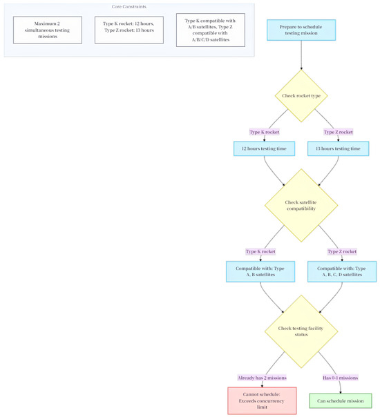
Figure A1.
Dynamic selection process under multiple constraints.
Appendix D. The Details of Modeling of Comparative Experiment (ACO)
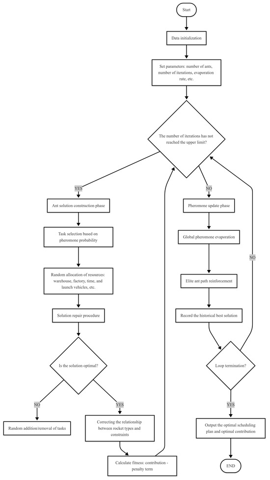
Figure A2.
Comparison model experiment ACO algorithm flowchart.
Appendix E. The Details of Modeling of Comparative Experiment (GA)
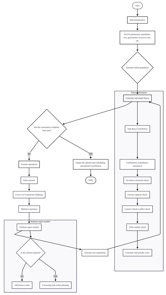
Figure A3.
Comparison model experiment GA algorithm flowchart.
References
- Matteo, M.; Molinaro, A.; Morosi, S.; Scalise, S. Aerospace Communications for Emergency Applications. Proc. IEEE 2011, 99, 1267–1284. [Google Scholar] [CrossRef]
- Wu, F.; Liu, X.; Wang, J.; Li, C.; Liu, Y.; Su, J.; Zhang, A.; Wang, M. Research on agile space emergency launching mission planning simulation and verification method. J. Syst. Eng. Electron. 2023, 34, 1023–1045. [Google Scholar]
- Duan, J.; Liu, Y. Two-dimensional launch window method to search for launch opportunities of interplanetary missions. Chin. J. Aeronaut. 2020, 11, 739–749. [Google Scholar] [CrossRef]
- Dai, C.-Q.; Zhang, Y.; Yu, F.R.; Chen, Q. Dynamic scheduling scheme with mission laxity for data relay satellite networks. IEEE Trans. Veh. Technol. 2024, 73, 2605–2620. [Google Scholar] [CrossRef]
- Wang, Y.; Liu, J.; Yin, Y.; Tong, Y.; Liu, J. Space information network resource scheduling for cloud computing: A deep reinforcement learning approach. Wirel. Commun. Mob. Comput. 2022, 1, 1927937. [Google Scholar] [CrossRef]
- Meng, S.; Xing, L.; Levitin, G. Activation delay and aborting policy minimizing expected losses in consecutive attempts having cumulative effect on mission success. Reliab. Eng. Syst. Saf. 2024, 247, 110078. [Google Scholar] [CrossRef]
- Qiu, Q.; Cui, L. Gamma process based optimal mission abort policy. Reliab. Eng. Syst. Saf. 2019, 190, 106496. [Google Scholar] [CrossRef]
- Li, C.; Chen, H.; Xiahou, T.; Zhang, Q.; Liu, Y. Health status assessment of radar systems at aerospace launch sites by fuzzy analytic hierarchy process. Qual. Reliab. Eng. Int. 2023, 39, 3385–3409. [Google Scholar] [CrossRef]
- Resende, B.A.D.; Dedini, F.G.; Eckert, J.J.; Sigahi, T.F.; Pinto, J.D.S.; Anholon, R. Proposal of a facilitating methodology for fuzzy FMEA implementation with application in process risk analysis in the aeronautical sector. Int. J. Qual. Reliab. Manag. 2024, 41, 1063–1088. [Google Scholar] [CrossRef]
- Huang, T.; Xiahou, T.; Mi, J.; Chen, H.; Huang, H.Z.; Liu, Y. Merging multi-level evidential observations for dynamic reliability assessment of hierarchical multi-state systems: A dynamic Bayesian network approach. Reliab. Eng. Syst. Saf. 2024, 249, 110225. [Google Scholar] [CrossRef]
- Wang, X.; Liang, X.D.; Li, X.Y.; Luo, P. An Integrated Multiattribute Group Decision-Making Approach for Risk Assessment in Aviation Emergency Rescue. Int. J. Aerosp. Eng. 2022, 1, 9713921. [Google Scholar] [CrossRef]
- Kaplan, M.H. Modern Satellite Dynamics and Control; Courier Dover Publications: New York, NY, USA, 2020; pp. 1–432. Available online: https://books.google.co.jp/books?hl=en&lr=&id=aF0EEAAAQBAJ&oi=fnd&pg=PA1&dq=Modern+Satellite+Dynamics+and+Control&ots=qTg4W-zsbf&sig=jPhiHBFv22xb4tR9CrNsIsyxHNI&redir_esc=y#v=onepage&q=Modern%20Satellite%20Dynamics%20and%20Control&f=false (accessed on 18 November 2020).
- Houin, A.; Sood, R. Optimal launch windows for artemis iii and beyond leveraging contour maps. In Proceedings of the 73rd International Astronautical Congress (IAC), Paris, France, 18–22 September 2022. Available online: https://www.researchgate.net/profile/Aaron-Houin/publication/364829121_Optimal_Launch_Windows_for_Artemis_III_and_Beyond_Leveraging_Contour_Maps/links/65de0b1aadf2362b635a6606/Optimal-Launch-Windows-for-Artemis-III-and-Beyond-Leveraging-Contour-Maps.pdf (accessed on 23 September 2022).
- Brandimarte, P. Scheduling satellite launch missions: An MILP approach. J. Sched. 2013, 16, 29–45. [Google Scholar] [CrossRef]
- Zhaojun, Z.; Funian, H.; Yanhua, Y.; Na, Z. Ant colony algorithm for satellite control resource scheduling problem. Artif. Intell. 2018, 48, 3295–3305. [Google Scholar]
- Wang, Y.; Sheng, M.; Zhuang, W.; Zhang, S.; Zhang, N.; Liu, R.; Li, J. Multi-resource coordinate scheduling for earth observation in space information networks. IEEE J. Sel. Areas Commun. 2018, 36, 268–279. [Google Scholar] [CrossRef]
- Chen, L.; Tang, F.; Li, Z.; Yang, L.T.; Yu, J.; Yao, B. Time-varying resource graph based resource model for space-terrestrial integrated networks. In Proceedings of the IEEE INFOCOM 2021-IEEE Conference on Computer Communications, Vancouver, BC, Canada, 10–13 May 2021; pp. 1–10. [Google Scholar] [CrossRef]
- Cui, J.; Zhang, X. Application of a multi-satellite dynamic mission scheduling model based on mission priority in emergency response. Sensors 2019, 19, 1430. [Google Scholar] [CrossRef]
- Yi, G.; Chao, H.; Yunhan, C.; Wei, X.W. Mission replanning for multiple agile earth observation satellites based on cloud coverage forecasting. IEEE J. Sel. Top. Appl. Earth Obs. Remote Sens. 2021, 15, 594–608. Available online: https://ieeexplore.ieee.org/stamp/stamp.jsp?arnumber=9652077 (accessed on 15 December 2021).
- Zhuo, H.H.; Kambhampati, S. Model-lite planning: Case-based vs. model-based approaches. Artif. Intell. 2017, 246, 1–21. [Google Scholar] [CrossRef]
- Haslum, P.; Ivankovic, F.; Ramirez, M.; Gordon, D.; Thiébaux, S.; Shivashankar, V.; Nau, D. Extending classical planning with state constraints: Heuristics and search for optimal planning. J. Artif. Intell. Res. 2018, 62, 373–431. [Google Scholar] [CrossRef]
- Soleymani, M.; Fakoor, M.; Bakhtiari, M. Optimal mission planning of the reconfiguration process of satellite constellations through orbital maneuvers: A novel technical framework. Adv. Space Res. 2019, 63, 3369–3384. [Google Scholar] [CrossRef]
- Fakoor, M.; Bakhtiari, M.; Soleymani, M. Optimal design of the satellite constellation arrangement reconfiguration process. Adv. Space Res. 2016, 58, 372–386. [Google Scholar] [CrossRef]
- Niu, C.; Li, A.; Huang, X.; Li, W.; Xu, C. Research on global dynamic path planning method based on improved A* algorithm. Math. Probl. Eng. 2021, 2021, 4977041. [Google Scholar] [CrossRef]
- Morgado, F.M.P.; Marta, A.C.; Gil, P.J.S. Multistage rocket preliminary design and trajectory optimization using a multidisciplinary approach. Struct. Multidiscip. Optim. 2022, 65, 192. [Google Scholar] [CrossRef]
- Benedikter, B.; Zavoli, A.; Colasurdo, G.; Pizzurro, S.; Cavallini, E. Convex approach to three-dimensional launch vehicle ascent trajectory optimization. Journal of Guidance, Control, and Dynamics. J. Guid. Control Dyn. 2021, 44, 1116–1131. [Google Scholar] [CrossRef]
- Federici, L.; Zavoli, A.; Colasurdo, G.; Mancini, L.; Neri, A. Integrated optimization of first-stage SRM and ascent trajectory of multistage launch vehicles. J. Spacecr. Rockets. 2021, 58, 786–797. [Google Scholar] [CrossRef]
- Mahjub, A.; Mazlan, N.M.; Abdullah, M.Z.; Azam, Q. Design optimization of solid rocket propulsion: A survey of recent advancements. J. Spacecr. Rockets. 2020, 57, 3–11. [Google Scholar] [CrossRef]
- Chen, H.; Sarton du Jonchay, T.; Hou, L.; Ho, K. Multifidelity space mission planning and infrastructure design framework for space resource logistics. J. Spacecr. Rockets. 2021, 58, 538–551. [Google Scholar] [CrossRef]
- Gollins, N.; Ho, K. Hierarchical Framework for Space Exploration Campaign Schedule Optimization. J. Spacecr. Rockets. 2024, 61, 1146–1164. [Google Scholar] [CrossRef]
- Bertsimas, D.; Tsitsiklis, J. Simulated annealing. Stat. Sci. 1993, 8, 10–15. [Google Scholar] [CrossRef]
- Chen, Z.; Wang, R.L. Ant colony optimization with different crossover schemes for global optimization. Cluster Comput 2017, 20, 1247–1257. [Google Scholar] [CrossRef]
- Kordos, M.; Boryczko, J.; Blachnik, M.; Golak, S. Optimization of Warehouse Operations with Genetic Algorithms. Appl. Sci. 2020, 10, 4817. [Google Scholar] [CrossRef]
Disclaimer/Publisher’s Note: The statements, opinions and data contained in all publications are solely those of the individual author(s) and contributor(s) and not of MDPI and/or the editor(s). MDPI and/or the editor(s) disclaim responsibility for any injury to people or property resulting from any ideas, methods, instructions or products referred to in the content. |
© 2025 by the authors. Licensee MDPI, Basel, Switzerland. This article is an open access article distributed under the terms and conditions of the Creative Commons Attribution (CC BY) license (https://creativecommons.org/licenses/by/4.0/).