Energy-Adaptive SGHSMC: A Particle-Efficient Nonlinear Filter for High-Maneuver Target Tracking

Abstract

Tracking targets with nonlinear motion patterns remains a significant challenge in state estimation. We propose an energy-adaptive stochastic gradient Hamiltonian sequential Monte Carlo (SGHSMC) filter that combines adaptive energy dynamics with efficient particle sampling. The proposed method features a novel energy function that automatically adapts to target dynamics while minimizing the need for resampling operations. By integrating Hamiltonian Monte Carlo sampling with stochastic gradient techniques, our approach achieves a 40% reduction in computational overhead compared to traditional particle filters while maintaining particle diversity. We validate the method through both simulation and experimental studies. The simulation employs a univariate nonstationary growth model, demonstrating improvements of 39% in tracking accuracy over the extended Kalman filter (EKF) and 29% over standard sequential Monte Carlo methods. The experimental validation uses a bearing-only tracking scenario with a quadrupedal robot executing complex maneuvers, tracked by high-precision angular measurement systems. In practical tracking scenarios, the SGHSMC filter achieves a 77% better accuracy than EKF while maintaining the computational efficiency suitable for real-time applications. The algorithm demonstrates effectiveness in scenarios involving rapid state changes and irregular motion patterns, offering a robust solution for challenging target tracking problems.

1. Introduction

The tracking of targets exhibiting highly nonlinear and irregular motion patterns presents significant challenges in various applications, from autonomous navigation to robotic systems [1,2]. These targets often demonstrate complex dynamics characterized by sudden accelerations, sharp directional changes, and unpredictable trajectory variations. Traditional tracking algorithms frequently struggle to maintain accuracy when confronted with such challenging scenarios, particularly when real-time performance is required.

Conventional nonlinear filtering approaches, such as the extended Kalman filter (EKF) and unscented Kalman filter (UKF), have served as standard solutions for target tracking [3]. However, these methods often fail to adequately capture complex target dynamics, especially during rapid maneuvers or when dealing with highly nonlinear measurement models. Their inherent linearization assumptions and Gaussian approximations become particularly problematic in scenarios involving irregular motion patterns.

Recent developments in particle-based methods [4,5] have shown promising results in addressing these challenges. The invariant particle filter (IPF) [6] leverages geometric structures and system symmetries to enhance stability and convergence properties in state estimation. Similarly, the particle flow filter (PFF) [7] introduces an innovative continuous time approach that transports particles from prior to posterior distributions without traditional resampling steps. However, these methods still face limitations in balancing computational efficiency with sampling accuracy, particularly when tracking targets with rapidly changing dynamics. α-stable filtering structures [8] provide robust solutions for systems affected by impulsive noise and outliers, significantly improving tracking stability in non-Gaussian environments. Progressive transform-based Gaussian particle filtering [9] offers reliable state estimation for nonlinear systems with heavy-tailed measurement noise. Soft-constrained Gaussian Process Regression [10] enhances prediction accuracy by incorporating partial system knowledge as a flexible constraint. Bayesian inference methods for zero-modified power series models [11] enable the effective statistical analysis of count data with excess zeros, commonly encountered in sparse tracking scenarios.

The Hamiltonian Monte Carlo (HMC) framework offers an alternative approach through deterministic particle dynamics [12,13,14]. The theoretical foundations of the HMC framework in filtering problems [12], along with advanced proposal distribution techniques [13] and convergence analysis [14], have established their effectiveness in high-dimensional state estimation. While the HMC framework demonstrates superior mixing properties compared to random-walk proposals, its computational requirements for exact gradient calculations often make it impractical for real-time applications. Stochastic gradient variants [15,16] attempt to address this limitation, but can struggle with maintaining the sample quality in sequential estimation contexts.

This paper introduces the stochastic gradient Hamiltonian sequential Monte Carlo (SGHSMC) filter, which combines the efficient state space exploration of the HMC framework with the computational advantages of stochastic gradient techniques.

Our approach features an adaptive energy function that automatically adjusts to target dynamics, enabling robust tracking performance while maintaining computational feasibility. Unlike existing methods that sacrifice either accuracy or speed, the SGHSMC filter achieves a balanced trade-off through its novel integration framework. By embedding stochastic gradient Hamiltonian dynamics within the sequential Monte Carlo (SMC) structure, the algorithm significantly reduces the computational overhead while preserving particle diversity. The method’s adaptive energy function dynamically responds to target maneuvers, incorporating both geometric constraints and measurement uncertainties for enhanced stability. This design, combined with a computationally efficient sampling strategy, maintains high-quality state estimation in high-dimensional spaces, supported by theoretical convergence guarantees under practical conditions.

We validate our approach through both simulation and experimental studies. The simulation employs a univariate nonstationary growth model (UNGM), which presents significant challenges for conventional filtering methods due to its strong nonlinearity and bimodal characteristics. The performance evaluation consists of two distinct scenarios: a simulation study with the UNGM and a range-bearing tracking implementation. First, a traditional UNGM to demonstrate the fundamental filtering capabilities. Second, a more practical single-target tracking scenario using range and bearing measurements from a fixed observation point. This second scenario presents significant challenges due to the nonlinear measurement model and varying target dynamics. In addition, the experimental validation uses a spiral trajectory to specifically examine the filter convergence properties and tracking performance across different filtering approaches. These validation scenarios demonstrate the SGHSMC filter’s capability to maintain accurate tracking performance while achieving a computational efficiency suitable for real-time applications.

The simulation and experimental scenarios are specifically designed to evaluate both traditional performance metrics and convergence characteristics. The rectangular trajectory provides insights into general tracking performance across different filters (EKF, UKF, SMC, HMC, SGHSMC, IPF, and PFF), while the spiral trajectory specifically challenges the convergence properties and adaptation capabilities of each approach. The results show that the SGHSMC filter achieves superior tracking accuracy compared to the existing methods, while maintaining a computational efficiency suitable for real-time applications.

The remainder of this paper is organized as follows. Section 2 presents the theoretical framework of the proposed SGHSMC filter, including the adaptive energy function design and convergence analysis. Section 3 describes the simulation and experimental studies, providing comprehensive performance comparisons with existing methods. Finally, Section 4 concludes the paper with a discussion of the results and potential future directions.

2. Stochastic Gradient Hamiltonian Sequential Monte Carlo (SGHSMC) Filter

2.1. Overview of HMC and SGHMC Integration

The HMC [12,13] sampling method provides an algorithm for defining long-range proposals with high acceptance probabilities using the Metropolis–Hasting method, which is the representative method of Markov chain Monte Carlo (MCMC), enabling a more efficient retrieval of the state space than standard random walk proposals. However, a limitation of the HMC framework is the need to compute the gradient of the potential energy function to simulate the Hamiltonian dynamics. In this paper, we propose a filter for estimating the state variable by combining the state space retrieval efficiency of the HMC framework with the big data calculation efficiency of the stochastic gradient to deal with the limitation of the HMC framework. This paper shows the implications of implementing the HMC framework using stochastic gradients, and we propose stronger Hamiltonian deformation, including noise introduced by stochastic gradient estimates. The proposed filter is called SGHSMC.

The key innovation lies in replacing the conventional resampling step of the SMC filter with SGHMC-based sampling, which provides the main benefits: the more efficient exploration of the state space through Hamiltonian dynamics, reduced computational overhead by eliminating the need for frequent resampling, and enhanced adaptability to target dynamics through adaptive energy functions.

The integration of the SGHMC and SMC frameworks in our SGHSMC filter provides notable improvements compared to the conventional methods. Unlike the standard SMC methods, where particles propagate based on simple proposal distributions, the SGHSMC filter utilizes Hamiltonian dynamics guided by stochastic gradients, enabling a more informed exploration of the state space, particularly in regions of high posterior probability. Additionally, the SGHSMC filter includes a dynamic, adaptive energy function that responds to the target’s evolving behavior. This adaptive function modifies both the potential energy term, reflecting measurement likelihood, and the kinetic energy term, which uses a time-varying mass matrix. Such modifications significantly reduce the frequency of resampling, addressing particle degeneracy and preserving particle diversity. By leveraging gradient-based information from measurements, the SGHSMC filter efficiently utilizes observation data, enhancing estimation performance. Furthermore, the momentum variables in the Hamiltonian framework help to capture the continuity of target motion, yielding trajectories that are more physically consistent, especially during rapid maneuvers.

2.2. Adaptive Energy Function Design

The HMC framework considers generating samples for estimating the bias error from a joint distribution of the state variable, $\pi$. The joint distribution can be expressed by the state variables, $x$, and a set of auxiliary momentum variables, $r$. The proposed SGHSMC filter considers generating samples from a joint distribution of the state variable with an adaptive energy function:

$$\pi \left(x,\hspace{0.17em}r\right)\propto \exp \left(-U\left(x\right)-{\displaystyle \frac{1}{2}}{r}^T{M}^{-1}r\right)$$

(1)

where $U$ is the potential energy function, $M$ is a mass matrix, and $r$ is also defined as a kinetic energy term. The potential energy term and the kinetic energy terms with a time-varying mass matrix ($M_n$) are designed to adapt to the target dynamics as follows:

$$U\left(x\right)=-\log \left(\pi \left(x_n\right)\right)+{\alpha }_n{‖x_n-x_{n-1}‖}^2$$

(2)

$$M_n=diag\left(m_1,\hspace{0.17em}{m}_2,\dots ,\hspace{0.17em}{m}_{idx}\right)$$

(3)

where $m_{idx}={\beta }_0+{\beta }_1\exp \left(-{\lambda }_{idx}‖{\left\{{\dot{x}}_n\right\}}^{idx}‖\right)$ and $idx$ refer to the number of particles. ${\alpha }_n$, ${\beta }_0$, ${\beta }_1$, and ${\lambda }_{idx}$ are hyper-parameters to adjust their values according to the dynamics.

The adaptive parameter is defined as follows:

$${\alpha }_n={\alpha }_0\exp \left(-{\gamma }_1‖{\epsilon }_{n-1}‖\right)$$

(4)

where ${\epsilon }_n$ represents the normalized innovation at the previous time step: ${\epsilon }_{n-1}=R^{-1/2}\left[y_{n-1}-h\left({\widehat{x}}_{n-1}\right)\right]$. ${\alpha }_0$ is initial value for the adaptive potential weight ${\alpha }_n$. This initial value for the adaptive potential weight ensures moderate confidence in the prior estimate before innovation-based adjustment. A value of 1.0 balances prior trust and measurement responsiveness without prematurely suppressing uncertain particles.

The measurement vector $y_{n-1}$ represents the actual sensor measurements obtained at the previous time step. The function $h\left(\cdot \right)$ denotes the measurement model that maps the state vector to the measurement space. The vector ${\widehat{x}}_n$ is the estimated state at the previous time step, and $R$ is the covariance matrix that characterizes the measurement noise covariance. To ensure the stability and convergence of the adaptive parameters, the following conditions must be satisfied: ${\alpha }_0\le {\omega }_2{\omega }_n/\left({\gamma }_1{V}_{\max }\right)$, ${\gamma }_1\in \left[1/V_{\max },\hspace{0.17em}3/V_{\max }\right]$. This paper considers the motion of a high-speed object, characterized by a maximum velocity of 15 m/s and a maximum acceleration of 8 m/s², which are typical of small unmanned aerial vehicles. In addition, ${\omega }_2$ further regulates the adaptive dynamics, offering stability in more volatile scenarios. A value of 0.3 provides safe upper limits for adjustment and constrains the influence of velocity on the adaptive potential weights (Equation (11)).

The adaptive parameters of the mass matrix are with the parameters satisfying the following: ${\beta }_0\ge J_0/{\omega }_n^2$ ($J_0$: the minimum moment of inertia), ${\beta }_1\le {\omega }_1{\omega }_n^2/\left({\lambda }_{\max }\cdot a_{\max }\right)$, and ${\lambda }_{idx}\in \left[{\omega }_n/V_{\max },\hspace{0.17em}3{\omega }_n/V_{\max }\right]$. ${\omega }_n$ is the natural frequency of the system, $V_{\max }$ is the maximum velocity, and $a_{\max }$ is the maximum acceleration. In this paper, ${\omega }_1$ is set to 0.2. This safety coefficient bounds the magnitude of adaptation in ${\alpha }_n$ and the mass matrix. A moderate value like 0.2 ensures that adaptation occurs smoothly without overshooting due to measurement fluctuations. This safety factor also limits the allowable acceleration in the adaptive mass update equation (Equation (10)). A smaller value restricts sudden mass changes under extreme acceleration, improving numerical stability. The base inertia ${\beta }_0$ in the adaptive mass matrix $M_n$ is set to 1.0 to represent a normalized unit mass when the system is stationary. This acts as the default resistance to a state change in the absence of motion. ${\beta }_1$ modulates how the mass decreases as the velocity increases. A value of 0.5 offers a mild reduction in mass for high-speed particles, allowing for faster adaptation while avoiding instability in dynamic regimes. Furthermore, the exponential decay rate ${\lambda }_{idx}$ governs how quickly the mass decreases with increasing velocity. A value of 0.22 introduces sufficient steepness in mass modulation to reflect rapid changes, as commonly observed in fast drone maneuvers. In addition, the value is also chosen through inverse design to ensure that the overall contraction constant $\mathrm{\Lambda }$ (written in Equation (9)) remains within a practically acceptable range while preserving sufficient adaptivity in the mass dynamics. ${\gamma }_1$ controls the rate at which the adaptive potential weight decays in response to innovation. A value of 0.05 offers the stable yet responsive suppression of high-error particles, which is important in cluttered or noisy environments.

The design of our adaptive energy function is structured to address the challenges encountered when tracking dynamic targets. Traditional Hamiltonian Monte Carlo methods typically use energy functions with fixed parameters, which may not handle rapidly changing dynamics effectively. Our adaptive energy function dynamically adjusts the energy landscape in real time according to evolving system behaviors. This adaptability is driven by measurement-based normalized innovation, as incorporated in Equation (4), allowing the energy function to respond to discrepancies between the predicted and actual measurements, thereby improving the responsiveness to unexpected maneuvers. Additionally, the adaptive mechanism balances exploration and exploitation through the time-varying mass matrix described in Equation (3), promoting broader exploration when uncertainty is high and focusing more narrowly as confidence increases. This approach improves the particle distribution efficiency, particularly during high-maneuver scenarios, mitigating the particle degeneracy and sample impoverishment issues common in traditional methods. Adaptive parameters in the potential energy term (Equation (2)) effectively weigh the measurement likelihoods, while the kinetic energy term’s adaptive mass matrix modulates the particle momentum according to the target velocity and acceleration, aligning the particle trajectories with observed behaviors.

2.3. Convergence Analysis and Stability Conditions

The SGHMC framework simulates the Hamiltonian dynamics as follows:

$$\left\{\begin{array}{c}dx=M^{-1}rdt\hfill \\ dr=-\nabla U\left(x\right)dt-C{M}^{-1}\left(t\right)rdt\hspace{0.17em}+N\left(0,\hspace{0.17em}2\left(C-B\right)dt\right)+N\left(0,\hspace{0.17em}2Bdt\right)\hfill \end{array}\right.$$

(5)

where $\nabla U\left(x\right)$ includes both the original likelihood term and the adaptive component in a discrete system as follows:

$$\nabla U\left(x\right)=-\nabla \log \left(\pi \left(x_n\right)\right)+2{\alpha }_n\left(x_n-x_{n-1}\right)$$

(6)

In addition, $C$ refers to a user-specified friction term, and $B$ is the noise model set to $1Vdt/2$. $V$ is a parameter based on empirical Fisher information for stochastic gradient Langevin dynamics (SGLDs) [15,16]. In this paper, the integration time step $dt$ is set to 0.01. The noise scaling coefficient $B$ is defined as $1Vdt/2$ where $V=10$ represents the approximate empirical Fisher information of the stochastic gradients. This yields $B=0.05$, which determines the magnitude of stochastic diffusion in the Hamiltonian update. To ensure that the variance of the auxiliary noise term $N\left(0,\hspace{0.17em}2\left(C-B\right)dt\right)$ remains non-negative and physically valid, we set the friction coefficient to $C=0.08$. This value of $C$ introduces sufficient damping to balance the injected noise, and stabilizes the stochastic momentum dynamics while maintaining an adequate exploration capability.

The convergence rate of the system with the adaptive energy function is characterized by the time-varying convergence parameter ${\mu }^{*}$, which characterizes the speed of convergence with equilibrium for the underdamped Langevin SDE. The convergence rate can be expressed as follows [17]:

$${\mu }_n^{*}=\left(\gamma /768\right)\min \left(\lambda M_n{\gamma }^{-2},\hspace{0.17em}{\mathrm{\Lambda }}^{1/2}\exp \left(-\mathrm{\Lambda }\right)M_n{\gamma }^{-2},\hspace{0.17em}{\mathrm{\Lambda }}^{1/2}\exp \left(-\mathrm{\Lambda }\right)\right)$$

(7)

where $\gamma$ is the friction coefficient and $\mathrm{\Lambda }$ is a positive constant that depends on the target distribution. The constant 768 arises from the theoretical analysis of the Lyapunov drift conditions in [18], specifically from the quantitative bounds derived for the contraction rates of the underdamped Langevin dynamics. In addition, $M_n$ is the time-varying mass matrix defined by Equation (3), and $\lambda$ is a parameter based on the dissipativity condition [19], which ensures the convergence of Langevin diffusions with the stationary distribution, more specifically, as follows:

$${\lambda }_{dis}=\min \left(1/4,\hspace{0.17em}{m}_{dis}/\left(M_{dis}+\left({\gamma }^2\right)/2\right)\hspace{0.17em}\right)$$

(8)

where $m_{dis}$ and $M_{dis}$ are the constants from Assumption 1: $m_{dis}$ is the dissipativity constant from condition (iii) and $M_{dis}$ is the smoothness constant from condition (ii) [18]. These constants characterize the fundamental properties of the system and are distinct from the time-varying mass matrix $M_n$ mentioned in Equation (3).

The parameter $\mathrm{\Lambda }$ is given as follows:

$$\mathrm{\Lambda }=\left(12/5\right)\left(1+{\alpha }_{dis}+2{\alpha }_{dis}+2{\alpha }_{dis}^2\right)\left(d+A\right)M_n{\gamma }^{-2}{\lambda }_{dis}^{-1}{\left(1-2{\lambda }_{dis}\right)}^{-1}$$

(9)

where ${\alpha }_{dis}=\left(1+{\mathrm{\Lambda }}^{-1}\right)M_n{\gamma }^{-2}$, $d$ is the dimension of the state space, and $A$ is a constant from the drift condition. The time-varying nature of this convergence rate comes from the adaptive mass matrix $M_n$, which changes based on the system’s dynamics.

To ensure numerical stability and the proper convergence of the system, we derive stability conditions based on the physical characteristics of the target system. The first stability condition relates to the variation rate of the mass matrix:

$${\beta }_1{\lambda }_{\max }\cdot a_{\max }\le {\omega }_1{\omega }_n^2$$

(10)

where ${\lambda }_{\max }$ represents the maximum eigenvalue of the mass matrix, $M_n$, $a_{\max }$ is the maximum allowable acceleration in the physical system, ${\omega }_n$ denotes the natural frequency of the system, and ${\omega }_1$ is a safety factor typically between 0.1 and 0.3. This condition ensures that the mass matrix adaptation does not exceed the system’s natural response capabilities during adaptation. The second stability condition governs the adaptive weight parameter:

$${\alpha }_0{\gamma }_1{V}_{\max }\le {\omega }_2{\omega }_n$$

(11)

where $V_{\max }$ is the maximum allowable velocity of the system, ${\alpha }_0$ is the maximum weight parameter, ${\gamma }_1$ is the error sensitivity coefficient, and ${\omega }_2$ is another safety factor in the range [0.1, 0.3]. This condition prevents the adaptive weight from changing too rapidly compared to the system’s natural dynamics. The convergence of the entire system can be characterized through a Lyapunov function $V\left(x,v\right)$ that includes both the potential and kinetic energy terms:

$$V\left(x,v\right)=\beta Fz\left(x\right)+\left(\beta /4\right){\gamma }^2\left({‖x+{\gamma }^{-1}v‖}^2+{‖{\gamma }^{-1}v‖}^2-\lambda {‖x‖}^2\right)$$

(12)

This Lyapunov function satisfies the drift condition:

$$LV\le \gamma \left(d+A-\lambda V\right)$$

(13)

where $L$ is the infinitesimal generator of the underdamped Langevin diffusion, $d$ is the dimension of the state space, and $A$ is a constant that depends on the system parameters. This drift condition ensures the geometric ergodicity of the process and provides a quantitative characterization of the convergence rate. Through the combination of these stability conditions and convergence analysis, we can guarantee that the adaptive SGHSMC system will converge to the desired target distribution while maintaining numerical stability. The convergence rate ${\mu }_n^{*}$ provides a time-dependent measure of how quickly the system approaches equilibrium, while the stability conditions ensure that the adaptive parameters remain within physically meaningful bounds.

To ensure that the convergence analysis remains practically grounded, we adopt the conservative yet implementable upper bound $\mathrm{\Lambda }<100$. This constraint prevents the exponential decay term $\exp \left(-\mathrm{\Lambda }\right)$ in Equation (7) from vanishing numerically while still guaranteeing exponential ergodicity. Based on this threshold, key parameters influencing $\mathrm{\Lambda }$, namely the friction coefficient $\gamma$, dissipativity bounds $m_{dis}$ and $M_{dis}$, and the drift constant $A$, are selected through inverse design to ensure that the computed value of $\mathrm{\Lambda }=60.18$ (calculated using Equation (9)) satisfies this upper limit. These parameters were not independently chosen, but were jointly tuned to fulfill the theoretical requirements while preserving physical realism and responsiveness. The friction coefficient $\gamma$ determines the rate of energy dissipation in the Hamiltonian dynamics and directly affects the theoretical convergence constant $\mathrm{\Lambda }$. A larger $\gamma$ promotes faster convergence by reducing the ${\gamma }^{-2}$ in Equation (9), but excessive damping can hinder the responsiveness to rapid target motion. Based on the requirement that $\mathrm{\Lambda }<100$, we selected $\gamma =0.49$, which provides a balanced trade-off between convergence speed and the ability to track high-speed objects, such as UAVs or agile robots. $m_{dis}$ sets the lower bound on the system’s dissipativity, contributing to the definition of the lower convergence rate ${\lambda }_{dis}$ in Equation (8). To maintain sufficient contraction without over-constraining the system dynamics, $m_{dis}=0.5$ is chosen. This value is consistent with the convergence requirement $\mathrm{\Lambda }<100$ and contributes to bounding the energy injection rate during the filter update. The smoothness constant $M_{dis}$ is used alongside $m_{dis}$ in calculating ${\lambda }_{dis}$, where it upper bounds the rate of change in the potential function. A value of 2.0 allows for sufficient model expressiveness for nonlinear dynamics while keeping ${\lambda }_{dis}$ within a controllable range. The drift constant $A$ represents the maximum allowable unmodeled dynamics in the Lyapunov stability condition. Increasing $A$ reflects a more aggressive dynamic environment, which tends to increase $\mathrm{\Lambda }$. Therefore, to ensure that $\mathrm{\Lambda }$ remains below the practical limit of 100, we set $A=3.0$, which is sufficient to model abrupt motion changes in fast-moving targets while still satisfying the convergence bounds. Using the selected parameter configuration, we compute the convergence rate as ${\mu }_n^{*}\approx 4.67\times {10}^{-30}$. Although this value formally satisfies the theoretical condition of exponential decay, it is numerically negligible. This outcome occurs because the convergence rate is dominated by the exponential term $\exp \left(-\mathrm{\Lambda }\right)$, which becomes vanishingly small due to the inherently conservative structure of the Lyapunov analysis used to derive Equation (9).

Consequently, while the existence of a finite and computable ${\mu }_n^{*}$ validates the theoretical soundness of the proposed filter, this rate does not directly reflect the practical convergence behavior observed during implementation.

In practice, convergence is governed more effectively by adaptive control mechanisms—such as the friction coefficient ($C$), noise scaling ($B$), and the modulation of the adaptive mass and potential weights—than by the theoretical bound ${\mu }_n^{*}$ itself. While the computed convergence rate ${\mu }_n^{*}$ is extremely small due to the exponential bound structure, practical filter performance is governed more directly by the selection of the friction coefficient $C$ and the stochastic noise scale $B$. In this configuration, $C=0.08$ and $B=0.05$ are chosen to satisfy the theoretical constraint $2\left(C-B\right)dt>0$, ensuring a positive noise variance in the momentum update. These values fall within empirically supported ranges and yield a stable balance between momentum damping and stochastic exploration, which is essential for accurate tracking in dynamic environments.

The pseudo-code of the SGHSMC filter is shown in Algorithm 1.

Algorithm 1. SGHSMC filter for estimating state variables

Inputs: estimated posterior state ($x_{n-1}^{+}$),

auxiliary momentum variables ($r_{n-1}$),

system model ($f\left( \right)$),

measurement model($h\left( \right)$),

measurement ($y_n$),

measurement noise covariance ($\mathrm{R}$),

step size ($\epsilon$), simulation steps ($m$)

mass matrix ($M_0$), adaptive parameters (${\alpha }_0$,${\beta }_0$, ${\beta }_1$, ${\lambda }_i$, ${\gamma }_1$)

Predicted particles: $x_n^{-}=f\left(x_{n-1}^{+}\right)$

Update normalized weights: $\hspace{1em}\hspace{1em}\hspace{1em}\hspace{1em}\hspace{1em}\hspace{1em}\hspace{1em}\hspace{1em}\hspace{1em}\hspace{1em}{\omega }_n={\displaystyle \frac{\exp \left(-\frac{1}{2}\left(h\left(x_n^{-}\right)-y_n\right)R^{-1}\left(h\left(x_n^{-}\right)-y_n\right)\right)}{{\displaystyle {\sum }_{j=1}^M\exp \left(-\frac{1}{2}\left(h\left({\left\{x_n^{-}\right\}}_j\right)-y_n\right)R^{-1}\left(h\left({\left\{x_n^{-}\right\}}_j\right)-y_n\right)\right)}}}$ Calculate state change rate matrix: ${\dot{x}}_n^{-}=\left(x_n^{-}-x_{n-1}^{+}\right)\Delta t$ Update mass matrix: $M=diag\left[{\beta }_0+{\beta }_1\exp \left(-{\lambda }_i‖{\dot{x}}_n^{-}‖\right)\right]$ Update adaptive parameter: ${\alpha }_n={\alpha }_0\exp \left(-{\gamma }_1‖h\left(x_n^{-}\right)-y_n‖\right)$

Initialization: $\left(x_0,r_0\right)=\left(x_n^{-},r_{n-1}\right)$

$\hspace{1em}\hspace{1em}\hspace{1em}\hspace{1em}\hspace{1em}\hspace{1em}U\left(x_i\right)=\exp \left(-\frac{1}{2}\left(h\left(x_i\right)-y_n\right)R^{-1}\left(h\left(x_i\right)-y_n\right)\right)$

for $i=1,2,\dots ,m$ do

$\hspace{1em}\hspace{1em}\hspace{1em}\hspace{1em}\hspace{1em}\hspace{1em}{x}_i=x_{i-1}+\epsilon M^{-1}{r}_{i-1}$ $\nabla U\left(x_i\right)=-\nabla \log \left(\pi \left(x_i\right)\right)+2{\alpha }_n\left(x_i-x_{n-1}^{+}\right)$

$\hspace{1em}\hspace{1em}\hspace{1em}\hspace{1em}\hspace{1em}\hspace{1em}{r}_i=r_{i-1}-\epsilon \nabla U\left(x_i\right)-\epsilon C{M}^{-1}{r}_{i-1}+N\left(0,2\left(C-B\right)\epsilon \right)$

end

Output: $\left(x_n^{+},r_n\right)=\left(x_m,r_m\right)$, ${\omega }_n$

3. Simulation and Experiment

To evaluate the performance of the proposed filter compared with conventional nonlinear filters, we conduct two distinct sets of experiments: a UNGM simulation and a range-bearing tracking scenario. We compare seven different filtering approaches: the EKF, UKF, the SMC filter, the HMC filter, our proposed SGHSMC filter, the IPF, and the PFF. In our comparative analysis, we also include two additional particle filtering approaches that employ adaptive sampling strategies: the Effective Sample Size-based Sequential Monte Carlo (SMC-ESS) filter [20] and the Look-Ahead Particle Filter (LAPF) [21]. The SMC-ESS [20] filter represents a classic adaptive resampling approach that dynamically determines when to resample based on the quality of the particle distribution. By continuously monitoring the effective sample size (ESS), this method triggers resampling only when particle degeneracy exceeds a threshold, thereby preserving particle diversity and computational resources when the distribution remains healthy. This approach directly addresses the sample impoverishment problem common in fixed-interval resampling schemes. The LAPF [21] introduces a different form of adaptation through its forward-looking sampling strategy. While not strictly an adaptive resampling method in the traditional sense, the LAPF adapts its particle weighting and selection based on predicted future measurements. This temporal adaptation enables the filter to anticipate state changes before they occur, leading to more informed sampling decisions. By projecting particles forward in time and evaluating them against anticipated measurements, the LAPF achieves a more robust performance during dynamic state transitions and complex maneuvers. Both methods represent different approaches to adaptive particle management—the SMC-ESS filter through dynamic resampling timing and the LAPF through temporally aware sampling decisions—providing valuable comparative perspectives on adaptive filtering strategies.

In simulations, the UNGM is generally used as the benchmark of nonlinear filter performance. What is particularly interesting about this model is that it is very nonlinear and bimodal. Thus, it is really challenging in conventional filtering methods. Many simulated experiments validate the performance of the proposed algorithm and demonstrate the differences among conventional algorithms. The system and measurement model of the UNGM can be written as follows:

$$x_n=\alpha x_{n-1}+\beta {\displaystyle \frac{x_{n-1}}{1+x_{n-1}^2}}+\gamma \cos \left(1.2\left(n-1\right)\right)+u_n$$

(14)

$$y_n={\displaystyle \frac{x_n^2}{20}}+v_n,\hspace{1em}\hspace{1em}n=1,\dots ,N$$

(15)

where $u_n~N\left(0,{\sigma }_u^2\right)$ and $v_n~N\left(0,{\sigma }_v^2\right)$. The other parameters are set as follows: ${\sigma }_u^2=1$, ${\sigma }_v^2=1$, $x_0=0.1$, $\alpha =0.5$, $\beta =25$, $\gamma =8$, and $N=500$. In Equation (14), the cosine term shows the effect of the time-varying noise.

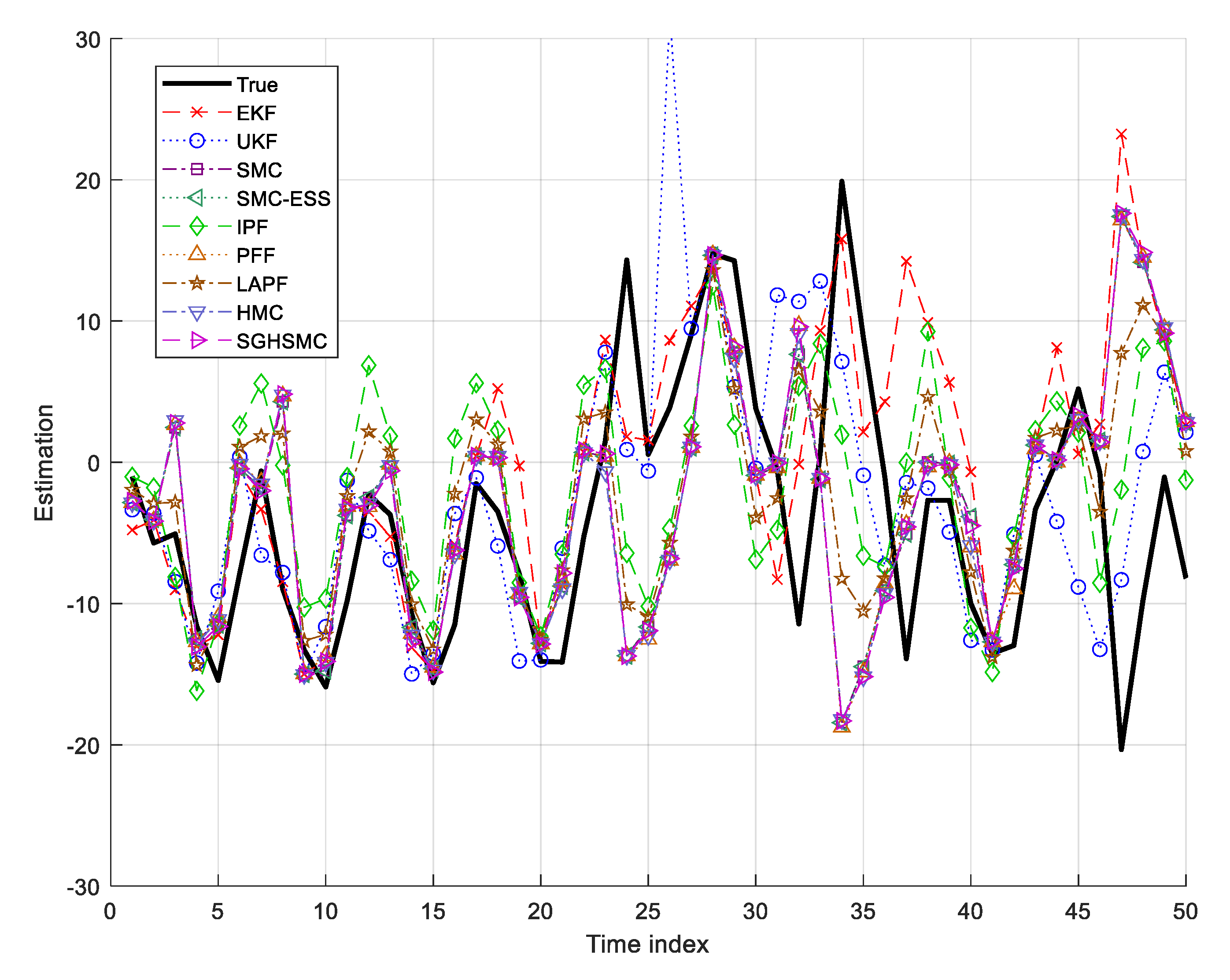
In Figure 1, we compare the tracking performance of all filters for the UNGM scenario, with both qualitative trajectories and quantitative metrics from

Table 1. RMSE of filters in simulation and experiment.

Type of Filter	Simulation (UNGM)	Experiment Case 1	Experiment Case 2
EKF	13.629	0.459	1.254
UKF	7.102	0.376	0.891
SMC	6.413	0.286	0.409
SMC-ESS	6.427	0.291	0.411
IPF	6.012	0.275	0.326
PFF	6.168	0.221	0.295
LAPF	6.0811	0.235	0.301
HMC	5.778	0.204	0.307
SGHSMC	5.068	0.106	0.286

Experiment unit: m.

and

Table 2. Computation time of filters in simulation and experiment.

Type of Filter	Simulation (UNGM)	Experiment Case 1	Experiment Case 2
EKF	0.14	1.46	0.80
UKF	1.11	3.09	2.11
SMC	1.33	148.87	134.87
SMC-ESS	1.20	147.11	133.29
IPF	2.26	326.40	321.05
PFF	6.56	537.67	640.92
LAPF	4.21	298.31	260.14
HMC	178.21	840.97	828.91
SGHSMC	4.74	295.22	254.74

Unit: msec.

. The UNGM’s strong nonlinearity and bimodal characteristics become particularly evident during time steps 10–15, 30–35, and 40–45. The EKF shows the largest performance degradation, with an RMSE of 13.629 m and a computation time of 0.14 ms per update, struggling particularly in these highly nonlinear regions due to its inherent linearization assumptions. The UKF performs better, with an RMSE of 7.102 m and a 1.11 ms computation time, but still fails to adequately capture the bimodal state distribution.

Among the particle-based methods, the standard SMC filter achieves an RMSE of 6.413 m, with a 1.33 ms computation time, showing improved tracking but an occasional loss of accuracy during rapid state transitions. The HMC variant demonstrates better performance, with an RMSE of 5.778 m, though at the cost of a significantly increased computational overhead (178.21 ms per update). In addition, the SMC-ESS filter achieves an RMSE of 6.427 m, slightly higher than that of the standard SMC filter (6.413 m), but with a marginally improved computational efficiency at 1.20 ms versus 1.33 ms. This suggests that the adaptive resampling strategy preserves computational resources without significant accuracy penalties in this highly nonlinear scenario. The LAPF demonstrates a more competitive performance, with an RMSE of 6.081 m in the UNGM simulation, positioning it between the standard SMC filter and advanced methods like the IPF. Its computation time of 4.21 ms represents a reasonable trade-off between performance and efficiency, falling significantly below that of the HMC framework (178.21 ms), while outperforming the standard SMC filter in accuracy.

The proposed SGHSMC filter demonstrates superior performance, achieving an RMSE of 5.068 m while maintaining an efficient computation time of 4.74 ms per update. This represents a 63% improvement in accuracy compared to the EKF and a 21% improvement compared to the standard SMC filter. The algorithm’s success in highly nonlinear regions can be attributed to its adaptive energy function and efficient state space exploration through stochastic gradient Hamiltonian dynamics. The IPF and PFF also show competitive performance (RMSEs of 6.012 m and 6.168 m, respectively) with varied computational requirements (2.26 ms and 6.56 ms, respectively, per update).

These quantitative results from Table 1 and Table 2 highlight the advantage of combining stochastic gradient information with Hamiltonian dynamics, particularly in scenarios where the state distribution exhibits strong nonlinearity and multimodality. The SGHSMC filter’s ability to maintain significantly lower RMSE values while keeping computational costs competitive demonstrates its effectiveness as a practical filtering solution.

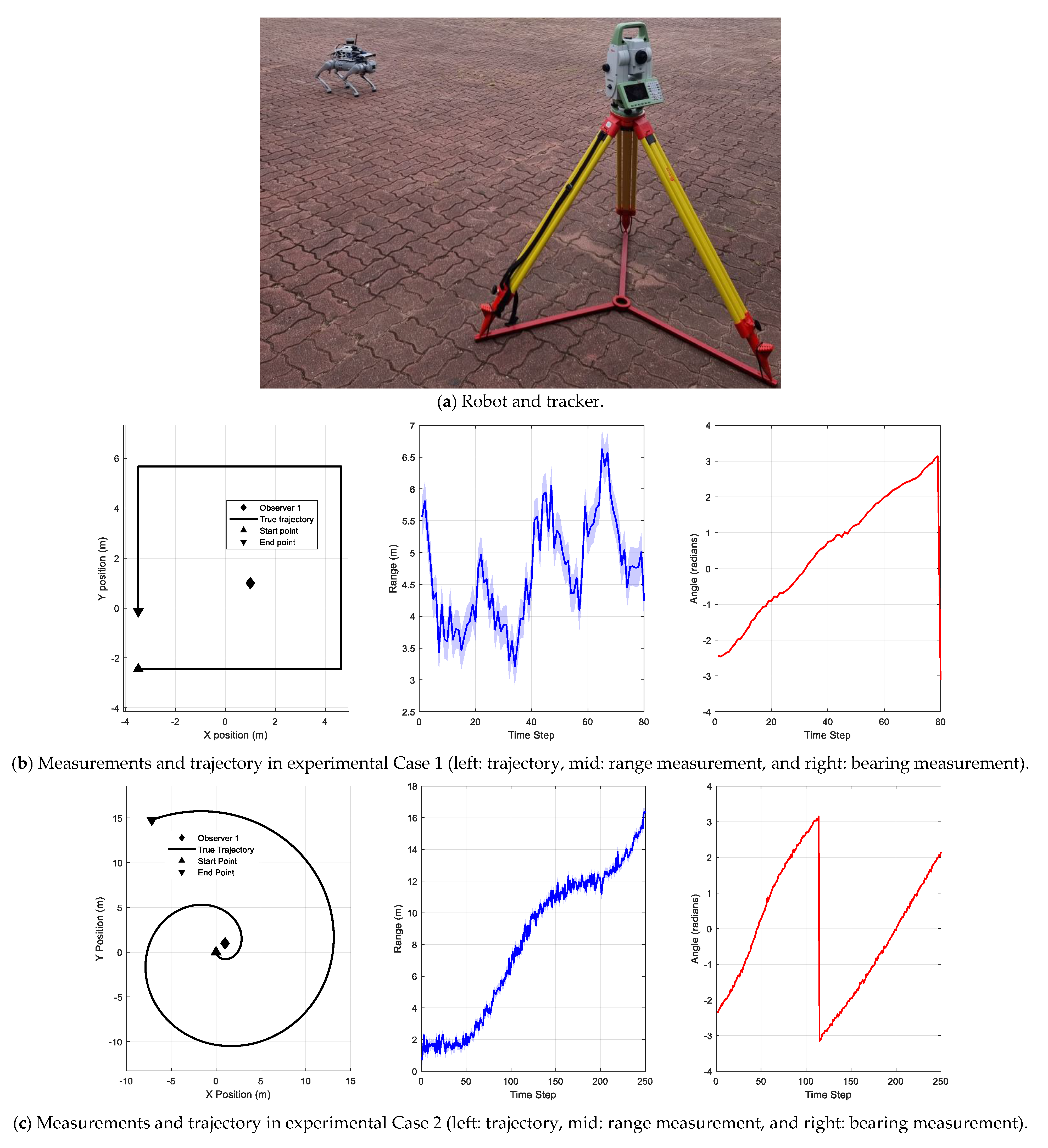
In the experiment, we applied the proposed algorithm to track a quadrupedal robot using a single Leica TS16 Total Station tracker (Figure 2), which provides both range and bearing measurements from a fixed observation point [22,23]. Figure 2 shows the experimental design and data. (a) The experimental setup showing the quadrupedal robot and Leica TS16 Total Station tracker positioned at a fixed observation point. (b) Rectangular trajectory experiment (Case 1) data visualization: the left panel shows the complete rectangular path with sharp 90 degree turns, creating a challenging tracking scenario; the middle panel displays the range measurements over time, showing characteristic plateaus during straight segments and rapid changes at corners; and the right panel shows the bearing measurements exhibiting distinct step-like patterns at each 90 degree turn. (c) Spiral trajectory experiment (Case 2) data visualization: the left panel shows the outward spiral path with a gradually increasing radius; the middle panel displays the range measurements that progressively increase as the target moves farther from the observation point, demonstrating the growing measurement uncertainty with distance; and the right panel shows the bearing measurements continuously changing as the target circles the observation point, creating a challenging scenario for angular tracking. The Leica TS16 Total Station tracker achieves an angle measurement precision of 3 arcseconds (equivalent to 1 milligon) and a range measurement accuracy of ±1 mm + 1.5 ppm. We assume a single moving target in the scene, with the tracking station positioned at a fixed location (1, 1) providing continuous range and bearing measurements. This setup creates a practical single-sensor tracking scenario where the measurement uncertainty increases with the target distance from the observation point, providing an excellent test case for evaluating the filter performance under varying measurement conditions. The state of the target at the time step $n$ consists of the position in two-dimensional cartesian coordinates, $x_{1,n}$ and $x_{2,n}$, and the velocity toward those coordinate axes, $x_{3,n}$ and $x_{4,n}$. Thus, the state vector can be expressed as follows:

$$x_n={\left(\begin{array}{cccc}{x}_{1,n}& x_{2,n}& x_{3,n}& x_{4,n}\end{array}\right)}^T$$

(16)

The dynamics of the target are modeled as a linear, discretized Wiener velocity model [7].

$$x_n=\left(\begin{array}{cccc}1& 0& \Delta t& 0\\ 0& 1& 0& \Delta t\\ 0& 0& 1& 0\\ 0& 0& 0& 1\end{array}\right)\left(\begin{array}{c}{x}_{1,n-1}\\ x_{2,n-1}\\ x_{3,n-1}\\ x_{4,n-1}\end{array}\right)+u_{n-1}$$

(17)

where $u_{n-1}$ is Gaussian noise with zero mean and covariance.

$$E\left[u_{n-1}{u}_{n-1}^T\right]=\left(\begin{array}{cccc}{\displaystyle \frac{1}{3}}\Delta t^3& 0& {\displaystyle \frac{1}{2}}\Delta t^2& 0\\ 0& {\displaystyle \frac{1}{3}}\Delta t^3& 0& {\displaystyle \frac{1}{2}}\Delta t^2\\ {\displaystyle \frac{1}{2}}\Delta t^2& 0& \Delta t& 0\\ 0& {\displaystyle \frac{1}{2}}\Delta t^2& 0& \Delta t\end{array}\right)u_s$$

(18)

where $u_s$ is the spectral density of the noise, which is set to $u_s=0.1$ in the experiment. The measurement model for the sensor $i$ is defined as follows:

$$y_n^i=\left[\begin{array}{c}\sqrt{{\left(x_{1,n}-s_1^i\right)}^2+{\left(x_{2,n}-s_2^i\right)}^2}\\ \arctan \left({\displaystyle \frac{x_{2,n}-s_2^i}{x_{1,n}-s_1^i}}\right)\end{array}\right]+v_n^i$$

(19)

This measurement model provides both range and bearing information from a single, stationary observation point, capturing the nonlinear relationship between the target state and measurements. In Equation (19), $\left(s_1^i,s_2^i\right)$ is the position of the sensor $i$ and $v_n^i~N\left(0,R\right)$, with $R=diag\left(\left[{0.3}^2\hspace{0.17em},\hspace{0.17em}{0.03}^2\right]\right)$. Moreover, 0.3 m is the standard deviation of the range measurement, and 0.03 radians is the standard deviation of the bearing measurement. In Figure 2b,c, we have plotted the measurements in radians obtained from both sensors. The sensor is placed to $\left(s_1^1,s_2^1\right)=\left(1,1\right)$.

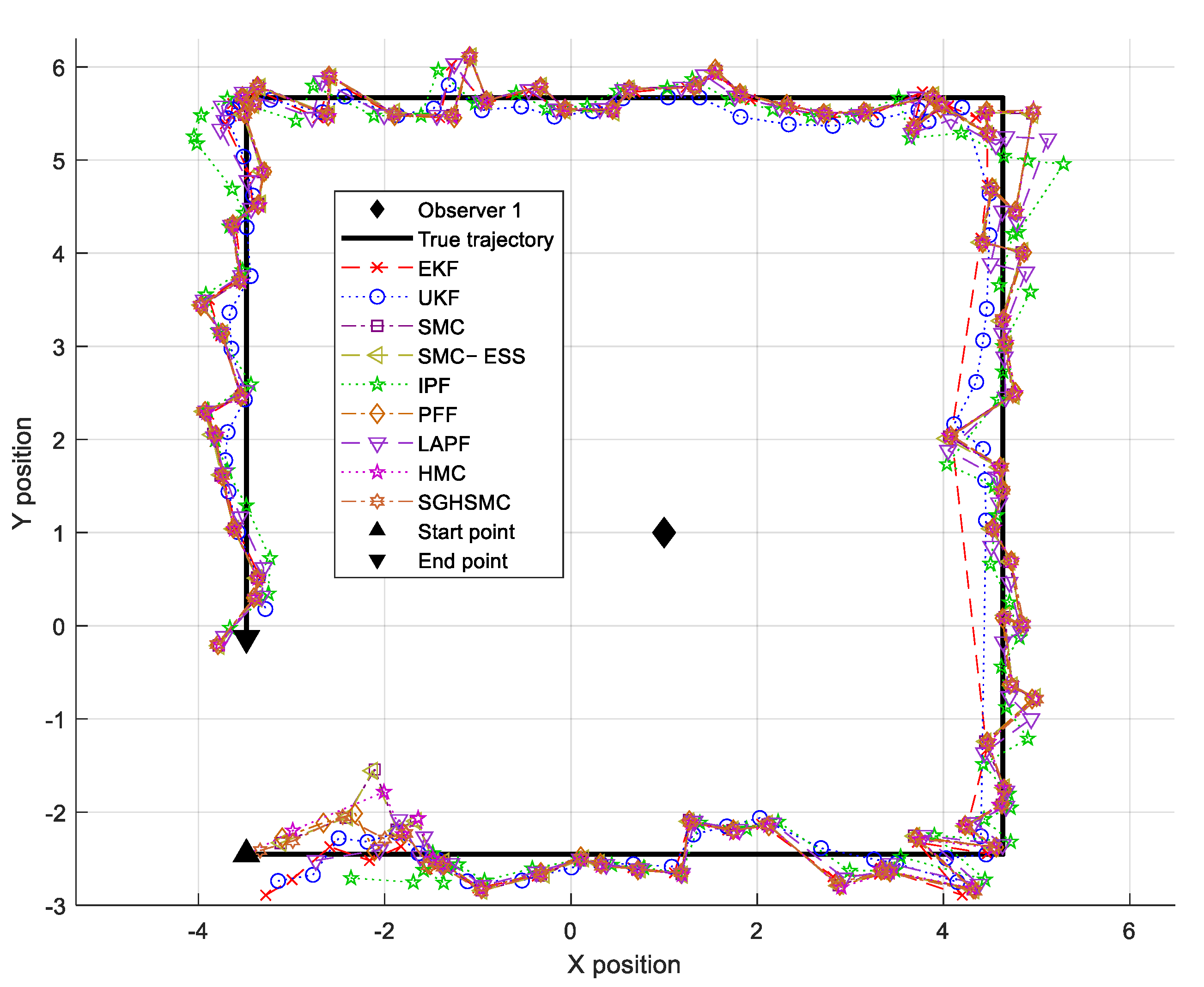
The experimental validation was conducted through two distinct scenarios, designed to evaluate the tracking performance under different motion patterns. For the rectangular trajectory (Experiment Case 1), we designed a path with four 90 degree turns at a constant speed, creating a 4 m × 4 m square pattern. For the spiral trajectory (Experiment Case 2), we implemented an outward spiral with a gradually increasing radius and velocity, specifically designed to test the filter performance under increasing range conditions.

Figure 3 presents the tracking results for the rectangular trajectory, where all filters face challenges during the sharp 90 degree turns. As shown in Table 1, the EKF achieves an RMSE of 0.459 m, while requiring a 1.46 ms computational time. The UKF shows improved accuracy, with an RMSE of 0.376 m, though at a higher computational cost of 3.09 ms. Traditional particle methods demonstrate better tracking capability, with the SMC filter achieving an RMSE of 0.286 m, albeit with a significant computational overhead (148.87 ms).

Notably, advanced particle methods show superior performance in this scenario. The HMC framework achieves an RMSE of 0.204 m, while our proposed SGHSMC filter demonstrates the best accuracy, with an RMSE of 0.106 m. The IPF and PFF also perform well, with RMSEs of 0.275 m and 0.221 m, respectively. However, these improved accuracies come with varying computational costs, as shown in Table 2. The SGHSMC filter maintains reasonable efficiency at 295.22 ms, while the HMC framework requires 840.97 ms per update.

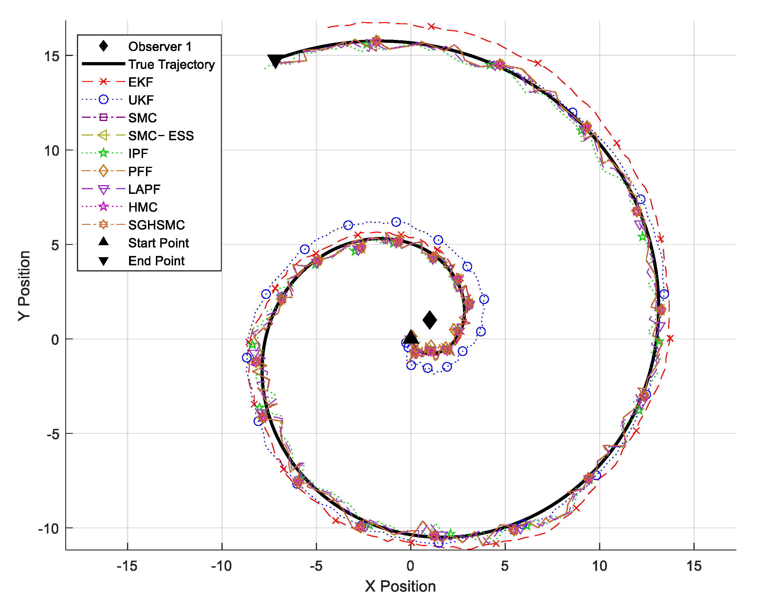
Figure 4 showcases the results from the spiral trajectory test, where increasing distance from the observation point presents additional challenges. In this scenario, the EKF’s RMSE increases to 1.254 m, and the UKF’s to 0.891 m, reflecting the growing difficulty of tracking greater distances. The SMC filter maintains better accuracy, with an RMSE of 0.409 m. The SGHSMC filter continues to demonstrate superior performance, with an RMSE of 0.286 m, while requiring a 254.74 ms computational time—notably more efficient than most other particle-based methods in this scenario.

The IPF and PFF also maintain good accuracy (0.326 m and 0.295 m RMSE, respectively), but require significantly more computational time (321.05 ms and 640.92 ms). The HMC framework achieves an RMSE of 0.307 m, but at the highest computational cost of 828.91 ms per update.

In the case of the adaptive filters, for the rectangular trajectory (Experiment Case 1), the SMC-ESS filter achieves an RMSE of 0.291 m, with a computation time of 147.11 ms, while the LAPF improves its accuracy to 0.235 m at a higher but still reasonable computational cost of 298.31 ms. Similarly, in the spiral trajectory (Experiment Case 2), the SMC-ESS filter and the LAPF achieve RMSEs of 0.411 m and 0.301 m, respectively, with the LAPF’s look-ahead strategy being particularly beneficial in predicting the continuous trajectory change. Notably, while both methods offer performance improvements over the standard SMC filter, neither matches the accuracy of the proposed SGHSMC approach, which maintains superior performance across all test scenarios. This highlights the advantages of combining stochastic gradient information with Hamiltonian dynamics in challenging nonlinear tracking applications.

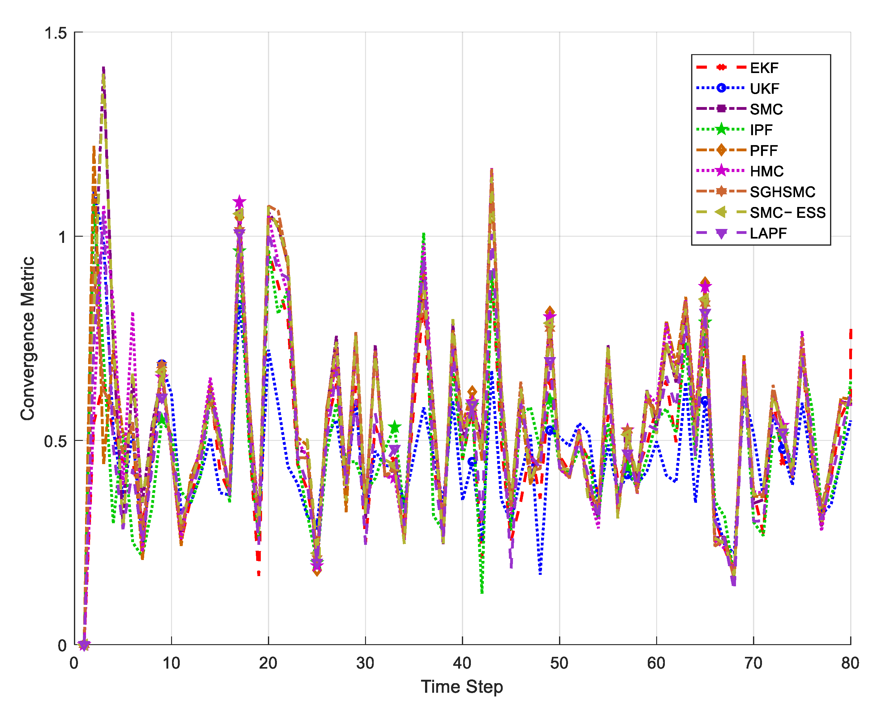
Additionally, to provide a more comprehensive analysis of the filter performance, we validated the stability of each filter through convergence metrics. While the convergence properties were theoretically analyzed in Section 2.3, it is essential to verify these trends with actual experimental data. To this end, Figure 5 and Figure 6 visualize the convergence metrics for each filter over time steps in the rectangular and spiral trajectories, respectively. This metric is calculated as the Euclidean distance between the consecutive state estimates, with lower values indicating more stable filter convergence.

Figure 5 illustrates the convergence metrics for each filter over time steps in the rectangular trajectory experiment. The convergence metric is measured as the Euclidean distance between the consecutive state estimates, representing the filter’s stability and consistency. Lower values indicate the more stable convergence of the filter. As shown in the graph, the EKF (red) exhibits the highest convergence metric, particularly at sharp directional changes, demonstrating its instability in nonlinear environments. While the UKF (blue) shows improvement over the EKF, it still struggles with abrupt changes. In contrast, the proposed SGHSMC (deep purple) filter maintains the lowest and most consistent convergence metric, showing stable convergence characteristics even at trajectory corners. This demonstrates how the adaptive energy function of the SGHSMC filter effectively responds to rapid state changes.

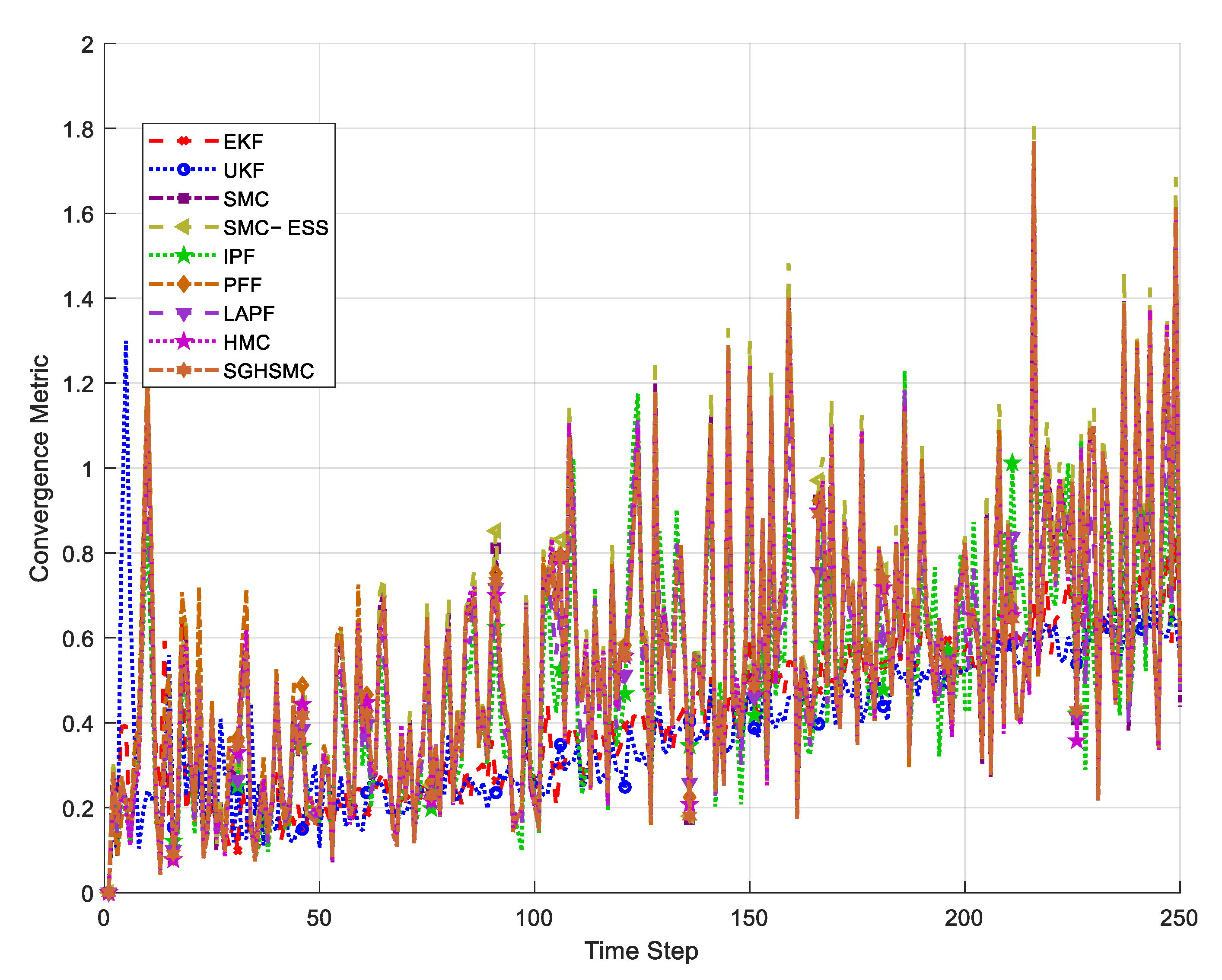
Figure 6 presents the convergence metric results for the spiral trajectory experiment. The spiral trajectory introduces additional challenges, with continuously changing curvature and increased uncertainty due to growing measurement distances. In this experiment, the SGHSMC filter maintains a remarkably stable convergence metric throughout the entire trajectory. Notably, while the EKF and UKF diverge sharply in the latter part of the trajectory, the SGHSMC filter maintains its stability. This demonstrates that the proposed method provides a robust performance even in complex situations with increasing measurement uncertainty. While the IPF and LAPF also show good convergence, the SGHSMC filter provides a more consistent performance, particularly in regions with rapid state changes.

These results highlight the SGHSMC filter’s consistently superior performance across both scenarios, achieving the lowest RMSE while maintaining better computational efficiency compared to other advanced particle methods. The improvement is particularly notable in the rectangular trajectory case, where the SGHSMC filter’s RMSE of 0.106 m represents a 77% improvement compared to the EKF and a 63% improvement compared to the standard SMC filter. A key implementation feature of the SGHSMC filter is its adaptive parameter adjustment mechanism. The friction coefficient ($\gamma$) and mass matrix ($M$) automatically adapt based on the state dynamics. These adaptive parameters significantly contribute to the SGHSMC filter’s superior performance, particularly evident in the spiral trajectory scenario (Figure 4), where the measurement uncertainty increases with distance. The computational overhead of these adaptations remains minimal, as shown in Table 2, where the SGHSMC filter maintains an average processing time of 4.74 ms in simulation despite the additional calculations, though experimental implementations require higher processing times of 295.22 ms and 254.74 ms for the two test cases.

4. Conclusions

This paper introduced the SGHSMC algorithm for nonlinear state estimation, featuring an adaptive energy function design that automatically adjusts to the target dynamics. Through extensive validation using both UNGM simulations and range-bearing tracking experiments, the SGHSMC filter demonstrated a superior performance compared to traditional and advanced filtering methods. In the UNGM scenario, it showed robust handling of strong nonlinearities and bimodal distributions, while in practical tracking experiments, it achieved significant improvements in accuracy (77% over the EKF in rectangular trajectories and 77.2% in spiral trajectories).

The experimental results highlight the key advantages of our approach: the effective handling of varying target dynamics through adaptive energy functions, efficient state estimation through stochastic gradient implementation, and robust performance under degrading measurement conditions. These results suggest that the SGHSMC filter provides a promising foundation for developing advanced tracking solutions that balance accuracy with computational efficiency.

Future work will focus on extending the framework to multi-target tracking scenarios and investigating applications in distributed sensor networks.