Optimizing Finite Population Mean Estimation Using Simulation and Empirical Data

Abstract

Two-phase sampling is an effective sampling approach that is useful in sample surveys when prior auxiliary information is not available. When two variables have an association, the ranks of the auxiliary variable are proportional to the study variable. Therefore, we can use these rankings to improve the accuracy of the estimators. In this article, we estimate the overall mean of the study variable based on extreme values and the ranks of the auxiliary variable. The properties of the proposed estimators with respect to biases and mean squared errors (MSEs) in two-phase sampling are obtained up to first order approximation. We verify the theoretical results and assess the performance of the proposed estimators using three datasets and a simulation study, which show that the proposed estimators outperform other existing estimators in terms of percent relative efficiency (PRE).

1. Introduction

Utilizing auxiliary data in survey sampling plays a significant role in enhancing the accuracy of estimators. To achieve better relative efficiency, methods such as ratio, regression, and product estimators incorporate supplementary details in addition to the primary study variables. For example, when estimating total household income, auxiliary metrics like the number of household members and overall expenditure can be helpful. Researchers have carried out extensive investigations to develop more effective estimators for various population parameters, including the mean, total, and median. Further insights into these improved estimators and their statistical characteristics can be found in related studies, see [1,2,3,4,5] and references therein.

In the field of sampling theory, the use of auxiliary variables alongside the primary variable of interest is a widely recognized strategy to enhance the efficiency and accuracy of survey designs. This approach takes advantage of the correlation between the auxiliary and main variables to yield more reliable estimations. In many practical situations, the population mean of the variable under study is not known prior to data collection. In such cases, researchers often rely on a dual-phase sampling approach, also known as double sampling. This strategy involves conducting an initial phase to gather basic information, followed by a second phase focused on more detailed data collection. Typically, a large preliminary sample is drawn to collect data on auxiliary variables, and a smaller, more focused sample is then selected either from the initial group or independently, to observe both the auxiliary and study variables. Due to its efficiency and lower cost, dual-phase sampling is a valuable tool in survey research, particularly when prior knowledge of auxiliary data is lacking. A brief review of two-phase sampling was first introduced in [6,7]. Recently, two-phase sampling has gained significant attention because of its cost-effectiveness in screening variables. Several studies have explored different aspects of two-phase sampling, including [8,9,10,11,12,13,14,15,16,17].

Survey data can sometimes include outliers or unusually large or small values, which may affect the reliability of statistical estimations. The presence of such extreme observations can distort the sample mean, potentially resulting in biased inferences. To address this, the authors in [18] initially introduced two estimators based on linear transformations involving the minimum and maximum values of known auxiliary variables. However, this approach did not receive much attention until it was later revisited in [19], who proposed improved ratio, product, and regression estimators by incorporating extreme value information of auxiliary variables for estimating population means. Building upon this, the authors in [20] extended these ideas within a dual-phase sampling framework to enhance estimation accuracy. The authors in [21] also explored different transformation techniques using extreme values of auxiliary variables to estimate the finite population mean. Further advancement was made by the authors in [22], who suggested innovative methods for estimating the mean under stratified random sampling designs that account for extreme values. Additionally, the authors in [23] introduced a novel group of estimators aimed at calculating population variance with minimal mean squared error by utilizing extreme value information. Most recently, the authors of [24,25,26] proposed several new classes of efficient estimators for population variance by applying transformation strategies to extreme values. For more details, see [27,28,29,30,31,32] and references therein.

Although the removal of extreme observations from survey data might appear beneficial, retaining them can offer valuable insights, especially when auxiliary variables are involved. Classical estimators often suffer from increased mean square error (MSE) in the presence of such values, leading to reduced efficiency. Rather than excluding these outliers, this study treats the minimum and maximum values of auxiliary variables as informative features. Inspired by the work of [22,23], we introduce two innovative families of estimators that incorporate these extremes values and ranks of auxiliary data to enhance the estimation of the finite population mean within a two-phase sampling framework.

• Real-life relevance of the proposed estimators

The proposed estimators are not only theoretically efficient but also highly applicable in practical settings where auxiliary information is partially available. In many real-world surveys, it is common to have access to auxiliary variables during a preliminary phase, while collecting detailed data on the study variable may be expensive or time-consuming. In such cases, utilizing the ranks and extreme values of auxiliary variables can significantly enhance the accuracy of population mean estimation. The following examples illustrate typical scenarios where the proposed methodology can be effectively applied:

• Agricultural Surveys: When estimating average crop yield in a region, data on the number of acres cultivated (auxiliary variable) may be available from administrative records. The ranks (e.g., top 10 largest farms) and extreme values (smallest and largest land holdings) can enhance estimation accuracy, especially in two-phase sampling where detailed crop yield data is expensive to collect.
• Public health studies: To estimate the average healthcare expenditure across households, auxiliary data like income levels or family size from census data can be used. Ranks of income groups (e.g., lowest and highest quintiles) and extreme income values can help refine estimates, particularly when full income data is unavailable in the first phase.
• Educational statistics: In assessing the average test scores of students across a district, school-level data such as the number of teachers or school enrollment (auxiliary variables) are readily available. Using the ranks of schools based on size or resources, along with the extremes (smallest and largest schools), can improve estimates with limited test score data in the second phase.
• Socioeconomic surveys: In household income and expenditure surveys, auxiliary variables like electricity usage or mobile phone ownership can be ranked, and extreme values (e.g., zero usage or very high usage) can serve as indicators to better estimate average household income.

The article is organized as follows: Section 2 outlines the methodology of the study and introduces the notation used throughout the paper. A review of the existing estimators is provided in Section 3. In Section 4, we present a detailed discussion of the newly proposed classes of estimators. Section 5 offers an in-depth mathematical comparison of these estimators. The simulation study, outlined in Section 6, generates six distinct artificial populations using various probability distributions, validating the theoretical results discussed in Section 5. This section also includes numerical examples that demonstrate the practical applications of the theoretical findings. Finally, Section 7 summarizes the main conclusions of the study and proposes directions for future research.

2. Methodology and Notation

Consider a finite population $U=\left(U_1,U_2,U_3,\dots ,U_N\right)$ consisting of N units. Let $y_i$ be the value of the study variable $Y,$ let $x_i$ denote the value of the auxiliary variable X, and let $w_i$ be the rank of the auxiliary variable W for the $ith$ unit.

Let the population data $X=\{x_1,x_2,\dots x_n,\dots ,x_m,\dots ,x_N\}.$ The sample data collected in the first phase is denoted by $X_1=\{x_1,x_2,\dots ,x_m\}$, while the second phase sample data is represented by $X_2=\{x_1,x_2,\dots ,x_n\}$. In this paper, we propose two improved classes of estimators to estimate the finite population mean $\overline{Y}$ of Y in the presence of auxiliary variable X. The definition of the two-phase sampling scheme is as follows:

1.

In the first phase, a simple random sample without replacement of size $\left(m<N\right)$ is drawn from the population to provide an estimate of the population mean $\overline{X}$, allowing for an initial approximation before further analysis.

2.

In the second phase, a simple random sample without replacement of n observations (where $n<m$) is selected to observe the variables y and x, allowing for more precise measurements and further analysis of the relationship between them.

Suppose the average values for the main study variable ($\overline{Y}$), the auxiliary variable ($\overline{X}$), and the corresponding ranks of the auxiliary variable ($\overline{W}$) are described as follows:

$$\overline{Y}={\displaystyle \frac{1}{N}}\sum _{i=1}^N{Y}_i,$$

(1)

$$\overline{X}={\displaystyle \frac{1}{N}}\sum _{i=1}^N{X}_i,$$

(2)

and

$$\overline{W}={\displaystyle \frac{1}{N}}\sum _{i=1}^N{W}_i.$$

(3)

The list of the important variables and different notations are given in

Table 1. List of important variable notations under a two-phase sampling design.

Symbol	Meaning	Symbol	Meaning
Y	Study variable	X	Auxiliary variable
W	Rank of auxiliary variable	$\overline{Y}$	Population mean of Y
$\overline{X}$	Population mean of X	$\overline{W}$	Population mean of W
$S_y^2$	Population variance of Y	$S_x^2$	Population variance of X
$S_w^2$	Population variance of W	$C_y$	Coefficient of variation of Y
$C_x$	Coefficient of variation of X	$C_w$	Coefficient of variation of W
${\rho }_{yx}$	Correlation between Y and X	${\rho }_{yw}$	Correlation between Y and W
${\rho }_{xw}$	Correlation between X and W	m	First-phase sample size
n	Second-phase sample size	N	Population size
${\theta }_1,{\theta }_2,{\theta }_3$	Sampling fractions	$Q_1$	Usual unbiased estimator
$Q_2,Q_3,\dots ,Q_6$	Existing estimators	$T,T_e$	Proposed estimators
$e_0,e_1,e_2,e_3,e_4$	Error terms

.

Define the population variances under simple random sampling without replacement (SRSWOR) for the study variable (Y), the auxiliary variable (X), and the ranked values of the auxiliary variable (W) as follows:

$$S_y^2={\displaystyle \frac{1}{N-1}}\sum _{i=1}^N{\left(Y_i-\overline{Y}\right)}^2,$$

(4)

$$S_x^2={\displaystyle \frac{1}{N-1}}\sum _{i=1}^N{\left(X_i-\overline{X}\right)}^2,$$

(5)

and

$$S_w^2={\displaystyle \frac{1}{N-1}}\sum _{i=1}^N{\left(W_i-\overline{W}\right)}^2,$$

(6)

respectively. Moreover, the population-level coefficients of variation corresponding to these variables are expressed as follows:

$$C_y={\displaystyle \frac{S_y}{\overline{Y}}},$$

(7)

$$C_x={\displaystyle \frac{S_x}{\overline{X}}},$$

(8)

and

$$C_w={\displaystyle \frac{S_w}{\overline{W}}},$$

(9)

respectively. We also know that the population correlation coefficients between Y and X, Y and W, as well as X and W are given by

$${\rho }_{yx}={\displaystyle \frac{S_{yx}}{S_y{S}_x}},$$

(10)

$${\rho }_{yw}={\displaystyle \frac{S_{yw}}{S_y{S}_w}},$$

(11)

and

$${\rho }_{xw}={\displaystyle \frac{S_{xw}}{S_x{S}_w}}.$$

(12)

Simple random sampling without replacement is used to estimate the unknown population mean $\overline{Y}$. In the first phase, a random sample of m units is selected from the population. The sample means ${\overline{x}}_1$ and ${\overline{w}}_1$ for the auxiliary variable X and its ranked version W are computed from this initial sample as follows:

$$\overline{x_1}={\displaystyle \frac{1}{m}}\sum _{i=1}^m{X}_i,$$

(13)

$$\overline{w_1}={\displaystyle \frac{1}{m}}\sum _{i=1}^m{W}_i,$$

(14)

while the first phase sample variances are expressed as

$$s_{x_1}^2={\displaystyle \frac{1}{m-1}}\sum _{i=1}^m{\left(X_i-{\overline{x}}_1\right)}^2,$$

(15)

and

$$s_{w_1}^2={\displaystyle \frac{1}{m-1}}\sum _{i=1}^m{\left(W_i-{\overline{w}}_1\right)}^2.$$

(16)

Additionally, let $\overline{y}$, ${\overline{x}}_2$, and ${\overline{w}}_2$ denote the sample means of the variables Y, X, and W, respectively, calculated from the second-phase sample of size n, such that

$$\overline{y}={\displaystyle \frac{1}{n}}\sum _{i=1}^n{Y}_i,$$

(17)

$$\overline{x_2}={\displaystyle \frac{1}{n}}\sum _{i=1}^n{X}_i,$$

(18)

and

$$\overline{w_2}={\displaystyle \frac{1}{n}}\sum _{i=1}^n{W}_i.$$

(19)

The second phase without replacement sample variances for these variables are defined as

$$s_y^2={\displaystyle \frac{1}{n-1}}\sum _{i=1}^n{\left(Y_i-\overline{y}\right)}^2,$$

(20)

$$s_{x_2}^2={\displaystyle \frac{1}{n-1}}\sum _{i=1}^n{\left(X_i-{\overline{x}}_2\right)}^2,$$

(21)

and

$$s_{w_2}^2={\displaystyle \frac{1}{n-1}}\sum _{i=1}^n{\left(W_i-{\overline{w}}_2\right)}^2.$$

(22)

3. Some Existing Estimators

In this section, we evaluate the bias and mean squared error characteristics of existing methods used to estimate the finite population mean and present a comparison with the newly proposed estimator classes.

The usual unbiased estimator to estimate the population mean $\overline{y}={\widehat{Q}}_1$ was proposed in [6], which is given by

$${\widehat{Q}}_1={\displaystyle \frac{1}{n}}\sum _{i=1}^n{y}_i.$$

(23)

The variance of ${\widehat{Q}}_1$ is given by

$$Var\left({\widehat{Q}}_1\right)={\theta }_2{Q}_1^2{C}_y^2,$$

(24)

where

$$\overline{Y}=Q_1,$$

represents the finite population mean in the two phase sampling method, and

$${\theta }_2=\left({\displaystyle \frac{N-n}{nN}}\right),$$

denotes a sampling fraction difference or correction term applied to account for variations in sample sizes during the second phase.

The authors in [7] suggested that a ratio type estimator for $Q_1$ in two-phase sampling be defined as

$${\widehat{Q}}_2={\widehat{Q}}_1\left({\displaystyle \frac{{\overline{x}}_2}{{\overline{x}}_1}}\right).$$

(25)

The expressions for bias and mean squared error (MSE) of ${\widehat{Q}}_2$ are expressed as follows:

$$Bias\left({\widehat{Q}}_2\right)\cong {\theta }_3{Q}_1\left(C_x^2-C_{yx}\right),$$

(26)

and

$$MSE\left({\widehat{Q}}_2\right)\cong Q_1^2\left({\theta }_1{C}_y^2+{\theta }_3{C}_x^2-2{\theta }_3{C}_{yx}\right),$$

(27)

where

$${\theta }_1=\left({\displaystyle \frac{N-m}{mN}}\right),{\theta }_3=\left({\displaystyle \frac{m-n}{mn}}\right),$$

represent the first phase and inter phase sampling correction terms, respectively.

The classical regression estimator ${\widehat{Q}}_4$ under two-phase sampling was proposed in [7], which is defined as

$${\widehat{Q}}_3={\widehat{Q}}_1+b_{yx}\left({\overline{x}}_2-{\overline{x}}_1\right),$$

(28)

where $b_{yx}$ is the sample regression coefficient.

The bias and mean squared error (MSE) of ${\widehat{Q}}_4$ are expressed as follows:

$$Bias\left({\widehat{Q}}_3\right)\cong -{\theta }_3{\beta }_{yx}\left({\displaystyle \frac{{\Delta }_{12}}{S_{yx}}}-{\displaystyle \frac{{\Delta }_{03}}{S_x^2}}\right),$$

(29)

$$MSE\left({\widehat{Q}}_3\right)\cong Q_1^2{C}_y^2\left({\theta }_2-{\theta }_3{\rho }_{yx}^2\right),$$

(30)

where

$${\beta }_{yx}={\displaystyle \frac{S_{yx}}{S_x^2}},$$

and

$${\Delta }_{qt}={\displaystyle \frac{{\sum }_{i=1}^N{\left(Y_i-\overline{Y}\right)}^r{\left(X_i-\overline{X}\right)}^t}{N-1}}.$$

The authors in [13] introduced exponential ratio and product-type estimators as alternative approaches for improved estimation, which are defined as follows:

$${\widehat{Q}}_4={\widehat{Q}}_{1}exp\left({\displaystyle \frac{{\overline{x}}_2-{\overline{x}}_1}{{\overline{x}}_1+{\overline{x}}_2}}\right),$$

(31)

and

$${\widehat{Q}}_5={\widehat{Q}}_{1}exp\left({\displaystyle \frac{{\overline{x}}_1-{\overline{x}}_2}{{\overline{x}}_1+{\overline{x}}_2}}\right).$$

(32)

The expressions for mean squared error of ${\widehat{Q}}_5$ and ${\widehat{Q}}_6$ are defined as follows:

$$MSE\left({\widehat{Q}}_4\right)\cong Q_1^2\left[{\theta }_2{C}_y^2+{\theta }_3{C}_x^2\left({\displaystyle \frac{1}{4}}-\delta \right)\right],$$

(33)

and

$$MSE\left({\widehat{Q}}_5\right)\cong Q_1^2\left[{\theta }_2{C}_y^2+{\theta }_3{C}_x^2\left({\displaystyle \frac{1}{4}}+\delta \right)\right],$$

(34)

where

$$\delta =\left({\displaystyle \frac{{\rho }_{yx}}{C_x}}\right)C_y.$$

The authors in [14] proposed that a double sampling estimator for $Q_1$ is defined as

$${\widehat{Q}}_6\cong {\widehat{Q}}_1\left\{t\left({\displaystyle \frac{{\overline{x}}_2}{{\overline{x}}_1}}\right)+(1-t)\left({\displaystyle \frac{{\overline{x}}_1}{{\overline{x}}_2}}\right)\right\},$$

(35)

where

$$t={\displaystyle \frac{1+\delta }{2}}.$$

The expressions for bias and mean squared error (MSE) are expressed as follows:

$$Bias{\left({\widehat{Q}}_6\right)}_{min}\cong {\displaystyle \frac{1}{2}}{\theta }_3{Q}_1{C}_x^2\left[1+\delta \left(1-2\delta \right)\right],$$

(36)

and

$$MSE{\left({\widehat{Q}}_6\right)}_{min}\cong Q_1^2{C}_y^2\left[{\theta }_2(1-{\rho }_{yx}^2)+{\theta }_1{\rho }_{yx}^2\right].$$

(37)

4. Suggested an Improved Family of Estimators

In this section, we present enhanced estimators for estimating the finite population mean, based on the principles outlined in [22,23]. These estimators utilize the known extreme values of auxiliary variables, along with their ranks, within a two-phase sampling method to enhance the reliability of the results. The mathematical expressions for these estimators are outlined below:

$$\widehat{T}=\left[k_1{\widehat{Q}}_1{\left({\displaystyle \frac{{\overline{x}}_2}{{\overline{x}}_1}}\right)}^{t_1}+k_2{\left({\displaystyle \frac{{\overline{x}}_2}{{\overline{x}}_1}}\right)}^{t_2}\right]exp\left[{\displaystyle \frac{t_3\left({\overline{x}}_2-{\overline{x}}_1\right)}{t_3\left({\overline{x}}_1+{\overline{x}}_2\right)+2t_4}}\right]$$

(38)

and

$${\widehat{T}}_e={\widehat{Q}}_{1}exp\left[k_3\left.\left\{{\displaystyle \frac{\left({\overline{x}}_2-{\overline{x}}_1\right)}{\left({\overline{x}}_2-{\overline{x}}_1\right)+2t_5}}\right\}\right]\right.exp\left[k_4\left\{{\displaystyle \frac{\left({\overline{w}}_2-{\overline{w}}_1\right)}{\left({\overline{w}}_1+{\overline{w}}_2\right)+2t_6}}\right\}\right],$$

(39)

where the scalar parameters $(t_1,t_2)$ are restricted to the values $(0,-1,1)$, while $(k_1,k_2)$ represent unknown constants that require suitable selection to achieve reduced bias and lower mean squared error. On the other hand, $(k_3=k_4=2)$ are fixed known constants. The auxiliary variable parameters are represented by $t_3$ and $t_4$, whereas $t_5=X_M-X_m$ and $t_6=W_M-W_m$ indicate the range of values based on the maximum and minimum observations of the auxiliary variables. Additionally, various sub-forms of the proposed estimator-I are derived from Equation (38) and summarized in

Table 2. Various forms of estimator-I under a two-phase sampling design.

Subsets of $\widehat{\mathit{T}}$	${\mathit{t}}_1$	${\mathit{t}}_2$	${\mathit{t}}_3$	${\mathit{t}}_4$
${\widehat{T}}_1=\left[k_1{\widehat{Q}}_1\left({\displaystyle \frac{{\overline{x}}_2}{{\overline{x}}_1}}\right)+k_2\left({\displaystyle \frac{{\overline{x}}_1}{{\overline{x}}_2}}\right)\right]S$	1	−1	1	$(X_M-X_m)/\overline{X}$
${\widehat{T}}_2=\left[k_1{\widehat{Q}}_1\left({\displaystyle \frac{{\overline{x}}_1}{{\overline{x}}_2}}\right)+k_2\left({\displaystyle \frac{{\overline{x}}_2}{{\overline{x}}_1}}\right)\right]S$	−1	1	${\rho }_{yx}$	$(X_M-X_m)/\overline{X}$
${\widehat{T}}_3=\left[k_1{\widehat{Q}}_1\left({\displaystyle \frac{{\overline{x}}_1}{{\overline{x}}_2}}\right)+k_2\left({\displaystyle \frac{{\overline{x}}_1}{{\overline{x}}_2}}\right)\right]S$	−1	−1	$(X_M-X_m)/\overline{X}$	${\rho }_{yx}$
${\widehat{T}}_4=\left[k_1{\widehat{Q}}_4+k_2\left({\displaystyle \frac{{\overline{x}}_2}{{\overline{x}}_1}}\right)\right]S$	0	1	$(X_M-X_m)/\overline{X}$	${\beta }_{2\left(x\right)}$
${\widehat{T}}_5=\left[k_1{\widehat{Q}}_1\left({\displaystyle \frac{{\overline{x}}_2}{{\overline{x}}_1}}\right)+k_2\left({\displaystyle \frac{{\overline{x}}_2}{{\overline{x}}_1}}\right)\right]S$	1	1	$(X_M-X_m)/\overline{X}$	1
${\widehat{T}}_6=\left[k_1{\widehat{Q}}_1+k_2\left({\displaystyle \frac{{\overline{x}}_1}{{\overline{x}}_2}}\right)\right]S$	0	−1	${\beta }_{2\left(x\right)}$	$(X_M-X_m)/\overline{X}$
${\widehat{T}}_7=\left[k_1{\widehat{Q}}_1\left({\displaystyle \frac{{\overline{x}}_2}{{\overline{x}}_1}}\right)+k_2\right]S$	1	0	$(X_M-X_m)/\overline{X}$	$C_x$
${\widehat{T}}_8=\left[k_1{\widehat{Q}}_1\left({\displaystyle \frac{{\overline{x}}_1}{{\overline{x}}_2}}\right)+k_2\right]S$	−1	0	$C_x$	$(X_M-X_m)/\overline{X}$

.

where

$$S=exp\left[{\displaystyle \frac{t_3\left({\overline{x}}_2-{\overline{x}}_1\right)}{t_3\left({\overline{x}}_1+{\overline{x}}_2\right)+2t_4}}\right],$$

and

$${\displaystyle \frac{X_M-X_m}{\overline{X}}},$$

represents the normalized range of the auxiliary variable.

4.1. Properties of the Suggested Estimator-I

To analyze the properties of the first proposed class of estimators, we introduce the following error terms. Let

$$e_0=\left({\displaystyle \frac{{\widehat{Q}}_1-Q_1}{Q_1}}\right),e_1=\left({\displaystyle \frac{{\overline{x}}_1-\overline{X}}{\overline{X}}}\right),e_2=\left({\displaystyle \frac{{\overline{x}}_2-\overline{X}}{\overline{X}}}\right),e_3=\left({\displaystyle \frac{{\overline{w}}_1-\overline{W}}{\overline{W}}}\right),e_4=\left({\displaystyle \frac{{\overline{w}}_2-\overline{W}}{\overline{W}}}\right),$$

such that $E\left(e_i\right)=0$, $(i=0,1,2,3,4)$.

Additionally, $E\left(e_0^2\right)={\theta }_2{C}_y^2$, $E\left(e_1^2\right)={\theta }_2{C}_x^2$, $E\left(e_2^2\right)={\theta }_1{C}_x^2$, $E\left(e_3^2\right)={\theta }_2{C}_w^2$, $E\left(e_4^2\right)={\theta }_1{C}_w^2$, $E\left(e_0{e}_1\right)={\theta }_2{C}_{yx}$, $E\left(e_0{e}_2\right)={\theta }_1{C}_{yx}$, $E\left(e_0{e}_3\right)={\theta }_2{C}_{yw}$, $E\left(e_0{e}_4\right)={\theta }_1{C}_{yw}$, $E\left(e_1{e}_2\right)={\theta }_1{C}_x^2$, $E\left(e_1{e}_3\right)={\theta }_2{C}_{xw}$, $E\left(e_1{e}_4\right)={\theta }_1{C}_{xw}$, $E\left(e_2{e}_3\right)={\theta }_1{C}_{xw}$, $E\left(e_2{e}_4\right)={\theta }_1{C}_{xw}$, and $E\left(e_3{e}_4\right)={\theta }_2{C}_w^2.$

To explore the characteristics of the first proposed estimator, we express Equation (38) in terms of error components.

$$\begin{array}{c}\widehat{T}=\left[k_1{Q}_1\left(1+e_0\right){\left(1+e_1\right)}^{-t_1}{\left(1+e_2\right)}^{t_1}+k_2{\left(1+e_1\right)}^{-t_2}{\left(1+e_2\right)}^{t_2}\right]\times \hfill \\ exp\left[{\displaystyle \frac{v_1\left(e_2-e_1\right)}{2}}{\left(1+{\displaystyle \frac{v_1}{2}}\left(e_2+e_1\right)\right)}^{-1}\right],\hfill \end{array}$$

where

$$v_1={\displaystyle \frac{t_3\overline{X}}{t_3\overline{X}+t_4}}.$$

By applying a first-order Taylor series expansion, we derive

$$\begin{array}{c}\widehat{T}-Q_1\cong -Q_1+k_1{Q}_1\left[1+e_0-e_1\left(t_1+{\displaystyle \frac{v_1}{2}}\right)+e_2\left(t_1+{\displaystyle \frac{v_1}{2}}\right)+e_1^2\left({\displaystyle \frac{t_1{v}_1}{2}}+{\displaystyle \frac{3v_1^2}{8}}+{\displaystyle \frac{t_1\left(t_1+1\right)}{2}}\right)\right.\hfill \\ \left.+e_2^2\left({\displaystyle \frac{t_1{v}_1}{2}}-{\displaystyle \frac{v_1^2}{8}}+{\displaystyle \frac{t_1\left(t_1-1\right)}{2}}\right)-e_0{e}_1\left(t_1+{\displaystyle \frac{v_1}{2}}\right)-e_0{e}_2\left(t_1+{\displaystyle \frac{v_1}{2}}\right)-e_1{e}_2{\left(t_1+{\displaystyle \frac{v_1}{2}}\right)}^2\right]\hfill \\ +k_2\left[1-e_1\left(t_2+{\displaystyle \frac{v_1}{2}}\right)+e_2\left(t_2+{\displaystyle \frac{v_1}{2}}\right)+e_1^2\left({\displaystyle \frac{t_2{v}_1}{2}}+{\displaystyle \frac{3v_1^2}{8}}+{\displaystyle \frac{t_2\left(t_2+1\right)}{2}}\right)\right.\hfill \\ \left.+e_2^2\left({\displaystyle \frac{t_2{v}_1}{2}}-{\displaystyle \frac{v_1^2}{8}}+{\displaystyle \frac{t_2\left(t_2-1\right)}{2}}\right)\left.-e_1{e}_2{\left(t_2+{\displaystyle \frac{v_1}{2}}\right)}^2\right]\right].\hfill \end{array}$$

(40)

Using (40), the bias of $\widehat{T}$ is given by

$$Bias\left(\widehat{T}\right)\cong \left[-Q_1+k_1{Q}_1{A}_3+k_2{A}_5\right],$$

(41)

where

$$\begin{array}{c}{A}_3=\left[1+{\theta }_2\left\{C_x^2\left({\displaystyle \frac{4t_1\left(t_1+1+v_1\right)+3v_1^2}{8}}\right)-\left.C_{yx}\left({\displaystyle \frac{2t_1+v_1}{2}}\right)\right\}\right.\right.\hfill \\ +{\theta }_1\left\{C_x^2\left\{{\displaystyle \frac{-4t_1\left(t_1+v_1+1\right)-3v_1^2}{2}}\right\}\right.+\left.\left.C_{yx}\left({\displaystyle \frac{2t_1+v_1}{2}}\right)\right\}\right],\hfill \end{array}$$

and

$$A_5=\left[1+{\theta }_2{C}_x^2\left({\displaystyle \frac{4t_2\left(t_2+v_1+1\right)+3v_1^2}{8}}\right)+{\theta }_1{C}_x^2\left({\displaystyle \frac{-2t_2\left(t_2+v_1-1\right)-3v_1^2}{4}}\right)\right].$$

Squaring both sides of Equation (40) and then taking the expected value leads to the first-order mean squared error (MSE), which is expressed as follows:

$$MSE\left(\widehat{T}\right)\cong \left[Q_1^2+k_1^2{Q}_1^2{A}_1+k_2^2{A}_2-2k_1{Q}_1^2{A}_3-2k_2{Q}_1{A}_5+2k_1{k}_2{Q}_1{A}_4\right],$$

(42)

where

$$\begin{array}{c}{A}_1=\left[1+{\theta }_2\left\{C_y^2+C_x^2\left\{{\left(t_1+{\displaystyle \frac{v_1}{2}}\right)}^2+\left.\left(t_1{v}_1+{\displaystyle \frac{3v_1^2}{4}}+{\displaystyle \frac{t_1\left(t_1+1\right)}{2}}\right)\right\}\right.\right.\right.-\left.4C_{yx}\left(t_1+{\displaystyle \frac{v_1}{2}}\right)\right\}\hfill \\ +{\theta }_1\left\{C_x^2\left\{{\left(t_1+{\displaystyle \frac{v_1}{2}}\right)}^2\right.\right.+\left(t_1{v}_1-{\displaystyle \frac{v_1^2}{4}}+t_1\left(t_1-1\right)\right)\left.-4\left(t_1+{\displaystyle \frac{v_1}{2}}\right)\right\}+\left.\left.4C_{yx}\left(t_1+{\displaystyle \frac{v_1}{2}}\right)\right\}\right],\hfill \end{array}$$

$$\begin{array}{c}{A}_2=\left[1+{\theta }_2{C}_x^2\left\{{\left(t_2+{\displaystyle \frac{v_1}{2}}\right)}^2+\left.\left(t_2{v}_1+{\displaystyle \frac{3v_1^2}{4}}+t_2\left(t_2+1\right)\right)\right\}\right.\right.+{\theta }_1{C}_x^2\left\{{\left(t_2+{\displaystyle \frac{v_1}{2}}\right)}^2\right.\hfill \\ \left.\left.+\left(t_2{v}_1-{\displaystyle \frac{v_1^2}{4}}+t_2\left(t_2-1\right)\right)-4{\left(t_2+{\displaystyle \frac{v_1}{2}}\right)}^2\right\}\right],\hfill \end{array}$$

and

$$\begin{array}{c}{A}_4=\left[1+{\theta }_2\left\{C_x^2\left\{\left({\displaystyle \frac{t_1{v}_1}{2}}+{\displaystyle \frac{3v_1^2}{8}}+{\displaystyle \frac{t_1\left(t_1+1\right)}{2}}\right)+\left(t_1+{\displaystyle \frac{v_1}{2}}\right)\left(t_2+{\displaystyle \frac{v_1}{2}}\right)+\left({\displaystyle \frac{t_2{v}_1}{2}}+{\displaystyle \frac{3v_1^2}{8}}+{\displaystyle \frac{t_2\left(t_2+1\right)}{2}}\right)\right.\right.\right.\hfill \\ -\left.C_{yx}\left(t_1+t_2+v_1\right)\right\}+{\theta }_1\left\{C_x^2\left\{\left({\displaystyle \frac{t_1{v}_1}{2}}-{\displaystyle \frac{v_1^2}{8}}+{\displaystyle \frac{t_1\left(t_1-1\right)}{2}}\right)-\left(t_1+{\displaystyle \frac{v_1}{2}}\right)\left(t_2+{\displaystyle \frac{v_1}{2}}\right)\right.\right.\hfill \\ +\left({\displaystyle \frac{t_2{v}_1}{2}}-{\displaystyle \frac{v_1^2}{8}}+{\displaystyle \frac{t_2\left(t_2-1\right)}{2}}\right)\left.-{\left(t_1+{\displaystyle \frac{v_1}{2}}\right)}^2-{\left(t_2+{\displaystyle \frac{v_1}{2}}\right)}^2\right\}+C_{yx}(t_1+t_2+v_1)\left\}\right].\hfill \end{array}$$

To find the optimal values of $k_1$ and $k_2$, we minimize Equation (42), resulting in the following expressions:

$$k_{1\left(opt\right)}={\displaystyle \frac{A_2{A}_3-A_4{A}_5}{A_1{A}_2-A_4^2}},$$

and

$$k_{2\left(opt\right)}={\displaystyle \frac{Q_1\left(A_1{A}_5-A_3{A}_4\right)}{A_1{A}_2-A_4^2}}.$$

The bias and mean squared error (MSE) for $\widehat{T}$ are minimized by substituting the optimal values of $k_1$ and $k_2$ into Equations (41) and (42), leading to the following results:

$$Bias{\left(\widehat{T}\right)}_{min}\cong -Q_1^2\left[1-{\displaystyle \frac{\left(A_1{A}_5^2+A_2{A}_3^2-2A_3{A}_4{A}_5\right)}{A_1{A}_2-A_4^2}}\right],$$

(43)

and

$$MSE{\left(\widehat{T}\right)}_{min}\cong Q_1^2\left[1-{\displaystyle \frac{\left(A_1{A}_5^2+A_2{A}_3^2-2A_3{A}_4{A}_5\right)}{A_1{A}_2-A_4^2}}\right].$$

(44)

4.2. Properties of the Suggested Estimator-II

Next, we express Equation (39) in terms of error components to derive the bias and mean squared error (MSE) of the second proposed estimator ${\widehat{T}}_e,$ i.e.,

$$\begin{array}{c}{\widehat{T}}_e=Q_1\left(1+e_0\right)exp\left[k_3\left\{{\displaystyle \frac{v_2\left(e_2-e_1\right)}{2}}{\left(1+{\displaystyle \frac{v_2}{2}}\left(e_1+e_2\right)\right)}^{-1}\right\}\right]exp\left[k_4\left\{{\displaystyle \frac{v_3\left(e_4-e_3\right)}{2}}\right.\right.\hfill \\ \left.\left.{\left(1+{\displaystyle \frac{v_3}{2}}\left(e_3+e_4\right)\right)}^{-1}\right\}\right],\hfill \end{array}$$

(45)

where

$$t_2={\displaystyle \frac{\overline{X}}{\overline{X}+t_5}},$$

and

$$v_3={\displaystyle \frac{\overline{W}}{\overline{W}+t_6}}.$$

By applying a first-order Taylor expansion, we derive

$$\begin{array}{c}{\widehat{T}}_e-Q_1\cong Q_1\left[e_0-{\displaystyle \frac{k_3{v}_2}{2}}\left(e_1-e_2\right)-{\displaystyle \frac{k_4{v}_3}{2}}\left(e_3-e_4\right)+\left({\displaystyle \frac{k_3{v}_2^2}{4}}+{\displaystyle \frac{k_3^2{v}_2^2}{8}}\right)e_1^2-\left({\displaystyle \frac{k_3{v}_2^2}{4}}-{\displaystyle \frac{k_3^2{v}_2^2}{8}}\right)e_2^2\right.\hfill \\ +\left({\displaystyle \frac{k_4{v}_3^2}{4}}-{\displaystyle \frac{k_4^2{v}_3^2}{8}}\right)e_3^2-\left({\displaystyle \frac{k_4{v}_3^2}{4}}-{\displaystyle \frac{k_4^2{v}_3^2}{8}}\right)e_4^2-{\displaystyle \frac{k_3{v}_2}{2}}{e}_0{e}_1+{\displaystyle \frac{k_3{v}_2}{2}}{e}_0{e}_2-{\displaystyle \frac{k_4{v}_3}{2}}{e}_0{e}_3\hfill \\ +{\displaystyle \frac{k_4{v}_3}{2}}{e}_0{e}_4-{\displaystyle \frac{k_3^2{v}_2^2}{2}}{e}_1{e}_2+{\displaystyle \frac{k_3{k}_4{v}_2{v}_3}{4}}{e}_1{e}_3-{\displaystyle \frac{k_3{k}_4{v}_2{v}_3}{4}}{e}_1{e}_4-{\displaystyle \frac{k_3{k}_4{v}_2{v}_3}{4}}{e}_2{e}_3\hfill \\ \left.+{\displaystyle \frac{k_3{k}_4{v}_2{v}_3}{4}}{e}_2{e}_4-{\displaystyle \frac{k_4^2{v}_3^2}{2}}{e}_3{e}_4\right].\hfill \end{array}$$

(46)

Using (46), the bias of ${\widehat{T}}_e$ is given by

$$\begin{array}{c}Bias\left({\widehat{T}}_e\right)\cong {\theta }_2{Q}_1\left[\left({\displaystyle \frac{k_3^2{v}_2^2}{8}}+{\displaystyle \frac{k_3{v}_2^2}{4}}\right)C_x^2+\left({\displaystyle \frac{k_4^2{v}_3^2}{8}}+{\displaystyle \frac{k_4{v}_3^2}{4}}\right)C_w^2-{\displaystyle \frac{k_3{v}_2}{2}}{C}_{yx}\right.-{\displaystyle \frac{k_4{v}_3}{2}}{C}_{yw}\hfill \\ \left.+{\displaystyle \frac{k_3{k}_4{v}_2{v}_3}{2}}{C}_{xw}\right]-{\theta }_1{Q}_1\left[\left({\displaystyle \frac{k_3^2{v}_2^2}{8}}+{\displaystyle \frac{k_3{v}_2^2}{4}}\right)C_x^2+\left({\displaystyle \frac{k_4^2{v}_3^2}{8}}+{\displaystyle \frac{k_4{v}_3^2}{4}}\right)C_w^2\right.\hfill \\ -{\displaystyle \frac{k_3{v}_2}{2}}{C}_{yx}-{\displaystyle \frac{k_4{v}_3}{2}}{C}_{yw}+\left.{\displaystyle \frac{k_3{k}_4{v}_2{v}_3}{2}}{C}_{xw}\right].\hfill \end{array}$$

(47)

After squaring both sides of (46) and applying the expected value, we obtain a first-order mean squared error (MSE) as shown below:

$$\begin{array}{c}MSE\left({\widehat{T}}_e\right)\cong {\theta }_2{Q}_1^2\left[C_y^2+{\displaystyle \frac{k_3^2{v}_2^2}{4}}{C}_x^2+{\displaystyle \frac{k_4^2{v}_3^2}{4}}{C}_w^2-k_3{v}_2{C}_{yx}-k_4{v}_3{C}_{yw}\right.\left.+{\displaystyle \frac{k_3{k}_4{v}_2{v}_3}{2}}{C}_{xw}\right]\hfill \\ -{\theta }_1{Q}_1^2\left[{\displaystyle \frac{k_3^2{v}_2^2}{4}}{C}_x^2+{\displaystyle \frac{k_4^2{v}_3^2}{4}}{C}_w^2-k_3{v}_2{C}_{yx}-k_4{v}_3{C}_{yw}+{\displaystyle \frac{k_3{k}_4{v}_2{v}_3}{2}}{C}_{xw}\right].\hfill \end{array}$$

(48)

After substituting the known values for $k_3$ and $k_4$ into Equations (47) and (48), we can express the bias and MSE for ${\widehat{T}}_e$. With a few simplifications, the resulting expressions are as follows:

$$Bias\left({\widehat{T}}_e\right)\cong {\theta }_3{Q}_1\left[{\displaystyle \frac{3}{2}}\left(v_2^2{C}_x^2+v_3^2{C}_w^2\right)-\left(v_2{C}_{yx}+v_3{C}_{yw}-{\displaystyle \frac{1}{2}}{v}_2{v}_3{C}_{xw}\right)\right],$$

(49)

and

$$MSE\left({\widehat{T}}_e\right)\cong Q_1^2\left[{\theta }_2{C}_y^2+{\theta }_3\left(v_2^2{C}_x^2+v_3^2{C}_w^2-2v_2{C}_{yx}-2v_3{C}_{yw}+2v_2{v}_3{C}_{xw}\right)\right].$$

(50)

5. Mathematical Comparison

In this section, the suggested estimators $\widehat{T}$ and ${\widehat{T}}_e$ are compared with existing estimators, including ${\widehat{Q}}_1$, ${\widehat{Q}}_2$, ${\widehat{Q}}_3$, ${\widehat{Q}}_4$, ${\widehat{Q}}_5,$ and ${\widehat{Q}}_6$.

5.1. Suggested Estimator-I

Condition (i): By (24) and (44),

$$\begin{gathered} Var\left({\widehat{Q}}_1\right)>MSE{\left(\widehat{T}\right)}_{min}\mathrm{if} \\ {\theta }_2{C}_y^2+\left({\displaystyle \frac{A_1{A}_5^2+A_2{A}_3^2-2A_3{A}_4{A}_5}{A_1{A}_2-A_4^2}}\right)>1. \end{gathered}$$

Condition (ii): By (27) and (44),

$$\begin{gathered} MSE\left({\widehat{Q}}_2\right)>MSE{\left(\widehat{T}\right)}_{min}\mathrm{if} \\ \left({\theta }_2{C}_y^2+{\theta }_3{C}_x^2-2{\theta }_3{C}_{yx}\right)+\left({\displaystyle \frac{A_1{A}_5^2+A_2{A}_3^2-2A_3{A}_4{A}_5}{A_1{A}_2-A_4^2}}\right)>1. \end{gathered}$$

Condition (iii): By (30) and (44),

$$\begin{gathered} MSE\left({\widehat{Q}}_3\right)>MSE{\left(\widehat{T}\right)}_{min}\mathrm{if} \\ {C}_y^2\left({\theta }_2-{\theta }_3{\rho }_{yx}^2\right)+\left({\displaystyle \frac{A_1{A}_5^2+A_2{A}_3^2-2A_3{A}_4{A}_5}{A_1{A}_2-A_4^2}}\right)>1. \end{gathered}$$

Condition (iv): By (33) and (44),

$$\begin{gathered} MSE\left({\widehat{Q}}_4\right)>MSE{\left(\widehat{T}\right)}_{min}\mathrm{if} \\ \left[{\theta }_2{C}_y^2+{\theta }_3{C}_x^2\left({\displaystyle \frac{1}{4}}-\delta \right)\right]+\left({\displaystyle \frac{A_1{A}_5^2+A_2{A}_3^2-2A_3{A}_4{A}_5}{A_1{A}_2-A_4^2}}\right)>1. \end{gathered}$$

Condition (v): By (34) and (44),

$$\begin{gathered} MSE\left({\widehat{Q}}_5\right)>MSE{\left(\widehat{T}\right)}_{min}\mathrm{if} \\ \left[{\theta }_2{C}_y^2+{\theta }_3{C}_x^2\left({\displaystyle \frac{1}{4}}+\delta \right)\right]+\left({\displaystyle \frac{A_1{A}_5^2+A_2{A}_3^2-2A_3{A}_4{A}_5}{A_1{A}_2-A_4^2}}\right)>1. \end{gathered}$$

Condition (vi): By (37) and (44),

$$\begin{gathered} MSE{\left({\widehat{Q}}_6\right)}_{min}>MSE{\left(\widehat{T}\right)}_{min}\mathrm{if} \\ {C}_y^2\left[{\theta }_2(1-{\rho }_{yx}^2)+{\theta }_1{\rho }_{yx}^2\right]+\left({\displaystyle \frac{A_1{A}_5^2+A_2{A}_3^2-2A_3{A}_4{A}_5}{A_1{A}_2-A_4^2}}\right)>1. \end{gathered}$$

5.2. Suggested Estimator-II

Condition (vii): By (24) and (50),

$$\begin{gathered} Var\left({\widehat{Q}}_1\right)>MSE\left({\widehat{T}}_e\right)\mathrm{if}, \\ \left({\theta }_2-{\theta }_1\right)\left(v_2^2{C}_x^2+v_3^2{C}_w^2-2v_2{C}_{yx}-2v_3{C}_{yw}+2v_2{v}_3{C}_{xw}\right)<0. \end{gathered}$$

For ${\theta }_2-{\theta }_1>0,$ that is, ${\theta }_2>{\theta }_1$,

$$\left(v_2^2{C}_x^2+v_3^2{C}_w^2-2v_2{C}_{yx}-2v_3{C}_{yw}+2v_2{v}_3{C}_{xw}\right)<0.$$

(51)

Similarly, for ${\theta }_2-{\theta }_1<0,$ that is, ${\theta }_2<{\theta }_1$,

$$\left(v_2^2{C}_x^2+v_3^2{C}_w^2-2v_2{C}_{yx}-2v_3{C}_{yw}+2v_2{v}_3{C}_{xw}\right)>0.$$

(52)

Whenever either condition (51) or (52) is satisfied, the estimator $\widehat{T}e$ shows improved performance, resulting in a lower mean squared error (MSE) compared to $Var\left({\widehat{Q}}_1\right)$, along with greater efficiency.

Condition (viii): By (27) and (50),

$$\begin{gathered} MSE\left({\widehat{Q}}_2\right)>MSE\left({\widehat{T}}_e\right)\mathrm{if} \\ \left({\theta }_2-{\theta }_1\right)\left(C_x^2-2C_{yx}\right)>\left({\theta }_2-{\theta }_1\right)\left(v_2^2{C}_x^2+v_3^2{C}_w^2-2v_2{C}_{yx}-2v_3{C}_{yw}+2v_2{v}_3{C}_{xw}\right). \end{gathered}$$

For ${\theta }_2-{\theta }_1<0,$ that is, ${\theta }_2<\theta 1$,

$$\left(C_x^2-2C_{yx}\right)>\left(v_2^2{C}_x^2+v_3^2{C}_w^2-2v_2{C}_{yx}-2v_3{C}_{yw}+2v_2{v}_3{C}_{xw}\right).$$

(53)

Similarly, for ${\theta }_2-{\theta }_1>0,$ that is, ${\theta }_2>{\theta }_1$,

$$\left(C_x^2-2C_{yx}\right)<\left(v_2^2{C}_x^2+v_3^2{C}_w^2-2v_2{C}_{yx}-2v_3{C}_{yw}+2v_2{v}_3{C}_{xw}\right).$$

(54)

Whenever either condition (53) or (54) is satisfied, the estimator $\widehat{T}e$ shows improved performance, resulting in a lower mean squared error (MSE) compared to $MSE\left({\widehat{Q}}_2\right)$, along with greater efficiency.

Condition (ix): By (30) and (50),

$$\begin{gathered} MSE\left({\widehat{Q}}_3\right)>MSE\left({\widehat{T}}_e\right)\mathrm{if} \\ \left({\theta }_2-{\theta }_1\right)C_y^2{\rho }_{yx}^{*2}<\left({\theta }_2-{\theta }_1\right)\left(v_2^2{C}_x^2+v_3^2{C}_w^2-2v_2{C}_{yx}-2v_3{C}_{yw}+2v_2{v}_3{C}_{xw}\right). \end{gathered}$$

For ${\theta }_2-{\theta }_1>0,$ that is, ${\theta }_2>{\theta }_1$,

$$C_y^2{\rho }_{yx}^{*2}>\left(v_2^2{C}_x^2+v_3^2{C}_w^2-2v_2{C}_{yx}-2v_3{C}_{yw}+2v_2{v}_3{C}_{xw}\right).$$

(55)

Similarly, for ${\theta }_2-{\theta }_1<0,$ that is, ${\theta }_2<{\theta }_1$,

$$C_y^2{\rho }_{yx}^{*2}<\left(v_2^2{C}_x^2+v_3^2{C}_w^2-2v_2{C}_{yx}-2v_3{C}_{yw}+2v_2{v}_3{C}_{xw}\right).$$

(56)

Whenever either condition (55) or (56) is satisfied, the estimator $\widehat{T}e$ shows improved performance, resulting in a lower mean squared error (MSE) compared to $MSE\left({\widehat{Q}}_3\right)$, along with greater efficiency.

Condition (x): By (33) and (50),

$$\begin{gathered} MSE\left({\widehat{Q}}_4\right)>MSE\left({\widehat{T}}_e\right)\mathrm{if} \\ \left({\theta }_2-{\theta }_1\right)C_x^2\left({\displaystyle \frac{1}{4}}-\delta \right)>\left({\theta }_2-{\theta }_1\right)\left(v_2^2{C}_x^2+v_3^2{C}_w^2-v_2{C}_{yx}-v_3{C}_{yw}+2v_2{v}_3{C}_{xw}\right). \end{gathered}$$

For ${\theta }_2-{\theta }_1>0,$ that is, ${\theta }_2>{\theta }_1$,

$$C_x^2\left(1-4\delta \right)>4\left(v_2^2{C}_x^2+v_3^2{C}_w^2-2v_2{C}_{yx}-2v_3{C}_{yw}+2v_2{v}_3{C}_{xw}\right).$$

(57)

Similarly, for ${\theta }_2-{\theta }_1<0,$ that is, ${\theta }_2<{\theta }_1$,

$$C_x^2\left(1-4\delta \right)<4\left(v_2^2{C}_x^2+v_3^2{C}_w^2-2v_2{C}_{yx}-2v_3{C}_{yw}+2v_2{v}_3{C}_{xw}\right).$$

(58)

Whenever either condition (57) or (58) is satisfied, the estimator $\widehat{T}e$ shows improved performance, resulting in a lower mean squared error (MSE) compared to $MSE\left({\widehat{Q}}_4\right)$, along with greater efficiency.

Condition (xi): By (34) and (50),

$$\begin{gathered} MSE\left({\widehat{Q}}_5\right)>MSE\left({\widehat{T}}_e\right)\mathrm{if} \\ \left({\theta }_2-{\theta }_1\right)C_x^2\left({\displaystyle \frac{1}{4}}+\delta \right)>\left({\theta }_2-{\theta }_1\right)\left(v_2^2{C}_x^2+v_3^2{C}_w^2-2v_2{C}_{yx}-2v_3{C}_{yw}+2v_2{v}_3{C}_{xw}\right). \end{gathered}$$

For ${\theta }_2-{\theta }_1>0,$ that is, ${\theta }_2>{\theta }_1$,

$$C_x^2\left(1+4\delta \right)>4\left(v_2^2{C}_x^2+v_3^2{C}_w^2-2v_2{C}_{yx}-2v_3{C}_{yw}+2v_2{v}_3{C}_{xw}\right).$$

(59)

Similarly, for ${\theta }_2-{\theta }_1<0,$ that is, ${\theta }_2<{\theta }_1$,

$$C_x^2\left(1+4\delta \right)<4\left(v_2^2{C}_x^2+v_3^2{C}_w^2-2v_2{C}_{yx}-2v_3{C}_{yw}+2v_2{v}_3{C}_{xw}\right).$$

(60)

Whenever either condition (59) or (60) is satisfied, the estimator $\widehat{T}e$ shows improved performance, resulting in a lower mean squared error (MSE) compared to $MSE\left({\widehat{Q}}_5\right)$, along with greater efficiency.

Condition (xii): By (37) and (50),

$$\begin{gathered} MSE{\left({\widehat{Q}}_6\right)}_{min}>MSE\left({\widehat{T}}_e\right)\mathrm{if} \\ \left({\theta }_2-{\theta }_1\right)C_y^2{\rho }_{yx}^2<\left({\theta }_2-{\theta }_1\right)\left(v_2^2{C}_x^2+v_3^2{C}_w^2-2v_2{C}_{yx}-2v_3{C}_{yw}+2v_2{v}_3{C}_{xw}\right). \end{gathered}$$

For ${\theta }_2-{\theta }_1>0,$ that is, ${\theta }_2>{\theta }_1$,

$$C_y^2{\rho }_{yx}^2>\left(v_2^2{C}_x^2+v_3^2{C}_w^2-2v_2{C}_{yx}-2v_3{C}_{yw}+2v_2{v}_3{C}_{xw}\right).$$

(61)

Similarly, for ${\theta }_2-{\theta }_1<0,$ that is, ${\theta }_2<{\theta }_1$,

$$C_y^2{\rho }_{yx}^2<\left(v_2^2{C}_x^2+v_3^2{C}_w^2-2v_2{C}_{yx}-2v_3{C}_{yw}+2v_2{v}_3{C}_{xw}\right).$$

(62)

Whenever either condition (61) or (62) is satisfied, the estimator $\widehat{T}e$ shows improved performance, resulting in a lower mean squared error (MSE) compared to $MSE\left({\widehat{Q}}_6\right)$, along with greater efficiency.

6. Numerical Comparison

This section presents a comparative evaluation of the percent relative efficiency (PRE) between the proposed estimators and several established ones. The assessment utilizes both simulated datasets and three different real datasets. Through this analysis, we aim to offer a detailed understanding of how the proposed estimators perform in terms of accuracy and consistency across a range of practical applications.

6.1. Simulation Study

A simulation study is carried out in this section where the data of the auxiliary variable X are generated from six distinct populations, with each population structured according to a different probability distribution as listed below.

• Population 1: $X\sim Log-Normal({\eta }_1=7,{\eta }_2=4),$
• Population 2: $X\sim Log-Normal({\eta }_3=9,{\eta }_4=6),$
• Population 3: $X\sim Exponential({\mu }_1=4),$
• Population 4: $X\sim Exponential({\mu }_2=9)$,
• Population 5: $X\sim Gamma({\gamma }_1=3,{\gamma }_2=5),$
• Population 6: $X\sim Gamma({\gamma }_3=7,{\gamma }_4=10).$

In the simulation study, the log-normal, exponential, and gamma distributions were selected to reflect realistic data structures commonly found in survey sampling. These distributions cover a range of positive skewness and variability, allowing for a robust evaluation of the proposed estimators. The log-normal distribution models highly skewed socio-economic variables such as income, the exponential distribution represents time-to-event data, and the gamma distribution provides flexibility to simulate various positively skewed datasets. This selection ensures that the simulation results are applicable to a wide range of practical scenarios where two-phase sampling techniques are employed.

The value of the study variable Y is then derived based on the defined relationship or formula as follows:

$$Y=r_{yx}\times X+e,$$

where

$$r_{yx}=0.80$$

represents the correlation coefficient between the dependent and independent variables, and e is the error term

$$e\sim N(0,1).$$

The mean squared errors (MSEs) and percent relative efficiency (PRE) of both the proposed and existing estimators were calculated using specific computational procedures implemented in R software (latest v. 4.4.0).

• Step 1: We begin by generating a population consisting of 1000 observations, each obtained from the specified probability distributions mentioned above.
• Step 2: A first-phase sample of size m is selected from a population of size N using simple random sampling without the replacement (SRSWOR) technique.
• Step 3: The second-phase sample consisting of n units is subsequently selected from the initial sample by reapplying the SRSWOR approach.
• Step 4: The population total and the lowest and maximum observations of the auxiliary variable, along with their ranks, are determined using the steps described above. We also find the optimal values of the proposed estimators for the unknown constants.
• Step 5: Different sample sizes are obtained for each population using SRSWOR.
• Step 6: The MSE and PRE values for all estimators discussed in this article are computed for each sample size.
• Step 7: After 50,000 repetitions of Steps 5 and 6, the results for artificial populations are presented in Table 4, while Table 5 summarizes the findings for real datasets, all calculated using the formula provided below.

$$MSE{\left({\widehat{S}}_j\right)}_{min}={\displaystyle \frac{{\sum }_{i=1}^{\text{50,000}}{\left({\widehat{S}}_{ji}-\overline{Y}\right)}^2}{\text{50,000}}}$$

and

$$PRE={\displaystyle \frac{Var\left({\widehat{Q}}_1\right)}{MSE{\left({\widehat{S}}_j\right)}_{min}}}\times 100,$$

where ${\widehat{S}}_j={\widehat{Q}}_1,{\widehat{Q}}_2,{\widehat{Q}}_3,{\widehat{Q}}_4,{\widehat{Q}}_5,{\widehat{Q}}_6{\widehat{T}}_e,{\widehat{T}}_1,{\widehat{T}}_2,\dots ,{\widehat{T}}_8.$

6.2. Numerical Examples

We calculated the mean squared errors (MSEs) by using the three different datasets in order to evaluate the effectiveness of different estimators. The goal is to evaluate the effectiveness of the proposed estimators. We describe the datasets in detail below, along with summary statistics:

• Data 1. (Source: [33], p. 226)
• Y: departmental employment levels in 2012;
• X: number of factories the departments registered in 2012;
• W: ranking of the number of factories the departments registered in 2012.

• Data 2. (Source: [33], p. 135)
• $Y:$ reports the total student population in educational institutions in 2012;
• $X:$ reports the total number of schools operated with government funding in 2012;
• $W:$ displays the position of each area based on the total number of schools funded by the government in 2012.

• Data 3. (Source: [1], p. 24)
• Y: the cost of food for families directly influenced by their occupations;
• X: the total weekly income earned by families reflecting their financial resources during that period;
• W: the ranking of families based on their weekly income showing how their earnings compare to each other.

The datasets presented above are compiled in the summary statistics shown in

Table 3. Summary statistics for different real populations.

Parameters	Pop-I	Pop-II	Pop-III	Parameters	Pop-I	Pop-II	Pop-III
N	36	36	33	$\overline{Y}$	52,432	148,718	27.49
m	15	15	15	$\overline{X}$	335.78	1054.39	72.55
n	6	6	6	$\overline{W}$	18.51	18.50	17.00
$X_M$	2055	2370	95	$S_y$	178,201	182,315	10.13
$X_m$	24	39	58	$S_x$	451.136	402.61	10.58
$W_M$	36	36	33	$S_w$	10.53	10.54	9.64
$W_m$	1	1	1	$C_y$	3.40	1.23	0.37
$C_x$	1.34	0.38	0.15	$C_w$	0.57	0.56	0.57
${\rho }_{yx}$	0.39	0.17	0.25	${\rho }_{yw}$	0.36	0.19	0.20
${\rho }_{xw}$	0.75	0.94	0.98	${\theta }_1$	0.10	0.10	0.10
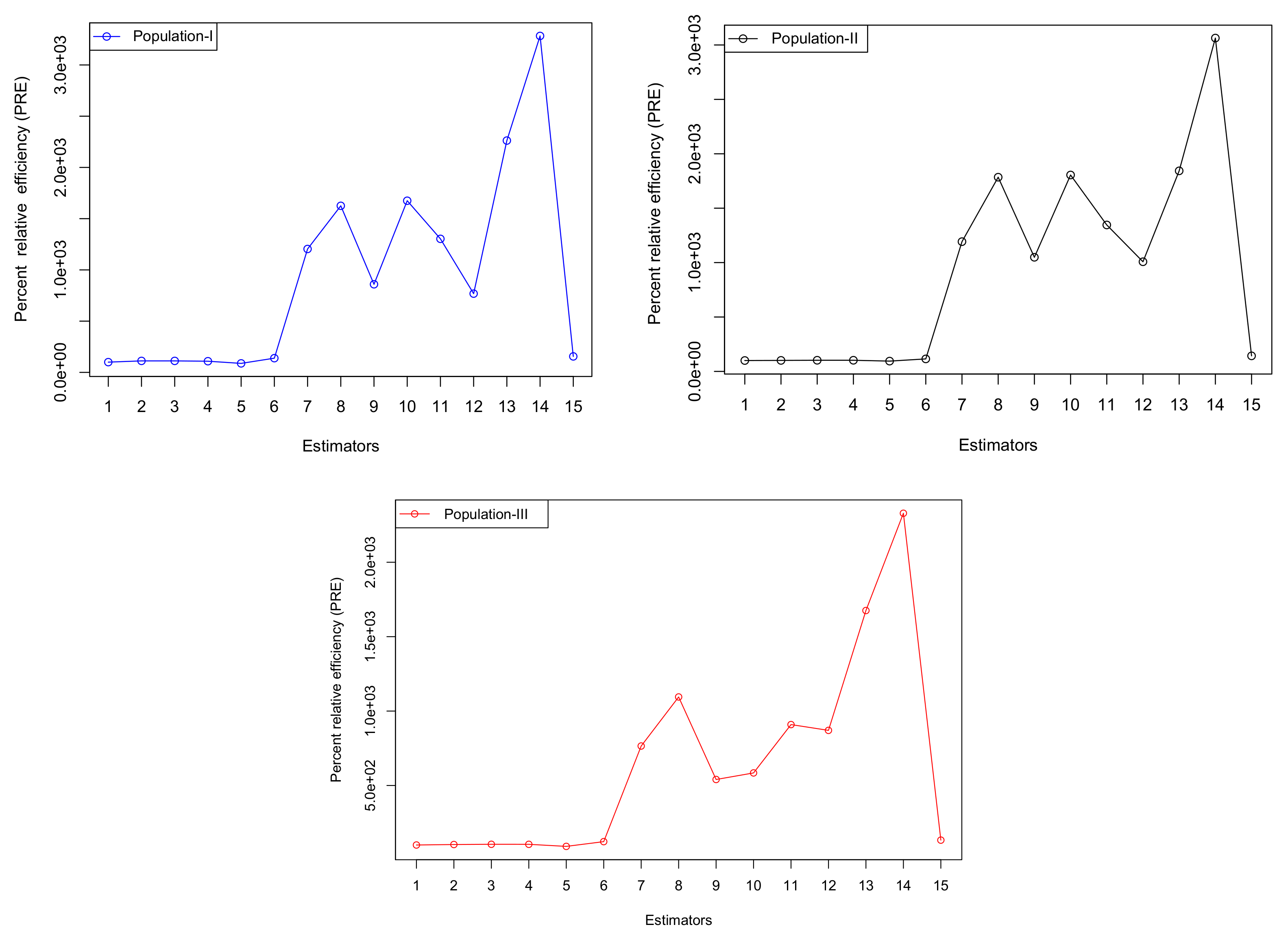
${\theta }_2$	0.14	0.14	0.14	${\theta }_3$	0.04	0.04	0.04

, while the comparison of percent relative efficiency (PRE) values between the newly proposed estimators and the existing ones is presented in Table 5.

6.3. Discussion

Simulation studies and analysis of three real populations were conducted to evaluate the performance of the proposed estimators. The estimators were compared using the percent relative efficiency (PRE) criterion. Table 4 shows the simulation results, including PRE values for both proposed and existing estimators, while Table 5 summarizes the findings from the real populations. The following general conclusions can be drawn from these studies:

• All simulated scenarios and real datasets show that the $PRE$ values for all suggested estimators are higher than those of the existing estimators reported in the literature, as shown in Table 4 and Table 5. This demonstrates how well the suggested estimators perform in comparison to the existing ones.
• In addition, all suggested estimators have $PRE$ values that are consistently higher than those of existing estimators, as demonstrated by the upward-trending graph lines in Figure 1 and Figure 2 for both simulation studies and real populations. This suggests that the suggested classes of estimators perform better than the existing ones, as evidenced by the inverse relationship between the $PRE$ values for the suggested and existing estimators.

Table 4. PRE of different estimators using the artificial populations.

Estimator	$\mathit{L}\mathit{N}(7,4)$	$\mathit{L}\mathit{N}(9,6)$	$\mathit{E}\mathit{x}\mathit{p}\left(4\right)$	$\mathit{E}\mathit{x}\mathit{p}\left(9\right)$	$\mathit{G}\mathit{a}\mathit{m}(3,5)$	$\mathbf{Gam}(7,10)$
${\widehat{Q}}_1$	100	100	100	100	100	100
${\widehat{Q}}_2$	105.839	107.971	108.983	110.287	111.064	114.373
${\widehat{Q}}_3$	118.317	120.643	113.286	115.735	127.677	129.607
${\widehat{Q}}_4$	123.695	126.703	122.730	131/398	140.342	146.740
${\widehat{Q}}_5$	91.973	98.514	87.843	93.665	92.081	97.192
${\widehat{Q}}_6$	123.787	126.812l	130.209	134.947	140.556	145.389
${\widehat{T}}_1$	508.112	683.541	576.577	616.447	704.186	818.293
${\widehat{T}}_2$	974.074	1046.103	783.673	830.248	952.000	1035.902
${\widehat{T}}_3$	423.399	559.205	530.387	569.895	619.075	691.546
${\widehat{T}}_4$	1295.076	1331.667	807.595	844.140	1028.387	1102.939
${\widehat{T}}_5$	1057.236	1203.164	784.793	847.426	1068.354	1178.732
${\widehat{T}}_6$	393.263	583.854	539.394	589.307	673.846	720.480
${\widehat{T}}_7$	1349.529	1559.195	1082.609	1132.379	1108.818	1266.757
${\widehat{T}}_8$	1610.804	1793.650	1206.316	1476.295	1310.380	1420.820
${\widehat{T}}_e$	169.632	175.107	147.969	173.367	181.864	197.643

Table 4. PRE of different estimators using the artificial populations.

Estimator	$\mathit{L}\mathit{N}(7,4)$	$\mathit{L}\mathit{N}(9,6)$	$\mathit{E}\mathit{x}\mathit{p}\left(4\right)$	$\mathit{E}\mathit{x}\mathit{p}\left(9\right)$	$\mathit{G}\mathit{a}\mathit{m}(3,5)$	$\mathbf{Gam}(7,10)$
${\widehat{Q}}_1$	100	100	100	100	100	100
${\widehat{Q}}_2$	105.839	107.971	108.983	110.287	111.064	114.373
${\widehat{Q}}_3$	118.317	120.643	113.286	115.735	127.677	129.607
${\widehat{Q}}_4$	123.695	126.703	122.730	131/398	140.342	146.740
${\widehat{Q}}_5$	91.973	98.514	87.843	93.665	92.081	97.192
${\widehat{Q}}_6$	123.787	126.812l	130.209	134.947	140.556	145.389
${\widehat{T}}_1$	508.112	683.541	576.577	616.447	704.186	818.293
${\widehat{T}}_2$	974.074	1046.103	783.673	830.248	952.000	1035.902
${\widehat{T}}_3$	423.399	559.205	530.387	569.895	619.075	691.546
${\widehat{T}}_4$	1295.076	1331.667	807.595	844.140	1028.387	1102.939
${\widehat{T}}_5$	1057.236	1203.164	784.793	847.426	1068.354	1178.732
${\widehat{T}}_6$	393.263	583.854	539.394	589.307	673.846	720.480
${\widehat{T}}_7$	1349.529	1559.195	1082.609	1132.379	1108.818	1266.757
${\widehat{T}}_8$	1610.804	1793.650	1206.316	1476.295	1310.380	1420.820
${\widehat{T}}_e$	169.632	175.107	147.969	173.367	181.864	197.643

Table 5. PRE of different estimators using real populations.

Estimator	PRE: Pop-I	PRE: Pop-II	PRE: Pop-III
${\widehat{Q}}_1$	100	100	100
${\widehat{Q}}_2$	112.104	101.092	103.252
${\widehat{Q}}_3$	112.106	102.383	104.870
${\widehat{Q}}_4$	108.945	102.342	104.642
${\widehat{Q}}_5$	87.845	94.535	90.71429
${\widehat{Q}}_6$	138.664	114.875	122.651
${\widehat{T}}_1$	1204.266	1192.485	765.188
${\widehat{T}}_2$	1625.500	1784.690	1094.834
${\widehat{T}}_3$	859.653	1048.866	540.278
${\widehat{T}}_4$	1675.141	1805.001	584.391
${\widehat{T}}_5$	1303.178	1345.824	909.167
${\widehat{T}}_6$	768.419	1007.728	870.308
${\widehat{T}}_7$	2262.137	1843.198	1675.656
${\widehat{T}}_8$	3283.4	3063.480	2329.250
${\widehat{T}}_e$	155.795	142.829	132.737

Table 5. PRE of different estimators using real populations.

Estimator	PRE: Pop-I	PRE: Pop-II	PRE: Pop-III
${\widehat{Q}}_1$	100	100	100
${\widehat{Q}}_2$	112.104	101.092	103.252
${\widehat{Q}}_3$	112.106	102.383	104.870
${\widehat{Q}}_4$	108.945	102.342	104.642
${\widehat{Q}}_5$	87.845	94.535	90.71429
${\widehat{Q}}_6$	138.664	114.875	122.651
${\widehat{T}}_1$	1204.266	1192.485	765.188
${\widehat{T}}_2$	1625.500	1784.690	1094.834
${\widehat{T}}_3$	859.653	1048.866	540.278
${\widehat{T}}_4$	1675.141	1805.001	584.391
${\widehat{T}}_5$	1303.178	1345.824	909.167
${\widehat{T}}_6$	768.419	1007.728	870.308
${\widehat{T}}_7$	2262.137	1843.198	1675.656
${\widehat{T}}_8$	3283.4	3063.480	2329.250
${\widehat{T}}_e$	155.795	142.829	132.737

7. Conclusions

This article introduces new classes of efficient estimators for the finite population mean, utilizing the ranks of the auxiliary variable along with the known minimum and maximum values. To assess the properties of these estimators in comparison to existing ones, we derived theoretical conditions in Section 5, demonstrating the improved efficiency of the proposed methods. To verify these conditions, simulation studies and analysis of various empirical datasets were carried out. The results indicate that the proposed estimators consistently outperform the existing ones in terms of percent relative efficiency (PRE), as illustrated in Table 4. These findings are further supported by the empirical results in Table 5, which validate the theoretical conditions established in Section 5.

The simulation results and empirical studies clearly demonstrate that the proposed estimators ${\widehat{T}}_i$$(i=e,1,2,\dots ,8)$ outperform the other estimators under consideration in terms of efficiency. Among the proposed estimators, ${\widehat{T}}_8$ stands out as the most effective choice and is therefore strongly recommended for use.

In addition, our study examined the properties of the proposed efficient estimators within a two-phase sampling framework. Moving forward, there is significant potential to develop new estimators based on these findings, aiming to achieve even higher percent relative efficiency (PRE) values. Future research may focus on extending these estimators to more complex sampling designs, such as stratified or multistage sampling, to evaluate their effectiveness in various practical contexts. Furthermore, the use of machine learning methods for adaptive sampling may offer valuable perspectives on improving estimator efficiency. Exploring the application of these estimators in fields like environmental monitoring or healthcare data analysis can also lead to new opportunities for real-world implementation.

References

- Cochran, W.B. Sampling Techniques; John Wiley and Sons: Hoboken, NJ, USA, 1963. [Google Scholar]
- Khoshnevisan, M.; Singh, R.; Chauhan, P.; Sawan, N. A general family of estimators for estimating population mean using known value of some population parameter (s). Far East J. Theor. Stat. 2007, 22, 181–191. [Google Scholar]
- Rueda, M.M.; Arcos, A.; Martınez-Miranda, M.D.; Román, Y. Some improved estimators of finite population quantile using auxiliary information in sample surveys. Comput. Stat. Data Anal. 2004, 45, 825–848. [Google Scholar] [CrossRef]
- Särndal, C.E. Sample survey theory vs. general statistical theory: Estimation of the population mean. Int. Stat. Rev. Rev. Int. Stat. 1972, 40, 1–12. [Google Scholar] [CrossRef]
- Tarima, S.; Pavlov, D. Using auxiliary information in statistical function estimation. ESAIM Probab. Stat. 2006, 10, 11–23. [Google Scholar] [CrossRef]
- Neyman, J. Contribution to the theory of sampling human populations. J. Am. Stat. Assoc. 1938, 33, 101–116. [Google Scholar] [CrossRef]
- Sukhatme, B.V. Some ratio-type estimators in two-phase sampling. J. Am. Stat. Assoc. 1962, 57, 628–632. [Google Scholar] [CrossRef]
- Erinola, A.Y.; Singh, R.V.K.; Audu, A.; James, T. Modified class of estimator for finite population mean under two-phase sampling using regression estimation approach. Asian J. Probab. Stat. 2021, 4, 52–64. [Google Scholar] [CrossRef]
- Garg, N.; Srivastava, M. A general class of estimators of a finite population mean using multi-auxiliary information under two stage sampling scheme. J. Reliab. Stat. Stud. 2009, 2, 103–118. [Google Scholar]
- Guha, S.; Chandra, H. Improved estimation of finite population mean in two-phase sampling with subsampling of the nonrespondents. Math. Popul. Stud. 2021, 28, 24–44. [Google Scholar] [CrossRef]
- Daraz, U.; Wu, J.; Agustiana, D.; Emam, W. Finite population variance estimation using Monte Carlo simulation and real life application. Symmetry 2025, 17, 84. [Google Scholar] [CrossRef]
- Daraz, U.; Agustiana, D.; Wu, J.; Emam, W. Twofold auxiliary information under two-phase sampling: An improved family of double-transformed variance estimators. Axioms 2025, 14, 64. [Google Scholar] [CrossRef]
- Singh, H.P.; Vishwakarma, G.K. Modified exponential ratio and product estimators for finite population mean in double sampling. Austrian J. Stat. 2007, 36, 217–225. [Google Scholar] [CrossRef]
- Singh, H.P.; Espeio, M.R. Double sampling ratio-product estimator of a finite population mean in sample surveys. J. Appl. Stat. 2007, 34, 71–85. [Google Scholar] [CrossRef]
- Vishwakarma, G.K.; Zeeshan, S.M. Generalized ratio-cum-product estimator for finite population mean under two-phase sampling scheme. J. Mod. Appl. Stat. Methods 2020, 19, 1–16. [Google Scholar] [CrossRef]
- Zaman, T.; Kadilar, C. New class of exponential estimators for finite population mean in two-phase sampling. Commun. Stat.-Theory Methods 2021, 50, 874–889. [Google Scholar] [CrossRef]
- Albalawi, O. Estimation techniques utilizing dual auxiliary variables in stratified two-phase sampling. AIMS Math 2024, 9, 33139–33160. [Google Scholar] [CrossRef]
- Mohanty, S.; Sahoo, J. A note on improving the ratio method of estimation through linear transformation using certain known population parameters. Sankhyā Indian J. Stat. Ser. 1995, 57, 93–102. [Google Scholar]
- Khan, M.; Shabbir, J. Some improved ratio, product, and regression estimators of finite population mean when using minimum and maximum values. Sci. World J. 2013, 2013, 431868. [Google Scholar] [CrossRef]
- Khan, M. Improvement in estimating the finite population mean under maximum and minimum values in double sampling scheme. J. Stat. Appl. Probab. Lett. 2015, 2, 115–121. [Google Scholar]
- Walia, G.S.; Kaur, H.; Sharma, M. Ratio type estimator of population mean through efficient linear transformation. Am. J. Math. Stat. 2015, 5, 144–149. [Google Scholar]
- Daraz, U.; Shabbir, J.; Khan, H. Estimation of finite population mean by using minimum and maximum values in stratified random sampling. J. Mod. Appl. Stat. Methods 2018, 17, 1–15. [Google Scholar] [CrossRef]
- Daraz, U.; Khan, M. Estimation of variance of the difference-cum-ratio-type exponential estimator in simple random sampling. Res. Math. Stat. 2021, 8, 1899402. [Google Scholar] [CrossRef]
- Daraz, U.; Wu, J.; Albalawi, O. Double exponential ratio estimator of a finite population variance under extreme values in simple random sampling. Mathematics 2024, 12, 1737. [Google Scholar] [CrossRef]
- Alghamdi, A.S.; Alrweili, H. A comparative study of new ratio-type family of estimators under stratified two-phase sampling. Mathematics 2025, 13, 327. [Google Scholar] [CrossRef]
- Alghamdi, A.S.; Alrweili, H. New class of estimators for finite population mean under stratified double phase sampling with simulation and real-life application. Mathematics 2025, 13, 329. [Google Scholar] [CrossRef]
- Cekim, H.O.; Cingi, H. Some estimator types for population mean using linear transformation with the help of the minimum and maximum values of the auxiliary variable. Hacet. J. Math. Stat. 2017, 46, 685–694. [Google Scholar]
- Alomair, M.A.; Daraz, U. Dual transformation of auxiliary variables by using outliers in stratified random sampling. Mathematics 2024, 12, 2829. [Google Scholar] [CrossRef]
- Daraz, U.; Alomair, M.A.; Albalawi, O.; Al Naim, A.S. New techniques for estimating finite population variance using ranks of auxiliary variable in two-stage sampling. Mathematics 2024, 12, 2741. [Google Scholar] [CrossRef]
- Chatterjee, S.; Hadi, A.S. Regression Analysis by Example; John Wiley & Sons: Hoboken, NJ, USA, 2013. [Google Scholar]
- Daraz, U.; Wu, J.; Alomair, M.A.; Aldoghan, L.A. New classes of difference cum-ratio-type exponential estimators for a finite population variance in stratified random sampling. Heliyon 2024, 10, e33402. [Google Scholar] [CrossRef]
- Daraz, U.; Alomair, M.A.; Albalawi, O. Variance estimation under some transformation for both symmetric and asymmetric data. Symmetry 2024, 16, 957. [Google Scholar] [CrossRef]
- Bureau of Statistics. Punjab Development Statistics; Government of the Punjab: Lahore, Pakistan, 2013.