Abstract
This paper introduces a novel three-dimensional financial risk system that exhibits complex dynamical behaviors, including chaos, multistability, and a butterfly attractor. The proposed system is an extension of the Zhang financial risk model (ZFRM), with modifications that enhance its applicability to real-world economic stability assessments. Through numerical simulations, we confirm the system’s chaotic nature using Lyapunov exponents (LE), with values calculated as , indicating a positive Maximal Lyapunov Exponent (MLE) that confirms chaos. The Kaplan–Yorke Dimension (KYD) is determined as Dk = 2.1575, reflecting the system’s fractal characteristics. Bifurcation analysis (BA) reveals parameter ranges where transitions between periodic, chaotic, and multistable states occur. Additionally, the system demonstrates coexisting attractors, where different initial conditions lead to distinct long-term behaviors, emphasizing its sensitivity to market fluctuations. Offset Boosting Control (OBC) is implemented to manipulate the chaotic attractor, shifting its amplitude without altering the underlying system dynamics. These findings provide deeper insights into financial risk modeling and economic stability, with potential applications in financial forecasting, risk assessment, and secure economic data transmission.
MSC:
34C23; 65P20
1. Introduction
A country’s Financial Risk Models (FRMs) significantly impact its GDP by influencing investment, consumption, and overall economic stability [1,2]. A high FRM, such as market volatility, credit instability, or banking crises, can reduce investor confidence, leading to lower capital inflows and decreased business expansion [3,4]. This, in turn, affects employment rates and household spending, key drivers of GDP growth. Additionally, financial instability can lead to higher borrowing costs for governments and businesses, reducing public- and private-sector investments in infrastructure and innovation [5,6]. In contrast, effective FRM management enhances economic resilience, stabilizing currency values and fostering sustainable GDP growth. Thus, understanding and mitigating the FRM is crucial for maintaining economic stability and long-term prosperity [7,8].
Studying chaotic systems in FRM and economic analysis is crucial for countries because financial markets and economic systems often exhibit nonlinear, unpredictable behavior influenced by numerous interconnected factors [9,10]. Chaos theory helps in understanding how small fluctuations in economic variables, such as interest rates, inflation, or market sentiment, can lead to significant and unexpected consequences, impacting national and global economies [11,12]. By analyzing chaotic behavior in FRMs, policy makers and financial institutions can better anticipate crises, design more resilient economic policies, and implement effective risk mitigation strategies [13,14]. Moreover, chaotic models aid in forecasting economic trends more accurately than traditional linear models, helping countries manage uncertainties, optimize resource allocation, and ensure sustainable economic growth [15].
The development of chaotic systems in FRMs has evolved as a powerful tool for understanding the unpredictable and nonlinear nature of financial markets [16]. Early financial models were primarily based on deterministic and linear equations, but real-world economic systems exhibit complex behaviors that cannot be captured by traditional methods [17]. Researchers began integrating chaos theory into FRMs, starting with models such as the Lorenz and Rössler systems, which demonstrated sensitive dependence on initial conditions [18,19,20]. The introduction of the ZFRM marked a significant step in applying chaos theory to economic stability assessment. Over time, modifications to these models, including the incorporation of additional nonlinear terms, time delays, and multistability phenomena, have improved their applicability.
In financial markets, multistability can lead to sudden and unpredictable transitions between stable economic phases, such as growth, recession, or crisis, depending on external shocks or investor sentiment [21,22]. This phenomenon poses challenges for risk assessment and market stability, as small perturbations can push the system into drastically different financial conditions. In economic models, multistability influences policy-making, as governments and central banks must design robust strategies to avoid unwanted state transitions that could lead to prolonged financial instability [23]. For instance, improper fiscal or monetary interventions could unintentionally shift an economy from a stable growth phase to a recessionary state. Regarding GDP, multistability can result in fluctuating economic performance, where economies may experience rapid growth, stagnation, or crisis based on initial economic conditions and external influences [24,25].
In recent years, the financial literature has shown growing interest in the modeling of chaotic systems. Pei and Sun [26] analyze the intricate dynamics of a time-delayed FRM, focusing on rich behavior such as quasi-periodic, phase-locked, and chaotic solutions that significantly impact financial stability. Also, they identified double Hopf bifurcation points and derived critical curves of Hopf bifurcation to understand their effects on system dynamics. Moualkia et al. [27] discussed a chaotic FRM by designing feedback controllers in both stochastic and fractional cases, addressing the impact of external disturbances often overlooked in deterministic approaches. Musaev and Grigoriev [28] investigated the stability and feasibility of trend management strategies under stochastic chaos conditions, particularly in speculative Forex trading. They evaluated the robustness of these strategies for asset management through sequential optimization and testing across three EURUSD observation intervals, alternating between training and testing phases. Johansyah et al. [29] investigated the dynamics and control of a newly proposed chaotic monetary system characterized by transient chaos. The system is modeled using an autonomous set of absolute nonlinearity equations, exhibiting chaotic behavior under specific parameter conditions [30].
Foroni and Gardini [31] analyzed a class of heterogeneous market models and studied the homoclinic bifurcations associated with the chaotic attractors in the heterogeneous market models. Mihailescu [32] investigated the metric, ergodic, and stability properties of certain implicitly defined economic models such as 1-D and 2-D overlapping generations models, a cash-in-advance model, heterogeneous markets and a cobweb model. Zhang [33] applied nonlinear difference equations to study periodic, aperiodic, or chaotic behavior of several economic models.
Based on the above literature, most FRMs do not incorporate mechanisms for controlling chaotic behavior in a way that allows dynamic adjustments without altering the system’s fundamental properties. Furthermore, while some works address FRM stability, they rarely analyze the sensitivity of an FRM to initial conditions or examine multistability in the context of economic stability assessment. This paper fills these gaps by introducing a new three-dimensional financial risk system with a butterfly attractor, performing an in-depth analysis of its chaotic properties, and implementing OBC to manipulate chaotic signals.
The main contribution and novelty of this paper as follows:
- This paper introduces a new three-dimensional FRM that extends the ZFRM by incorporating a butterfly attractor. The proposed model captures complex market dynamics and improves economic stability assessment.
- The study analyzes the system’s chaotic behavior, producing LE1 = 0.8972, LE2 = 0.0000, LE3 = −1.3421) and DKY = 2.668). It explores bifurcation patterns, coexisting attractors, and sensitivity to initial conditions, providing deeper insights into FRMs.
- The paper introduces an OBC mechanism to manipulate the chaotic attractor’s amplitude without altering the system’s core dynamics.
This paper is structured as follows: Section 1 discusses the importance of financial risk modeling and the role of chaotic systems in understanding economic stability. Section 2 introduces the proposed three-dimensional financial risk system, extending the Zhang model and incorporating a butterfly attractor. Section 3 presents a detailed dynamical analysis and the influence of key system parameters on equilibrium, periodicity, and chaos. In addition, we discuss how offset boosting is applied to manipulate the chaotic attractor. Finally, Section 4 summarizes key findings and suggests directions for further research in financial risk modeling and nonlinear economic systems.
2. Mathematical Model of Financial System
In 2013, Zhang et al. [30] proposed a 3-D FRM dynamical system, which is described as follows:
In the ZFRM (1), , and represent occurrence value risk, analysis value risk, and control value risk in the current market, respectively. We use the notation It is also reported in [30] that is the analysis risk efficiency, is the transmission rate of the previous risk, and where represents the distortion coefficient of risk control. It was noted in [30] that the ZFRM (1) is closer to the actual situation of the risk management process in the financial market, where the occurrence of current risk is decided by the previous risk analysis result and the previous risk control to risk analysis.
It was reported in [30] that the ZFRM (1) exhibits a chaotic attractor for the parameter values chosen as , and The Zhang financial risk system (1) is very similar to the famous Lorenz weather chaotic system [34]; the only difference is the quadratic nonlinearity in the first differential equation for the Zhang dynamical system (1). Indeed, the Lorenz weather chaotic system (LWCS) is given by the 3-D dynamics
For the initial state we computed the LE for the ZFRM (1) for s using the Wolf Algorithm [35] and obtained the following result:
Using the LE values in Equation (2), we can compute the KYD for the ZFRM (1) as follows:
Thus, the ZFRM (1) is a dissipative chaotic system with the MLE equal to and KYD equal to .
For the initial state we computed the LE for the LWCS (2) for s using the Wolf Algorithm [35] and obtained the following result:
Using the LE values in Equation (4), we can compute the KYD for the LWCS (2) as follows:
Thus, the LWCS (2) is a dissipative chaotic system with the MLE equal to and KYD equal to .
In this research work, we propose a new FRM by modifying the dynamics of the ZFRM (1). Explicitly, we add a sinusoidal nonlinearity, in the second differential equation for the ZFRM (1), which accounts for the risk fluctuations in the financial market. We also consider different parameter values for our FRM. In the development of the Financial Risk System with Butterfly Attractors (FRSBA), the term +p·sin(x) is introduced in the second equation to represent periodic and unpredictable fluctuations in market risk. Economically, financial markets are not solely influenced by deterministic factors such as interest rates or exchange rates, but also by psychological elements and investor sentiment, which often exhibit cyclical and reactive behavior in response to external stimuli.
The term sin(x) captures this periodic nature, where x, representing the occurrence value risk, undergoes oscillatory fluctuations due to feedback from prior risk events. The coefficient p acts as an amplification factor, indicating the market’s sensitivity to these oscillations. By incorporating this sinusoidal nonlinearity, the model is better equipped to simulate real-world market dynamics, where investor behavior and market reactions often lead to volatility spikes, sentiment-driven rallies, or panic selling, none of which can be fully captured by purely linear or deterministic models. Thus, the +p·sin(x) term enhances the model’s ability to account for risk feedback loops and cyclical irrational behavior, making it more robust for economic stability analysis and financial risk forecasting.
Thus, we propose the following Financial Risk System with Butterfly Attractors (FRSBA):
We represent the state of the FRSBA (7) as The states and the modelling constants have the same financial interpretation as in the ZFRM (1). In the new model FRSBA (7), is a positive constant and the nonlinear term denotes the risk fluctuation in the financial market.
In the new model FRSBA (7), x, y, and z represent occurrence value risk, analysis value risk, and control value risk in the current market, respectively. It is well known that is a periodic trigonometric function that oscillates with a period of and bounded between the values and When the value of is small, the sinusoidal nonlinearity represents the risk fluctuation in the occurrence value risk in the financial market.
We shall show that the FRSBA (7) has a chaotic attractor for the parameter values and We take the initial state as For s and the LE for the FRSBA (7) was found using the Wolf Algorithm [34] as follows:
Using the LE values in Equation (8), we can compute the KYD for the FRSBA (7) as follows:
Table 1 gives a comparison of the MLE and KYD between the ZFRM [30], LWCS [34], and the FRSBA (4) in this work.

Table 1.
Comparison table—ZFRM [30], LWCS [34], and the FRSBA.
3. Sensitivity Analysis of System Dynamics, Multistability, and Offset Boosting
In this part, we conduct a comprehensive sensitivity analysis of the proposed financial system’s dynamics, focusing on how its parameters and initial conditions influence its behavior. Utilizing key analytical tools such as bifurcation diagrams, phase portraits, and the Lyapunov exponent spectrum, we delve into the system’s intricate properties. This section contains the sensitivity analysis of the new financial system, which considers a broad range of parameter variations and their combined effects. Specifically, we have considered broad ranges such as the range for the parameter the range for the parameter the range for the parameter and for the parameter This investigation allows us to pinpoint regions where chaotic behavior and multistability emerge, alongside other noteworthy phenomena such as offset boosting. Multistability is a special feature in the nonlinear dynamical systems, and it alludes to the phenomenon in dynamical systems where a system can coexist in multiple distinct stable states or attractors under the same set of governing parameters but varying values of the initial conditions [35]. Offset boosting control for the nonlinear dynamical systems modifies one of the states, say by introducing an offset or a bias in the state and replacing the state by to improve the performance of the underlying nonlinear dynamical system. Offset boosting control is a useful technique in the study of chaotic dynamical systems [36]. All the numerical simulations in this section have been carried out using MATLAB R2024b software.
3.1. Influence of Parameter a on Equilibrium, Periodicity, and Chaos
The impact of parameter a on the system’s behavior is examined by varying its value from 1 to 15. Using the BA and LE shown in Figure 1a,b, different dynamic patterns are identified. When a is in the range [1, 3.6], the system’s trajectories settle at equilibrium points, as indicated by a negative MLE in Figure 1b. This is further illustrated in Figure 1c, which presents a trajectory plot when . In the intervals [3.6, 8.5] and [9.7, 10.3], the system exhibits periodic behavior, confirmed by a zero MLE in Figure 1b. Figure 1a provides additional evidence of this periodicity, while Figure 1d visually represents the periodic attractor when a = 5. When a falls within [8.5, 9.7] or [10.3, 15], the system shows chaotic behavior, except for two periodic windows occurring at and . This chaotic behavior is further illustrated in Figure 1e, which depicts the chaotic attractor when
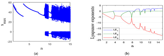
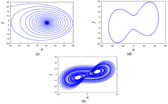
Figure 1.
(a) BA, (b) LEs, (c) x-y stable state for a = 2, (d) x-y periodic attractor for a = 5, and (e) x-y chaotic attractor for a = 13.
The presence of chaos and periodicity in an FRM can significantly impact risk and efficiency. When an FRM exhibits chaotic behavior, small changes in initial conditions can lead to vastly different outcomes, making prediction and risk assessment highly challenging. This unpredictability increases market volatility, reduces investor confidence, and complicates the implementation of risk management strategies. On the other hand, periodic behavior in an FRM can provide some level of predictability, but it may also lead to cycles of boom and bust, where efficiency is periodically disrupted by extreme fluctuations in market conditions.
From an efficiency perspective, chaos can lead to inefficiencies in capital allocation and pricing mechanisms, as FRMs struggle to accurately capture future market movements. In contrast, periodic behavior might allow for better forecasting in the short term, but it can also create systemic vulnerabilities if market participants rely too heavily on predictable cycles. When chaos and periodicity coexist, an FRM may alternate between stability and instability, necessitating adaptive risk management approaches. This interplay underscores the importance of robust financial policies and machine learning-driven predictive models to mitigate risks and enhance system resilience.
3.2. Influence of Parameter b on Equilibrium, Periodicity, and Chaos
The effect of parameter on the system’s dynamics is analyzed by varying its value between 3 and 15. According to the BA and LE in Figure 2a,b, different behaviors emerge. When b is within [3, 5.1] or [5.3, 12.4], the system exhibits chaotic behavior, except for a periodic window at . This chaotic state is illustrated in Figure 2c, which shows the attractor when . In the interval [5.1, 5.3], the system transitions to periodic behavior, verified by a zero MLE in Figure 2b. Additional confirmation is provided by Figure 2a, while Figure 2d depicts the periodic attractor for . When is in the range [12.4, 15], the system stabilizes at equilibrium points, as indicated by a negative MLE in Figure 2b. This stabilization is further visualized in Figure 2e, which illustrates the trajectory when .
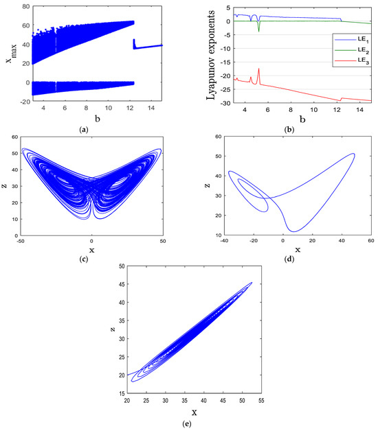
Figure 2.
(a) BA, (b) LE, (c) x-z chaotic behavior for b = 4, (d) x-z periodic attractor for b = 5.2, (e) x-y stable state for b = 14.
The distortion coefficient of risk control in an FRM exhibiting chaos and periodicity significantly affects the system’s stability, risk mitigation efficiency, and overall financial resilience. In a chaotic FRM, a high distortion coefficient can amplify the unpredictability of risk dynamics, leading to greater market volatility. When risk control mechanisms are highly distorted, their effectiveness in stabilizing financial fluctuations diminishes, making it harder for policy makers and investors to anticipate and manage risks. This can result in erratic financial behavior, where small miscalculations in risk control policies trigger large-scale economic instability, increasing the likelihood of financial crises, speculative bubbles, or abrupt market crashes.
On the other hand, in an FRM with periodic behavior, the distortion coefficient influences how consistently risk control measures interact with predictable market cycles. A moderate distortion coefficient may introduce controlled fluctuations that allow for adaptive adjustments to financial policies, improving long-term stability. However, excessive distortion can disrupt the periodic nature of the system, causing unexpected shifts between stable and unstable states. This transition between chaos and periodicity complicates financial forecasting and risk assessment, requiring more sophisticated control mechanisms, such as machine learning-driven optimization and adaptive economic policies. Therefore, managing the distortion coefficient effectively is crucial in maintaining financial stability, minimizing systemic risks, and enhancing the robustness of financial decision-making.
3.3. Influence of Parameter c on Periodicity and Chaos
The effect of parameter on the system’s behavior is analyzed by varying its value between 30 and 100. Figure 3a,b present the BA and LE, respectively, highlighting different dynamical behavior. When c falls within [30, 52] or [55, 71], the system exhibits chaotic dynamics, except for two periodic windows at , and . This is confirmed by Figure 3b, where the MLE is positive in these ranges. A visualization of the chaotic attractor for is shown in Figure 3c. For c within [52, 55] or [71, 100], the system transitions to periodic behavior, as indicated in Figure 3a. This periodicity is further validated by a zero MLE in Figure 3b. Additionally, Figure 3d illustrates the periodic attractor corresponding to .
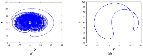
Figure 3.
(a) BA, (b) LE, (c) y-z chaotic attractor for c = 60, (d) y-z periodic attractor for c = 80.
The transmission rate of previous risk in an FRM exhibiting chaos and periodicity plays a crucial role in risk propagation and stability. When the system is chaotic, small variations in past risks can amplify unpredictably, leading to erratic financial behavior. This high sensitivity means that even minor financial shocks can have disproportionately large effects on market stability, making risk management more challenging. The chaotic nature of such a system results in periods of extreme volatility, where risk transmission can escalate rapidly, reducing the effectiveness of traditional risk mitigation strategies and increasing systemic instability.
On the other hand, if the FRM exhibits periodic behavior, the transmission of previous risks follows a more structured pattern. This periodicity allows financial institutions to anticipate risk cycles, potentially mitigating adverse effects through strategic interventions. However, periodic transmission also creates vulnerabilities, as financial entities may become overly reliant on expected cycles, failing to prepare for unexpected disruptions. The coexistence of chaos and periodicity complicates risk forecasting, as the system may shift unpredictably between stable and unstable phases.
3.4. Influence of Parameter p on Equilibrium and Chaos
The influence of parameter on the system’s behavior is examined by varying its value from 0 to 30. Figure 4a,b display the BA and LE, revealing distinct dynamic patterns. Within the range [0, 22.5], the system demonstrates chaotic behavior, confirmed by a positive MLE. This chaotic nature is illustrated in Figure 4c, which presents the attractor for . As p increases beyond 22.5 up to 30, the system transitions to a stable equilibrium, as evidenced by a negative MLE in Figure 4b. This stabilization is further depicted in Figure 4d, showing the trajectory for .
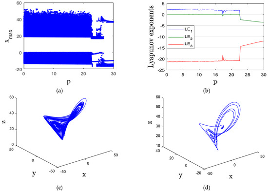
Figure 4.
(a) BA, (b) LE, (c) x-y-z chaotic attractor for , (d) x-y-z periodic attractor for .
Risk fluctuations in a financial market that exhibits both chaos and periodicity can have profound implications for market stability and economic decision-making. In a chaotic FRM, risk fluctuations become highly unpredictable due to the system’s sensitivity to initial conditions. Small disturbances in market conditions, such as changes in interest rates, investor sentiment, or geopolitical events, can lead to disproportionate financial swings. This unpredictability increases market volatility, making it difficult for investors and policy makers to implement effective risk management strategies. As a result, financial markets may experience sudden crashes, liquidity shortages, or speculative bubbles that destabilize economic growth.
Conversely, in an FRM exhibiting periodicity, risk fluctuations tend to follow identifiable cycles, allowing market participants to anticipate financial upswings and downturns. While this structured behavior provides a degree of predictability, it also introduces systemic risks if market actors rely too heavily on expected cycles. If an unexpected event disrupts the periodic pattern, it can trigger widespread uncertainty and financial instability. The interplay between chaos and periodicity further complicates risk assessment, as markets may transition unpredictably between stable and unstable states.
3.5. Influence of Initial Conditions on Chaos and Multistability
This section explores the impact of initial conditions on the system, emphasizing multistability and the presence of distinct chaotic attractors that emerge under the same parameter values but different starting points.
Multistability is a special feature in the nonlinear dynamical systems, and it alludes to the phenomenon in dynamical systems where a system can coexist in multiple distinct stable states or attractors under the same set of governing parameters but varying values of the initial conditions [36].
To demonstrate the multistability phenomenon, two initial states are considered: [20, 20, 20] (represented in blue) and [20, 20, −20] (represented in red). A bifurcation diagram is generated for System (1) by varying parameter c from 65 to 100. As illustrated in Figure 5, the system exhibits both coexisting chaotic and periodic attractors.
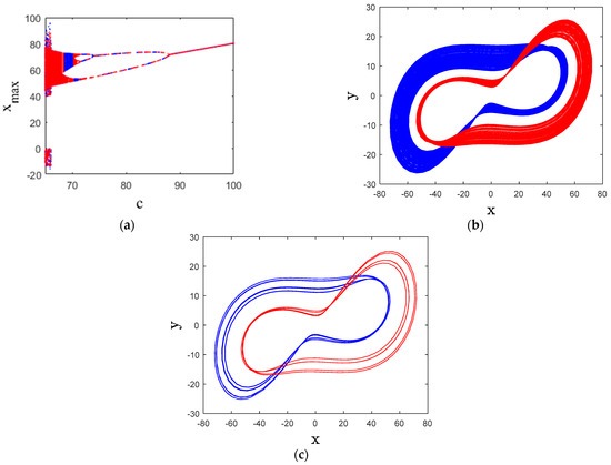
Figure 5.
(a) BA, (b) two coexisting chaotic attractors for , (c) two coexisting periodic attractors for .
3.6. Offset Boosting Control for Attractor Adjustment
Offset Boosting Control (OBC) is an effective technique for modifying a system’s amplitude by integrating a feedback state [37]. While it does not alter the system’s fundamental dynamics, it enables shifting the attractor’s position in either direction based on the control parameter. In the newly introduced 3D system, chaotic behavior with adjustable boosting is observed, particularly affecting .
By replacing with in the equations of the new system FRSBA (4), we obtain
The amplitude of the state z of the new system (10) can be modified, as illustrated by the z-x attractor in Figure 6. A negative shifts the attractor positively, while a positive results in a negative displacement. This mechanism allows the chaotic signal to transition from bipolar to unipolar, offering significant potential for the proposed financial system in secure communications and engineering applications.
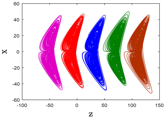
Figure 6.
z-x chaotic attractors of (7) for different values of offset boosting parameter: k = 0 (blue), k = 40 (red), k = −40 (green), k = 80 (magenta), and k = −80 (brown).
4. Conclusions
In this paper, a novel FRSBA was introduced to analyze complex market dynamics and economic stability. BA demonstrated transitions between periodic, chaotic, and stable states, providing insights into financial risk fluctuations. Additionally, the implementation of offset boosting control allowed for effective manipulation of chaotic signals without altering the system’s core structure, offering potential applications in financial forecasting, risk assessment, and secure communication. The findings of this study contribute to a deeper understanding of chaotic FRMs, emphasizing the need for robust risk management strategies in economic decision-making. Future research could explore the integration of machine learning techniques to further optimize financial stability predictions and adaptive control mechanisms for real-world applications. Future research could also consider empirical studies on financial risk models and other applications such as risk assessment and secure communication scenarios. Moreover, stochastic modelling and robustness analysis of financial chaotic systems can be explored as future research studies.
Author Contributions
Conceptualization, M.D.J., S.V. and A.S.; Software, S.V. and K.B.; Validation, E.R.; Formal analysis, C.A., S.K.A., E.R. and A.K.; Investigation, K.B.; Resources, C.A., S.K.A., E.R. and A.K.; Data curation, S.K.A.; Writing—original draft, M.D.J., S.V. and K.B.; Writing—review & editing, A.S. and A.K.; Supervision, M.D.J. and A.S.; Project administration, C.A. All authors have read and agreed to the published version of the manuscript.
Funding
The author thanks to the Rector of Universitas Padjadjaran and the Director of the Directorate Research and Community Service at Universitas Padjadjaran who provideds funds for this project. This work was funded by Universitas Padjadjaran through Riset Kompetensi Dosen Unpad (RKDU) with contract number 4586/UN6.D/PT.00/2025.
Data Availability Statement
The original contributions presented in this study are included in the article. Further inquiries can be directed to the corresponding author.
Conflicts of Interest
The authors declare no conflict of interest.
References
- Patro, D.K.; Wald, J.K.; Wu, Y. The impact of macroeconomic and financial variables on market risk: Evidence from international equity returns. Eur. Financ. Manag. 2002, 8, 421–447. [Google Scholar] [CrossRef]
- Saidi, K. Foreign direct investment, financial development and their impact on the GDP growth in low-income countries. Int. Econ. J. 2018, 32, 483–497. [Google Scholar] [CrossRef]
- Cubillas, E.; Ferrer, E.; Suárez, N. Does investor sentiment affect bank stability? International evidence from lending behavior. J. Int. Money Financ. 2021, 113, 102351. [Google Scholar] [CrossRef]
- Pholphirul, P. Financial Instability, Banking Crisis, and Growth Volatility In Thailand: An Investigation of Bi-Directional Relationship. Int. J. Bus. Manag. 2008, 3, 97–110. [Google Scholar] [CrossRef][Green Version]
- Musau, S.; Muathe, S.; Mwangi, L. Financial inclusion, GDP and credit risk of commercial banks in Kenya. Int. J. Econ. Financ. 2018, 10, 181. [Google Scholar] [CrossRef]
- Vassalou, M. News related to future GDP growth as a risk factor in equity returns. J. Financ. Econ. 2003, 68, 47–73. [Google Scholar] [CrossRef]
- Ozili, P.K.; Iorember, P.T. Financial stability and sustainable development. Int. J. Financ. Econ. 2024, 29, 2620–2646. [Google Scholar] [CrossRef]
- Olawale, A. Capital adequacy and financial stability: A study of Nigerian banks’ resilience in a volatile economy. GSC Adv. Res. Rev. 2024, 21, 001–012. [Google Scholar] [CrossRef]
- Farman, M.; Nisar, K.S.; Ali, M.; Ahmad, H.; Tabassum, M.F.; Ghaffari, A.S. Chaos and forecasting financial risk dynamics with different stochastic economic factors by using fractional operator. Model. Earth Syst. Environ. 2025, 11, 146. [Google Scholar] [CrossRef]
- Gao, X.L.; Li, Z.Y.; Wang, Y.L. Chaotic dynamic behavior of a fractional-order financial system with constant inelastic demand. Int. J. Bifurc. Chaos 2024, 34, 2450111. [Google Scholar] [CrossRef]
- Wu, J.; Xia, L. Double well stochastic resonance for a class of three-dimensional financial systems. Chaos Solitons Fractals 2024, 181, 114632. [Google Scholar] [CrossRef]
- Almaghrebi, Y.S.; Raslan, K.R.; Abd El Salam, M.A.; Ali, K.K. A novel fractal-fractional approach to modeling and analyzing chaotic financial system. Res. Math. 2025, 12, 2468528. [Google Scholar] [CrossRef]
- Olayiwola, M.O.; Alaje, A.I.; Yunus, A.O. A Caputo fractional order financial mathematical model analyzing the impact of an adaptive minimum interest rate and maximum investment demand. Results Control Optim. 2024, 14, 100349. [Google Scholar] [CrossRef]
- Asadollahi, M.; Padar, N.; Fathollahzadeh, A.; Mirzaei, M.J.; Aslmostafa, E. Fixed-time terminal sliding mode control with arbitrary convergence time for a class of chaotic systems applied to a nonlinear finance model. Int. J. Dyn. Control 2024, 12, 1874–1887. [Google Scholar] [CrossRef]
- Tian, Y.; Wu, Y. Systemic Financial Risk Forecasting: A Novel Approach with IGSA-RBFNN. Mathematics 2024, 12, 1610. [Google Scholar] [CrossRef]
- Peng, Y.; de Moraes Souza, J.G. Chaos, overfitting and equilibrium: To what extent can machine learning beat the financial market? Int. Rev. Financ. Anal. 2024, 95, 103474. [Google Scholar] [CrossRef]
- Woode, J.K.; Assifuah-Nunoo, E.; Adjei, A.F.; Bambir, J.; Esuako, A.B. Effect of Investment Knowledge on Investment Decision amid COVID-19 Pandemic: The Moderating Role of Financial Risk Tolerance. Univers. J. Account. Financ. 2024, 12, 60–77. [Google Scholar] [CrossRef]
- Wu, J.; Pan, X.; Wu, K.; Wang, X. Realizing stochastic fixed-time synchronization between two nonlinear chaotic finance systems. Int. J. Mod. Phys. C 2024, 35, 2450040. [Google Scholar] [CrossRef]
- Johansyah, M.D.; Sambas, A.; Farman, M.; Vaidyanathan, S.; Zheng, S.; Foster, B.; Hidayanti, M. Global mittag-leffler attractive sets, boundedness, and finite-time stabilization in novel chaotic 4d supply chain models with fractional order form. Fractal Fract. 2024, 8, 462. [Google Scholar] [CrossRef]
- Alhebri, A. Safeguarding Financial Integrity with Interval-Valued Neutrosophic Analytic Hierarchy Process for Sustainable Accounting Systems. Int. J. Neutrosophic Sci. (IJNS) 2024, 23, 337–345. [Google Scholar]
- Dehingia, K.; Boulaaras, S.; Hinçal, E.; Hosseini, K.; Abdeljawad, T.; Osman, M.S. On the dynamics of a financial system with the effect financial information. Alex. Eng. J. 2024, 106, 438–447. [Google Scholar] [CrossRef]
- Johansyah, M.D.; Sambas, A.; Mobayen, S.; Vaseghi, B.; Al-Azzawi, S.F.; Sukono; Sulaiman, I.M. Dynamical analysis and adaptive finite-time sliding mode control approach of the financial fractional-order chaotic system. Mathematics 2022, 11, 100. [Google Scholar] [CrossRef]
- Ma, R.R.; Wu, J.; Wu, K.; Pan, X. Adaptive fixed-time synchronization of Lorenz systems with application in chaotic finance systems. Nonlinear Dyn. 2022, 109, 3145–3156. [Google Scholar] [CrossRef]
- Lei, Y.; Hou, Q.; Tong, Z. Research on supply chain financial risk prevention based on machine learning. Comput. Intell. Neurosci. 2023, 2023, 6531154. [Google Scholar] [CrossRef]
- Vogl, M.; Roetzel, P.G. Chaoticity versus stochasticity in financial markets: Are daily S&P 500 return dynamics chaotic? Commun. Nonlinear Sci. Numer. Simul. 2022, 108, 106218. [Google Scholar]
- Pei, L.; Sun, M. Quasi-Periodic, Phase-Locked and Chaotic Solutions in a Financial System with Two Feedback Delays. J. Vib. Eng. Technol. 2025, 13, 80. [Google Scholar] [CrossRef]
- Moualkia, S.; Liu, Y.; Cao, J. Stabilization by feedback control of a novel stochastic chaotic finance model with time-varying fractional derivatives. Alex. Eng. J. 2025, 112, 496–509. [Google Scholar] [CrossRef]
- Musaev, A.; Grigoriev, D. The Stability of Trend Management Strategies in Chaotic Market Conditions. J. Risk Financ. Manag. 2025, 18, 33. [Google Scholar] [CrossRef]
- Johansyah, M.D.; Sambas, A.; Ramar, R.; Hamidzadeh, S.M.; Foster, B.; Rusyaman, E.; Ayustira, Y.Z. Modeling, simulation, and backstepping control of the new chaotic monetary system with transient chaos. Partial Differ. Equ. Appl. Math. 2025, 13, 101076. [Google Scholar] [CrossRef]
- Zhang, X.D.; Liu, X.D.; Zheng, Y.; Liu, C. Chaotic dynamic behavior analysis and control for a financial risk system. Chin. Phys. B 2013, 22, 030509. [Google Scholar] [CrossRef]
- Foroni, I.; Gardini, L. Homoclinic bifurcations in heterogeneous market models. Chaos Solitons Fractals 2003, 15, 743–760. [Google Scholar] [CrossRef]
- Mihailescu, E. Inverse limits and statistical properties for chaotic implicitly defined economic models. J. Math. Anal. Appl. 2012, 394, 517–528. [Google Scholar] [CrossRef]
- Zhang, W.B. Discrete Dynamical Systems, Bifurcations and Chaos in Economics; Elsevier: New York, NY, USA, 2006. [Google Scholar]
- Lorenz, E.N. Deterministic nonperiodic flow. J. Atmos. Sci. 1963, 20, 130–141. [Google Scholar] [CrossRef]
- Wolf, A.; Swift, J.B.; Swinney, H.L.; Vastano, J.A. Determining Lyapunov exponents from a time series. Phys. D Nonlinear Phenom. 1985, 6, 285–317. [Google Scholar] [CrossRef]
- Zaamoune, F.; Tindery, I.E.; Menacer, T.; Wang, N. Multistability and multi-spiral chaotic sea in a novel 3-D system with a line of equilibrium. Phys. Scr. 2025, 100, 035226. [Google Scholar] [CrossRef]
- Ramar, R.; Sandhiya, V.; Santhiya, N.; Vinothini, R.; Vinothini, S. Complex dynamics of novel chaotic system with no equilibrium point: Amplitude control and offset boosting control, Its adaptive synchronization. Nonlinear Dyn. Syst. Theory 2024, 24, 505–516. [Google Scholar]


Disclaimer/Publisher’s Note: The statements, opinions and data contained in all publications are solely those of the individual author(s) and contributor(s) and not of MDPI and/or the editor(s). MDPI and/or the editor(s) disclaim responsibility for any injury to people or property resulting from any ideas, methods, instructions or products referred to in the content. |
© 2025 by the authors. Licensee MDPI, Basel, Switzerland. This article is an open access article distributed under the terms and conditions of the Creative Commons Attribution (CC BY) license (https://creativecommons.org/licenses/by/4.0/).