Robust Higher-Order Nonsingular Terminal Sliding Mode Control of Unknown Nonlinear Dynamic Systems

Abstract

In contrast to the majority of model-based terminal sliding mode control (TSMC) approaches that rely on the plant physical model and/or data-driven adaptive pointwise model, this study treats the unknown dynamic plant as a total uncertainty in a black box with enabled control inputs and attainable outputs (either measured or estimated), which accordingly proposes a model-free (MF) nonsingular terminal sliding mode control (MFTSMC) for higher-order dynamic systems to reduce the tedious modelling work and the design complexity associated with the model-based control approaches. The total model-free controllers, derived from the Lyapunov differential inequality, obviously provide conciseness and robustness in analysis/design/tuning and implementation while keeping the essence of the TSMC. Three simulated bench test examples, in which two of them have representatively numerical challenges and the other is a two-link rigid robotic manipulator with two input and two output (TITO) operational mode as a typical multi-degree interconnected nonlinear dynamics tool, are studied to demonstrate the effectiveness of the MFTSMC and employed to show the user-transparent procedure to facilitate the potential applications. The major MFTSMC performance includes (1) finite time ($2.5\pm 0.05$ s) dynamic stabilization to equilibria in dealing with total physical model uncertainty and disturbance, (2) effective dynamic tracking and small steady state error $0\pm 0.002$, (3) robustness (zero sensitivity at state output against the unknown bounded internal uncertainty and external disturbance), (4) no singularity issue in the neighborhood of TSM $\sigma =0$, (5) stable chattering with low amplitude ($\pm 0.01$) at frequency 50 mHz due to high gain used against disturbance $d(t)=100+30\sin (2\pi t)$). The simulation results are similar to those from well-known nominal model-based approaches.

1. Introduction

Sliding mode control (SMC) has been a very efficient control approach characterized by simplicity and robustness, widely used in nonlinear dynamic systems to achieve high performance and stability, even under uncertainties and disturbances [1]. The essential design procedure includes (1) formulating sliding mode manifold for a domain of attraction, (2) designing the control law, typically discontinuous, switching between different values depending on the system’s state relative to the sliding surface [2].

It has been observed that almost all the existing approaches have focused on the first aspect of the design procedure, that is, the development of variations of the sliding mode manifold [3] to improve the ad hoc control system performance. An important variation of the sliding mode manifolds has been the terminal sliding mode (TSM), where the TSM control (TSMC) is a special type of the SMC methods and has some unique steady-state and dynamic behaviors [4]. Such a TSM formulation has added additional function to avoid the singularity issues that are induced by derivatives of negative factional power at the convergent point in the model-based sliding mode controller design [5]. For the second step, designing the controllers, the predominant approach has been the model-based determination of the equivalent control [6]. Another critical challenge in the SMC is the chattering effect to be accommodated.

This study has no intention of conducting a comprehensive literature review on the SMC. It focuses on reviewing the SMC design procedure to justify the study motivation, novelty, and challenge in configuring a total model-free TSMC system framework.

Physical model-based TSMC: A physical model is used to represent expressions of a given nominal model plus an uncertainty. The research has focused on developing TSM to improve the stability, robustness, plus dealing with singularity. Those typical TSMs [4] include basic TSM, fast TSM, nonsingular TSM, integral TSM, higher-order TSM, nested hierarchical TSM, time varying TSM, PID TSM [7], and so on. Regarding the singularity issue, which is the inheritance in model-based TSMC, while the derivative of the sliding mode manifold is set to zero for solution of the controller output, it induces negative fractional power on some state variables and possibly requires infinitely large control to keep the desired TSM motion. There have been multifarious approaches revising TSM to cope with the singularity issues. Representatively, these include (1) switching sliding mode between the TSM and the Linear SM (LSM) [8], (2) transforming the system trajectory to a pre-specified open region where the TMC control is not singular [9], (3) second-order TSMC approaches [10], (4) using a saturation function to avoid the singularity [11], and (5) recursive higher-order nonsingular design [5]. It should be noted that the above approaches are all commonly model-based designs, which remove and/or avoid the existing singular issues in some way. Yes, alternating TSM ([4,5]) can remove the singularity issues in the model-based TSMC systems, but it requires extra effort to increase the design complexity.

Pointwise data driven mode-based TSMC: It should be noted that the conventional model-free control is <physical model-free control> but still uses a <pointwise data-driven model> to design the adaptive controllers [12] and the other data-intensive intelligent controls. This type of study has focused on the relief of the request on physical models, by using data-driven pointwise approximation models [13] in the SMC system design. Conventional recursive model identification, neural networks, fuzzy logics, etc., have been adopted frequently to replace the physical models. Model-free TSMC has not been properly attended, with even various data-driven TSMCs, such as adaptive control [14], neural network-enhanced control [15], fuzzy control [16], reinforce learning control [17], claimed as model-free TSMC design. Strictly speaking, these data-driven adaptive approaches still generally use real-time models (pointwise models) as references to design controllers. Regarding formulating TSMs, they have shared the commonality of using model-based controller design as studied in physical model-based TSMC.

Figure 1 shows these two types of model-based SMC schematic configurations [13].

Chattering: This is induced by unmodeled dynamics and/or discrete time implementation [18] in switching control systems, which is also a type of limit cycle [19]. Further, the possible causes of chattering have been identified in relation to the presence of parasitic dynamics, delay, and hysteresis in the nonlinear elements [19]. To reduce/eliminate the chattering, model-based approaches have commonly used a saturation function to replace the signum function [11], which replaces the on-off control with a continuous control within a boundary layer of the sliding manifold. The other approaches include the increase in the sliding manifold boundary thickness [20], using a low-pass filter with integral SMC [20,21], using asymptotic observers to prevent chattering by generating an ideal sliding mode in the auxiliary loop added in the observer [18], removing the switching control (continuous SMC [22,23]) even though the associated concept of chattering-free is wrong [19], and other model-based approaches [18]. Certainly, while a new TSMC is proposed, it must take measures to reduce or avoid the chattering effect.

Total model-free TSMC—the characteristics of the study: Figure 2 shows the model-free SMC schematic configuration. As critically analyzed above, the model-based SMC has been an efficient control approach with simplicity and robustness. Now a stimulating question is whether the TSMC can be enhanced further in simplicity and robustness. The answer from the study is feasible; the technical configuration of the study is (1) to keep the simplest TSM formulation, use conventional TSM (the root of the TMSC concept in simple formulation) and (2) to improve the robustness, treat the unknown dynamic plant as a total uncertainty in a black box with enabled control inputs and attainable outputs (no request for the plant model in the controller design). This novel idea has some challenges. (1) Configuring the MFTSMC framework by proving the existence of such a control solution. (2) Dealing with uncertainties, which makes the new control applicable within a large domain specified by the Lyapunov differential inequality. This is comparable to the model-based control being applicable within its neighborhood of the Lyapunov differential equality solution associated with the nominal models. (3) Eradicating the singularity issues without extra effort on revising the conventional TSM. (4) Integrating the proposed MFTSMC with a series of measures to avoid or reduce the chattering effect. (5) Validating the approach by comparing some challenging numerical issues, functionalities, and significance of industrial applications. In summary, the total model-free TSMC is (1) simpler because of using the basic TSM and simple controller satisfying Lyapunov differential inequality, and instinctively, singularity does not exist in the design, (2) more robust because this is a type of total robust control, and the solutions are feasible within a relatively large domain rather than those in the neighborhood of the nominal model-based solutions. This is the first study expanded from the total model-free linear SMC [24,25], where the embedded research insight has been to provide concise/simple solutions to the complex problems with proper academic analysis and computational experiments. It should be stressed that the new approach is considered as a supplementary reference, but not a replacement, to the model-based approaches [26].

Applications: SMC and TSMC have been widely and effectively applied in emerging engineering systems [27], including, just name a few, aircraft wing fault-tolerant control [14], motion control for biological optical microscopy [28], and terminal sliding mode control for quadrotors [29]. The main feature of the model-based TSMC design can be further enhanced by the model-free TSMC approach. This is because, while keeping the merits of model-based approaches, the model-fee approach (1) provides opportunities for operators directly interacting with systems through data rather than through models, accordingly adjusting the operations based on rewards or feedback from past experiences, (2) reduces computational demand and complexity, with no iterative data training loops, (3) increases flexibility and generalization for system maintenance and re-calibration without re-modelling, and (4) could possibly provide a new prototype for the co-design of various emerging systems, such as Unmanned Aerial Vehicles (UAVs). Co-design refers to the interdisciplinary approach of designing both the physical hardware and the control systems (software) of UAVs in an integrated and collaborative manner. Unlike traditional design methodologies where the hardware and software are developed independently, co-design emphasizes the joint optimization of both aspects to improve performance, efficiency, and adaptability of UAVs for various applications [30]. These are very useful for practical nonlinear dynamic system operations.

This motivated study has the following major technical novelty and contribution.

(1)

Proposes a comprehensive total robustness MFTSMC framework without using adaptive and/or date-driven online models. The MFTSMC existence theorem is proved with conditions of the monotonicity and the boundness, several corresponding monotonically decreasing controllers are formulated, the singularity origin is eradicated from the model-based TMSMC without extra effort on revising the conventional TSM, the chattering effect is removed or reduced by using Lyapunov negative definite stability embedded in the MFTSMC in conjunction with the other measures, and the other values added on the new approach are analyzed and simulated as well. It is directly extendable to MIMO interconnected nonlinear systems. In addition, a comparative proposition shows the SMC equivalency of the new method and model-based methods in terms of sliding mode manifold and Lyapunov stability.

(2)

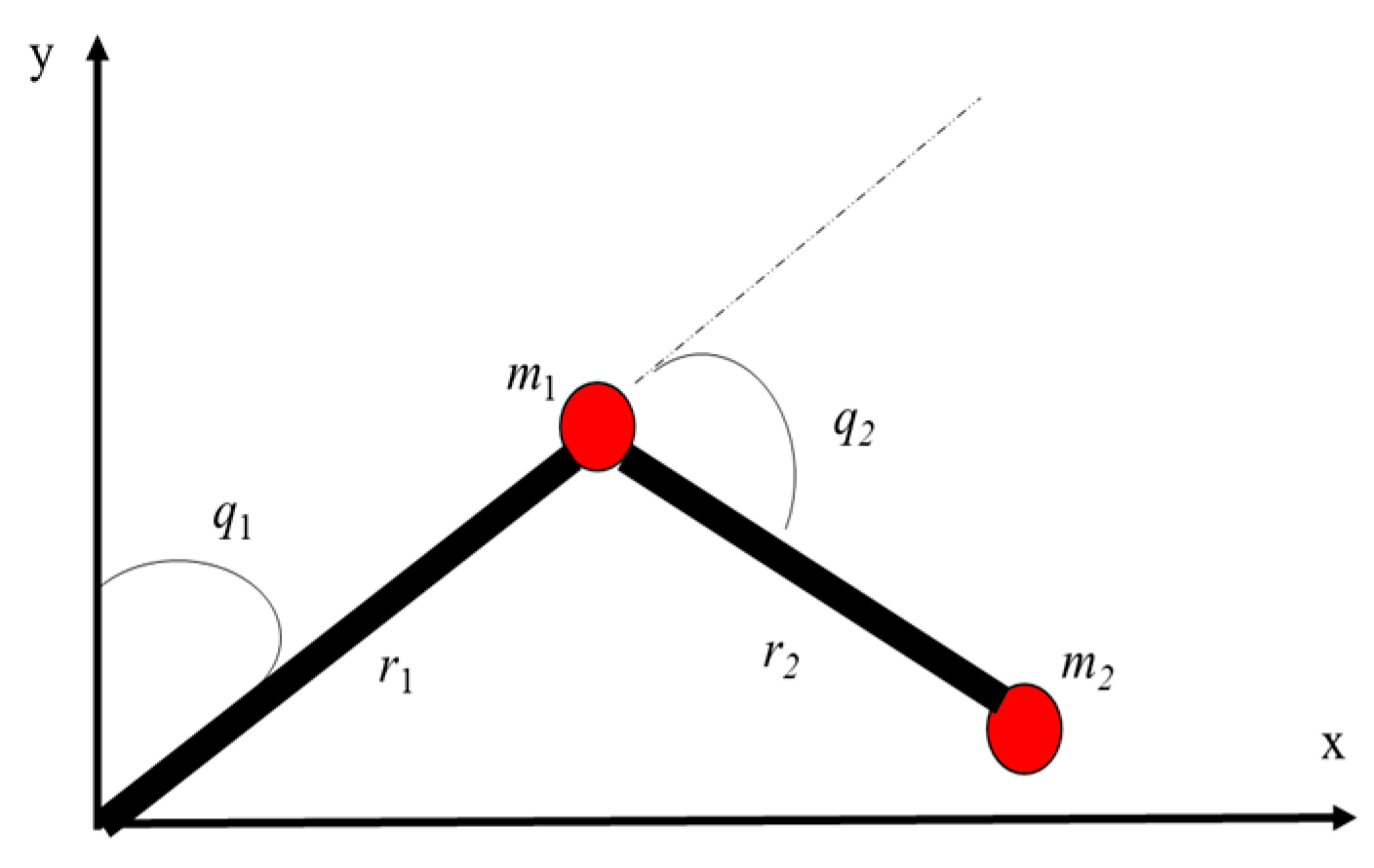
Regarding the significance to potential applications relating to simplicity and robustness, finite-time convergence, and reliable performance under various conditions, the MFTSMC has the capacity to handle uncertainties and nonlinearities to make it a powerful tool in advanced control systems across a broad range of industries. Simulation demonstrations to some critical challenging examples are conducted and compared with model-based approaches for validation, expansion, and applications. Regarding the practical background, the control of a two-link rigid robotic manipulator with two input and two output (TITO) operational mode, a typical multi-degree interconnected nonlinear dynamics tool, is demonstrated to reflect the widely demanded applications in electrical, mechanical, and process industries to reduce labor and improve applicability and reliability in operation.

The rest of the study includes five sections. Section 2 provides the relevant preliminaries. Section 3 designs the MFTSMC system. Section 4 analyzes the MFTSMC attributes in singularity, mitigation of fractional powers in practical implementation, chattering, dynamic inversion, robustness, and the controller tuning rule. Section 5 conducts simulation case studies with three bench test examples. Section 6 summarizes the study and foresees research expansions and applications.

2. Preliminary Information

2.1. Dynamic Plant

Consider a class of general single input single output (SISO) n-th order nonlinear dynamic plant, described by

$${\displaystyle {\sum }_{SISO}: }{y}^{(n)}=f\left(y^{(0\sim n-1)},u,d\right)$$

(1)

where the triplet {$y\in ℝ$, $u\in ℝ$, $d\in ℝ$} represents the plant output, input, and external disturbance, respectively, and $y^{(0\sim n-1)}={\left[y\dots y^{(n-1)}\right]}^T\in {ℝ}^n$ is the $n-1$ order output derivative vector. It should be noted that plant (1) can be expressed in state space equations as well by letting $x=y^{(0\sim n-1)}$ $={\left[\begin{array}{cccc}{x}_1=y& x_2=\dot{y}& \dots & x_n=y^{(n-1)}\end{array}\right]}^T\in {ℝ}^n$ and ${\dot{x}}_n=y^{(n)}=f\left(x,u,d\right)$ [25]. This study treats the plant $f:u\to y$ as a total uncertainty in a black box with enabled control inputs, attainable outputs (either measured or estimated), and a given dynamic order for full state feedback control.

Assumption 1.

The nonlinear system denoted by $\sum (·)$ is stabilizable on a certain specified compact set $D\subseteq {ℝ}^n$ with $\sum (0)=0$, which implies the plant could be non-minimum phase and/or open loop unstable.

Assumption 2.

The plant is completely observable/controllable, where the observability/controllability matrices are non-singular. This makes the designed control system realizable with the feasible signals and control actions.

2.2. Higher-Order TSM Manifold

This study takes the following TSM manifold [4]:

$$\sigma (x)=c_n{x}_n+c_{n-1}\mathrm{sgn}(x_{n-1}){\left|x_{n-1}\right|}^{{\alpha }_{n-1}}+\dots +c_1\mathrm{sgn}(x_1){\left|x_1\right|}^{{\alpha }_1}\in {ℝ}^{n+1}\to ℝ$$

(2)

where $x=y^{(0\sim n)}={\left[\begin{array}{cccc}{x}_1=y& x_2=\dot{y}& \cdots & x_n=y^{(n-1)}\end{array}\right]}^T\in {ℝ}^n$, the coefficient vector $c=\left[\begin{array}{ccc}{c}_n& \cdots & c_1\end{array}\right]\in {ℝ}^n, c_n=1$ is assigned as strictly positive to make the polynomial $x_{n-1}+c_{n-1}{x}_{n-2}\dots +c_1$ Hurwitz stable, and the power parameter vector $\alpha =\left[{\alpha }_{n-1}\cdots {\alpha }_1\right]\in \left.(1-\epsilon ,1)\right|\epsilon \in (0,1)$ is assigned with the following conditions [4]:

$${\alpha }_{i-1}={\displaystyle \frac{{\alpha }_i{\alpha }_{i+1}}{2{\alpha }_{i+1}-{\alpha }_i}},\forall i=2\cdots n-1$$

(3)

where ${\alpha }_n=1$ and ${\alpha }_{n-1}=\lambda ,\hspace{0.33em}\lambda \in (1-\epsilon ,1)$ with $\epsilon \in (0,1)$. Then, for a given $x\ne 0$, the dynamic will asymptotically reach the terminal attractor $x=0$ in finite time $t_s$ while $\sigma =0$.

Consequently, for the second-order TSM manifold below [11], it gives

$$\sigma =\dot{x}+\beta x^{\lambda }$$

(4)

Moreover, the following form of the sliding manifold [4] is introduced in the simulation and implementation

$$\sigma =\dot{x}+\beta {\left|x\right|}^{\lambda }\mathrm{sgn}(x)$$

(5)

where $\beta >0$, $0<\lambda =q/p<1$, $p$ and $q$ are positive odd integers. Then, it has been proved that there exists a finite moment $t_s={\beta }^{-1}{(1-\lambda )}^{-1}{\left|x(0)\right|}^{1-\lambda }$ such that $x(t_s)=0$, which further yields that the terminal attractor $x=0$ is finite time stable, with the tuning parameters $\lambda$ and $\beta$ to regulate the reaching time $t_s$.

2.3. Finite-Time Stability of Homogeneous Systems

Consider a homogeneous system [31] as follows:

$$\dot{y}(t)=f(y(t))$$

(6)

Lemma 1

([31,32]). Suppose there exist an open neighborhood $v$ of the origin, a $C^1$ positive-definite function $V:\nu \to ℝ$ and real numbers $k>0$ and $\alpha \in (0,1)$ such that $\dot{V}+k{V}^{\alpha }$ is negative semi-definite on $v$, where $\dot{V}(y)={\displaystyle \frac{\partial V}{\partial y}}f(y)$. Then, the origin is a finite-time stable equilibrium of (6). Moreover, if $T$ is the settling time function, then it follows that $T(y)\le {\displaystyle \frac{1}{k(1-\alpha )}}V{(y)}^{1-\alpha }$ for all $y$ in some open neighborhood of the origin.

Remark 1.

While the finite-time equilibrium is at the origin, a continuous Lyapunov function exists to satisfy the hypotheses of the above Lemma 1.

Remark 2.

A homogeneous system is finite-time stable iff it is asymptotically stable and has a negative degree of homogeneity. This result considerably simplifies the sufficient Lyapunov conditions involved in differential inequalities [32].

Remark 3.

A finite-time stable homogeneous system has a smooth homogeneous Lyapunov function that satisfies a finite-time differential inequality [31].

3. Model-Free Terminal Sliding Mode Control (MFTSMC)

3.1. Design of MFTSMC Systems

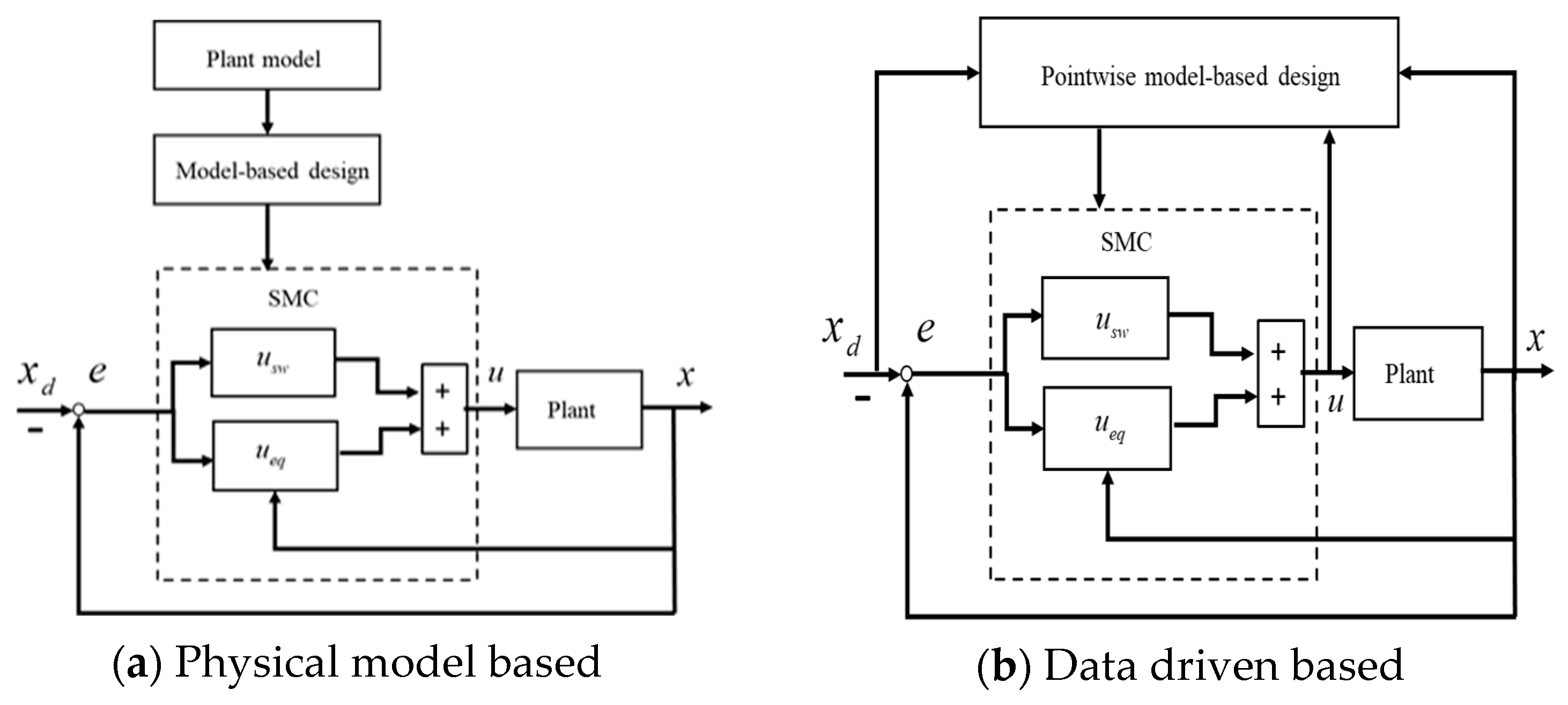
For plant (1), the MFTSMC system is defined as

$${\sum }_{\mathrm{mftsmc}}:\left(\sigma (\tilde{x}),\rho (\tilde{\sigma }),p(*)\right)$$

(7)

where $\sigma (\tilde{x})\in {ℝ}^n\to ℝ$ is the TSM variable, a Hurwitz stable polynomial mapped from the full state error vector $\tilde{x}=x-x_d\in {ℝ}^n$, where $x={\left[\begin{array}{ccc}{x}_1& \cdots & x_n\end{array}\right]}^T\in {ℝ}^n$ and $x_d={\left[\begin{array}{ccc}{x}_{d1}& \cdots & x_{dn}\end{array}\right]}^T\in {ℝ}^n$ are the state vector and the desired state vector to be followed, respectively, and the plant $p(*)$ is defined with (1).

Herein, the control objective is to determine a feedback control $u(\sigma ,\dot{\sigma })=\rho (\sigma )$ to drive the system state $x$ to track a desired trajectory $x_d$ in finite time. To implement the control system, this study proposes a three-step design procedure: (1) assigning the TSM manifold $\sigma (\tilde{x})=\sigma$ in terms of the full state error vector; (2) designing the MF controller $u=\rho (\sigma )$, which is a class of monotonically decreasing functions in the SM coordinate system $(\sigma ,\dot{\sigma })\in {ℝ}^2$ [24]; and (3) configuring the control system. The detailed design process is listed as follows.

(1) Assign the TSM manifold (8) by converting the full state feedback error vector into a finite time stable polynomial, following the formulations defined in Section 2.2:

$$\sigma (\tilde{x})=c_n{\tilde{x}}_n+c_{n-1}\mathrm{sgn}({\tilde{x}}_{n-1}){\left|{\tilde{x}}_{n-1}\right|}^{{\alpha }_{n-1}}+\dots +c_1\mathrm{sgn}({\tilde{x}}_1){\left|{\tilde{x}}_1\right|}^{{\alpha }_1}\in {ℝ}^{n+1}\to ℝ$$

(8)

Specify the parameter vectors $c=\left[\begin{array}{ccc}{c}_n& \cdots & c_1\end{array}\right]\in {ℝ}^n, c_n=1$ and $\alpha =\left[{\alpha }_{n-1}\cdots {\alpha }_1\right]\in \left.(1-\epsilon ,1)\right|\epsilon \in (0,1)$.

(2) Formulate the MF controller by

$$\dot{\sigma }=u={\left.\rho (\sigma )\right|}_{\dot{\sigma }\sigma \le 0}$$

(9)

where $\rho (\sigma )$ denotes certain decreasing monotone functions on the sliding mode plane $(\sigma ,\dot{\sigma })$ satisfying Lyapunov stability conditions $V={\displaystyle \frac{1}{2}}{\sigma }^2>0,V(0)=0$ and $\dot{V}=\dot{\sigma }\sigma <0,\dot{V}(0)=0$.

(3) Configure the control system ${\sum }_{\mathrm{mftsmc}}$.

Figure 3 shows the designed full state feedback control system in a block diagram.

3.2. Model-Free SMC

Theorem 1

(Existence theorem of MFSMC). For designing the MFTSMC system with plant (1) $y^{(n)}=f\left(y^{(0\sim n-1)},u,d\right)$, the following two conditions are held:

(1) The monotonicity, i.e., $\rho (\sigma ):\left\{\begin{array}{c}\rho ({\sigma }_1)>\rho ({\sigma }_2),\forall {\sigma }_1<{\sigma }_2\\ 0,\forall {\sigma }_1={\sigma }_2\end{array}\right.$ is a monotonically decreasing $\mathcal{K}$ function in the sliding mode coordinate system space $(\sigma ,\dot{\sigma })\in {ℝ}^2$.

(2) The boundness, i.e., $|\rho (\sigma )|>|\sup (f)+\alpha (t)|$, where $\sup (f)$ is the bound of the function $f\left(y^{(0\sim n-1)},u,d\right)$ and $\alpha (t)\in ℝ$ is a time varying variable to match $\dot{\sigma }\backslash (y^{(n)},u)=\alpha$.

Then, properly assigned full state feedback sliding mode controller ${\left.u=\dot{\sigma }=\rho (\sigma )\right|}_{\dot{\sigma }\sigma <0,\forall \sigma \ne 0}$ exists to satisfy the control Lyapunov stability condition $V>0|V(0)=0\cap \dot{V}=\dot{\sigma }\sigma <0|V(0)=0$. In addition, for a linear sliding mode manifold, it is a model-free asymptotical control, while it is a model-free finite time control for a terminal sliding mode manifold.

Proof. 

Let $u=\dot{\sigma }=\rho (\sigma )$ in the coordinate system $(\sigma ,\dot{\sigma })$ which is condensed from state space $x\in {ℝ}^n$. For condition (1), $u=\rho (\sigma ), \mathrm{st} \rho (0)=0$ being a strictly decreasing $\mathcal{K}$ function on the $(\sigma ,\dot{\sigma })$ plane, and replace $\dot{\sigma }$ with $u=\dot{\sigma }=\rho (\sigma )$ in the derivative of the Lyapunov function to result in $\dot{V}=\sigma \dot{\sigma }=\dot{\sigma }\sigma =\rho (\sigma )\sigma <0$. This indicates the state vector can converge to its equilibrium. For condition (2), consider $\dot{\sigma }=y^{(n)}+\dot{\sigma }\backslash (y^{(n)},u)+u={\left.f\right|}_{f=y^{(n)}}+\dot{\sigma }\backslash (y^{(n)},u)+\rho (\sigma )$, and let $f+\dot{\sigma }\backslash (y^{(n)},u)+\rho (\sigma )=\sup (f)+\alpha +\rho (\sigma )$. To make $\dot{V}=\dot{\sigma }\sigma <0$, take in the condition $|\rho (\sigma )|>|\sup (f)+\alpha |$. Then, we have $\dot{V}=\dot{\sigma }\sigma =(\sup (f)+\alpha )\sigma +\rho (\sigma )\sigma <0$. For concise expression, let $\sup (f)$ absorb $\alpha$, thus giving $\dot{V}=\dot{\sigma }\sigma =\sup (f)\sigma +\rho (\sigma )\sigma <0$. □

Proposition 1

(Equivalency of model-based and model-free TSMC). Let the model-based controller $u_{mb}\in U_{mb}$ and the model-free controller $u_{mf}\in U_{mf}$, then it follows $U_{mb}\iff U_{mf}$ in terms of sliding mode and Lyapunov stability condition.

Proof. 

Let plant (1) be expressed as ${\displaystyle {\sum }_{SISO}: }{y}^{(n)}=\widehat{f}(y^{(0\sim n-1)})+bu+f_n(*)$, where $\widehat{f}(y^{(0\sim n-1)})+bu$ is a typical nominal output affine model and $f_n\left(*\right)$ denotes the bounded uncertainty and/or disturbance term. From the model-based SMC [22] and Theorem 1, both types of controllers can be formulated in the expressions $u_{mb}={\rho }_1(\dot{\sigma }=0,\widehat{f}(y^{(0\sim n-1)}),b)+{\rho }_2(\sigma ,f_n(*), \mathrm{st} |{\rho }_2(\sigma ,f_n(*)|>\sup (f_n(*)))$ and $u_{mf}=\rho (\sigma ), \mathrm{st}|\rho (\sigma )|>|\sup (f)+\alpha |$, where $\sigma (x)\in {ℝ}^n\to ℝ$ is a general sliding mode manifold of state vector $x\in {ℝ}^n$ and $\rho ,{\rho }_1,{\rho }_2$ are all decreasing $\mathcal{K}$ functions. Therefore, it follows that $U_{mb}\iff U_{mf}$. □

Corollary 1.

Regarding finite time realization of the general sliding mode manifold $\sigma$, consider an integral TSM manifold ${\sigma }_I$ [5] and a convention equivalent TSM manifold [22]. As both approaches are model-based, the equivalencies to the finite time model-free approach are straightforwardly approved.

Corollary 2.

Regarding the robustness with the two types of SMCs, the model-based one has robustness around its nominal model equilibrium point $|{\rho }_2(\sigma ,f_n(*)|>\sup (f_n(*))$ from Corollary 1 and the model-free one has the robustness within the whole domain $|\rho (\sigma )|>|\sup (f)+\alpha |$ from Theorem 1.

Remark 4.

Some of the disadvantages and cautiousness using the model-free control paradigm should be noted and compared with those model-based approaches.

(1) 

Without a model, it is difficult to ANALYZE stability, performance bounds, or robustness formally. Yes, it is true. Regarding DESIGN on the other hand, control Lyapunov functions are in data-driven forms, such as the Lyapunov functions formulated from sliding mode, and then determine the controller output by solving the Lyapunov differential inequality in the MFRUC.

(2) 

Model-free methods are reactive, not predictive. This is an obvious characteristic. This study does not involve predictive control.

(3) 

Model-free controllers may work “well enough” but rarely achieve optimal control (like minimum energy, fastest response, etc.). They often trade off performance for simplicity and robustness. Yes, this MFTSMC cannot provide global optimization, but at most a trial-and-error local optimization.

(4) 

Most data-driven model-free approaches (like reinforcement learning or adaptive controllers) requires an initial learning phase or training phase, which may not be safe or feasible in real-time systems. The MFTSMC does not require such an iterative learning routine.

(5) 

No insight into system dynamics is the common drawback for model-free control. Hopefully, this study provides a possibility to integrate the model-based qualitative knowledge into its control system interpretation and tuning.

(6) 

Tuning controller is empirical, relies on trial and error, heuristics, or data-driven optimization. This can be time-consuming, especially in systems with delays, noise, or nonlinearities. Model-free tuning is even more challenging. This study provides a possibility to integrate the model-based qualitative knowledge into its controller tuning, which is demonstrated in the simulation setups.

Remark 5.

Summarizing the comparisons, the two types of control approaches have supplemented each other in simplicity, robustness, internal dynamic interpretation, optimization, prediction, and so on. MFTSMC has merits in simplicity and robustness in control system design compared to model-based approaches. However, its disadvantages or limitations should be explained as well. The MFTSMC control input could sometimes require relatively large energy spent compared with those model-based approaches; this can be explained by the fact that the model-based approaches determine the control input with reference to the nominal model in its equilibrium neighborhood, and the model-free approach determines the control input by treating the plant as a total uncertainty, which could require large energy in amplitude and/or high frequency to drive the system to the equilibrium from large error states. One more explanation is that the MFTSMC shares similar features of conventional high-gain robust control. Therefore, the stability rendered by this kind of robust control is semi-global, namely, for each upper bound of the uncertainty, there exists a sufficiently high control gain that makes the system stable (e.g., the SMC) to cope with the worst-case scenario [33]. Consequently, in application, the actuator operation limits should be carefully checked to avoid saturation while considering the MFTSMC.

Proposition 2

(Expansion to interconnected MIMO control systems). It is noted that this type of dynamically interconnected plant has no input–output coupling, and accordingly, the MIMO plants can be treated as m SISO systems, which further gives the following result.

Referring to plant (1), the MIMO plant can be expressed as ${\displaystyle {\sum }_{MIMO}: }{y}_i^{(n)}=f_i\left(Y^{(0\sim n-1)},u_i,d_i\right),i=1\cdots m$, where $Y^{(0\sim n-1)}={\left[\begin{array}{ccc}{y}_1^{(0\sim n-1)}& \cdots & y_m^{(0\sim n-1)}\end{array}\right]}^T$, then the corresponding SMs and controllers are formulated as the diagonal elements in the form of $\sigma =\mathrm{diag}\left\{\begin{array}{ccc}{\sigma }_1& \cdots & {\sigma }_m\end{array}\right\}$ and $u=\mathrm{diag}\left\{\begin{array}{ccc}{u}_1& \cdots & u_m\end{array}\right\}=\mathrm{diag}\left\{\begin{array}{ccc}{\mathrm{tsmc}}_1& \cdots & {\mathrm{tsmc}}_m\end{array}\right\}$ [34]. QED.

Remark 6.

For those fully actuated MIMO coupling plants, a new study is required. It is noted that model-free asymptotic SMC for this class of plants has been developed for robust decoupling control of nonlinear nonaffine dynamic systems [35]; this could provide a foundation to expand it into the MIMO MFTSMC in the following studies. For underactuated MIMO plants, developing such an MFTSMC is more challenging. Comparing the control of SISO and MIMO systems, the first critical difference is the input–output coupling effect, and the second is the underactuated mode.

Corollary 3.

Rather than just limited solutions from equality ${\left.u=\rho (\sigma )\right|}_{\dot{\sigma }=0}$ with model-based SMC, there are various options for selecting the MFSMC controller ${\left.u=\rho (\sigma )\right|}_{\dot{\sigma }\sigma <0}$, which provides infinite solutions for this type of controller. In the following, this study provides two types of controllers, with both switching control $u_{sw}$ and equivalent control $u_{eq}$, and continuous (non-switching) control satisfying the condition of $\rho (\sigma )\sigma <0$ [25].

(1) 

Proportional and Integral (PI) function

A PI-function for the controller design can be formulated by

$$u=\dot{\sigma }=u_{eq}+u_{sw}={\left.(-k_p\sigma -k_i{\displaystyle \int \sigma })\right|}_{\left|\sigma \right|\le \delta }-k_g{\left.\mathrm{sgn}(\sigma )\right|}_{\left|\sigma \right|>\delta }$$

(10)

where $u_{sw}$ denotes the switching control law and $u_{eq}$ represents the equivalent control term, the associated constant gains satisfy $k_p,k_g>\left|\sup (f)+\alpha \right|,k_i>0$ $k_p\gg k_i, \left|\left(k_p\right){\sigma }^2\right|>\left|\left(k_i\right)\sigma {\displaystyle \int \sigma d\tau }\right|$, and $\delta$ is the sliding mode boundary distance function (also known as the boundary thickness in the study) to the sliding mode $\sigma (x)=0$ with $L^2$ norm, i.e., $\delta ={‖\sigma (x)-\sigma (0)‖}_2$. In the position, for $\forall \sigma \ne 0$, the corresponding control Lyapunov function $V$ requires the following conditions:

$$\begin{array}{l}V={\sigma }^2>0\\ \dot{V}=\dot{\sigma }\sigma =\left\{\begin{array}{ccc}\left(-k_g\mathrm{sgn}(\sigma )\sigma \right)<0,& k_g>\left|\sup (f)\right|& \forall u_{sw}\\ -k_p{\sigma }^2-k_i\sigma {\displaystyle \int \sigma }<0,& \left\{\begin{array}{c}{k}_p>\left|\sup (f)\right|\\ \left|k_p{\sigma }^2\right|>\left|k_i\sigma {\displaystyle \int \sigma }\right|\end{array}\right.& \forall u_{eq}\end{array}\right.\end{array}$$

(11)

Otherwise, $V=\dot{V}=0,\forall \sigma =0$.

(2) 

Continuous (non-switching) SMC

Consider a monotone bounded sigmoid function to replace the switching SMC below

$$\dot{\sigma }=u=-k_{h}sigmoid(k_0\sigma )+{\displaystyle \frac{k_h}{2}}$$

(12)

where $k_h>\left|\sup (f)\right|$ and $k_0>0$. Then, for $\forall \sigma \ne 0$, the Lyapunov stability conditions are satisfied below:

$$\begin{array}{c}V={\sigma }^2>0\\ \dot{V}=\dot{\sigma }\sigma =(-k_{h}sigmoid(k_0\sigma )+{\displaystyle \frac{k_h}{2}})\sigma <0\end{array}$$

(13)

Otherwise, $V=\dot{V}=0,\forall \sigma =0$.

Herein, the constant gains $k_h>0$ and $k_0>0$ jointly regulate the controller amplitude and convergent speed. Accordingly, the non-switching (continuous) SMC output is formulated as a special case of the switching SMC in the form of $\dot{\sigma }=u=\rho (\sigma )=\begin{array}{cc}-k_{h}sigmoid(k_0\sigma )+{\displaystyle \frac{k_h}{2}},& \forall u_{eq}\end{array}=u_{sw}\in u$.

Remark 7.

The TSMC, satisfying the Lyapunov differential inequality $\dot{V}+k{V}^{\alpha }\le 0$, is stably equivalent to the inequality $\dot{V}+kV\le 0$ with linear asymptotic SMC (LASMC). However, the difference is the finite time terminal sliding mode against the asymptotic time sliding mode in convergency, which can be explained by considering $\dot{V}+k{V}^{\alpha }=\dot{V}+k{({\sigma }^2)}^{\alpha }=\dot{V}+k{({\sigma }^{\alpha })}^2\sim \dot{V}+kV$.

4. Property Analysis

4.1. Singularity Analysis

Take an example to explain the cause of the singularity. Consider a second-order dynamic described in (1) as $\ddot{y}=f\left(y,\dot{y},d\right)+bu, b\ne 0$. Further, to express it as the state space model realization, let $x={\left[\begin{array}{cc}{x}_1=y& x_2=\dot{y}\end{array}\right]}^T\in {ℝ}^2$, then it gives $\left\{\begin{array}{l}{\dot{x}}_1=x_2\\ {\dot{x}}_2=f\left(x,d\right)+bu\end{array}\right.$. Moreover, set up the TSM manifold as $\sigma =x_2+\beta x_1^{\lambda }, 0<\lambda <1$. Accordingly, its derivative is derived as $\dot{\sigma }={\dot{x}}_2+\beta \lambda {\dot{x}}_1{x}_1^{\lambda -1}={\dot{x}}_2+\beta \lambda x_2{x}_1^{\lambda -1}$. Consequently, the singularity appears in ${\left.x_1^{\lambda -1}\right|}_{0<\lambda <1}\to \infty ,\forall x_1\to 0$.

Lemma 2

(inherent singularity in model-based SMC). The singularity is the inheritance with the model-based TSMC, where the TSMC must possibly be infinitely large to keep the desired TSM motion. This problem is actually induced by a series of mappings from the TSM manifold to the TSMC output $u$ as $\sigma (*,x^{\lambda })\to \dot{\sigma }(*,x^{\lambda -1})\to {\left.u(*,x^{\lambda -1})\right|}_{\dot{\sigma }=0}$; thus, it follows $x\to 0$, ${\left.x^{\lambda -1}\right|}_{0<\lambda <1}\to \infty$, and $u(\dot{\sigma })\to \infty$.

Regarding model-based TSMC design, still using the second-order dynamic example, let the derivative of an SM manifold $\dot{\sigma }={\dot{x}}_2+\beta \lambda {\dot{x}}_1{x}_1^{\lambda -1}={\dot{x}}_2+\beta \lambda x_2{x}_1^{\lambda -1}=0$, which can be expressed explicitly with the control output $u$ with reference to the plant, then it gives $\dot{\sigma }={\dot{x}}_2+\beta \lambda x_2{x}_1^{\lambda -1}=f\left(x,d\right)+bu+\beta \lambda x_2{x}_1^{\lambda -1}=0$; consequently, the TSMC is designed with $u=-\left(\widehat{f}\left(x\right)+\beta \lambda x_2{x}_1^{\lambda -1}\right)/b-k\mathrm{sgn}(\sigma )$, where $\widehat{f}\left(x\right)$ is the nominal model of $f\left(x,d\right)$. Note that there are several zones for the pair $x_2{x}_1^{\lambda -1}$ around origin $(0,0)$ to induce the singularity ${\left.x_2{x}_1^{\lambda -1}\right|}_{x_1=0\cap x_2\ne 0}\to \infty$ as the negative power term $x_1^{\lambda -1},\forall 0<\lambda <1$ in the phase plane [11].

Even though various approaches have been derived to remove the singularity, the problem inherently exists in the model-based TSMC if the derivative of the sliding mode is used for the solution of the controller output $u$.

Lemma 3

(global nonsingularity in model-based SMC). The singularity does not exist in the model-free TSMC, because the MFTSMC design follows the routine $\sigma (*,x^{\lambda })\to \rho (\sigma )\to {\left.u(*,\sigma )\right|}_{\dot{\sigma }\sigma <0}$, while $x\to 0$, ${\left.x^{\lambda }\right|}_{\lambda <1}\to 0$. Therefore, this is a globally nonsingular TSM, as there is no negative fractional power throughout the formulation.

Regarding model-free TSMC design, take the same TSM manifold and the Lyapunov function to determine the control $u$ by the criterion $\dot{\sigma }\sigma <0$ rather than using $\dot{\sigma }=0$ (the model-based design). From the existence theorem, assign $u=-k_p\sigma -k\mathrm{sgn}(\sigma )=-k_p(x_2+\beta x_1^{\lambda })-k\mathrm{sgn}(\sigma )$, where $k_p>\sup \left|f\left(x,d\right)\right|$. Obviously, there is no term of $x_1^{\lambda -1}$ to induce the singularity problem in the control. Therefore, the model-free TSMC is globally nonsingular.

4.2. Mitigation of Fractional Powers—Practical Implementation

While the controller is designed to ensure nonsingular behavior theoretically, the presence of fractional powers in some sliding surfaces could pose practical challenges, particularly in the presence of sensor noise or data quantization. To address this concern, the following mitigation strategies could be useful in applications:

(1)

Smoothing approximations: Replace the fractional power terms with smooth, bounded approximations (e.g., using a saturation or sigmoid function) in a boundary layer near the origin to prevent singularities or excessive sensitivity to noise [36].

(2)

Signal filtering: Apply low-pass filtering to the measured signals before computing the fractional power terms to reduce the impact of high-frequency noise. Care is taken to minimize phase lag and avoid destabilizing the feedback loop [37].

(3)

Discretization handling: In digital implementations, the fractional exponents can be regularized near zero to avoid numerical instability (e.g., replacing $\left|x^{1/3}\right|$ with ${(|x|+\epsilon )}^{1/3},\epsilon >0$ [37]).

(4)

Alternative sliding surfaces: If needed, equivalent sliding surfaces using higher-order error dynamics (e.g., super-twisting-type surfaces or robust integral terms) can be considered, which maintain robustness without relying on fractional powers [38].

4.3. Chattering Suppression

Proposition 3.

Chattering potentially exists in a closed loop dynamic system with (1) unmodelled fast dynamics (with small time constants) neglected in nominal model [18]; (2) switching hard nonlinear element(s), where the elements could be on-ff, saturation, dead-zone, backlash and hysteresis functions [2]; (3) continuous nonlinearities such as power fractional variable used in TSM manifolds [19]; (4) it should be mentioned that finite sampling rate in digital controllers could induce chattering as well [18]. For the continued time control in this study, we will not address the discrete time effect in analyzing the chattering effects.

The MFTSMC involves power-fractional SM (PFSM), a signinum function from switching control to equivalent control, and nonlinear dynamic plant (with known dynamic order). The measures to avoid chattering with the MFTSMC include:

(1)

Dealing with stable oscillation by removing negative semi-definite stability condition $\dot{\sigma }=0$ with negative definite stability $\dot{\sigma }\sigma <0$ in the controller design, and consequently, removing the constant oscillation in the neighbourhood of the origin.

(2)

Dealing with switching hard nonlinearity by increasing the sliding mode manifold boundary layer thickness $\delta$. To reduce the hard nonlinearity, induce a chattering opportunity in the vicinity of the convergent point (normally $x=0$). It is noted that properly enlarged thickness $\delta$ does not reduce accuracy, as once on the sliding mode boundary, the error vector converges towards the origin in finite time. The combination of the switching control and equivalent control forms a control law with saturation function [39].

(3)

Dealing with fractional power nonlinearity by reducing the relative degree of the systems. Let m be the extra order of the unmodeled dynamics from a given nth order dynamic plant. Thus, a limit cycle/periodic motion may occur in the system with power-fractional SM (PFSM) while the total relative degree of the actuator, plant and sliding surface is above two, because the Nyquist plot of the linear part intersects the negative part of the real axis in this case [19]. To cope with this problem, the proposed approach adopts a mode-free extended state observer ([24,40]) with dynamic order n + m and accordingly increases the dynamic order of the sliding mode manifold to n + m − 1, so that the resultant relative degree is (n + m) − (n + m − 1) = 1.

(4)

Avoiding high gain control, in general, the MFTSMC has a relatively large range of gains for achieving almost the same operational performance at the system outputs. Try to use low gain while keeping the similar output performance, and consequently, avoid the limit cycle induced by high gain in the nonlinear dynamic systems.

4.4. Nonlinear Dynamic Inversion (NDI) Though MFTSMC

It is noted that some work has been linked to model-based linear SM-based NDI [41] and model-free linear SMC-based NDI as well [24,25], which is a dynamic stabilization process. Similarly, the MFTSMC shares the ability to achieve NDI, but achieves it in finite time.

Theorem 2

(NDI). If there exists a control $\dot{\sigma }=u=\rho (\sigma )$ satisfying the Lyapunov differential inequality $\dot{V}=\dot{\sigma }\sigma <0$ in the MFTSMC, to achieve $\sigma (x(t))=0\to x(t)-x_d(t)=0,\to x(t)=I_n{x}_d(t),$ $\forall t\ge t_s$, then the dynamic inversion in the MFTSMC closed loop gives $C_{NDI}({\widehat{P}}^{-1},P)=I_n,\forall t\ge t_s$.

Proof. 

For easy proof, let (1) a single input and single output (SISO) plant, as expressed in (1), $P:y^{(n)}=f\left(y^{(0\sim n-1)},u,d\right)$; (2) the full state feedback terminal sliding mode be $\sigma (\tilde{x})={\tilde{x}}_n+c_{n-1}\mathrm{sgn}({\tilde{x}}_{n-1}){\left|{\tilde{x}}_{n-1}\right|}^{{\alpha }_{n-1}}+\dots +c_1\mathrm{sgn}({\tilde{x}}_1){\left|{\tilde{x}}_1\right|}^{{\alpha }_1}$, where $\tilde{x}={\left[\begin{array}{ccc}{x}_n-x_d^{(n-1)}& \dots & x_1-x_d\end{array}\right]}^T$ is the error vector between the state vector $x$ and the desired state vector $x_d$; (3) the controller ${\widehat{P}}^{-1}=tsmc$, functioned as $u=\left\{\begin{array}{cc}{u}_{sw}=-k_g\mathrm{sgn}(\sigma )& \forall \left|\sigma \right|>\delta \\ u_{eq}=\rho (\sigma )& \forall \left|\sigma \right|\le \delta \end{array}\right.$; and (4) the corresponding closed loop control system be $C_{NDI}({\widehat{P}}^{-1},P)$. From Theorem 1, there exist such asymptotic terminal controllers to obtain $C_{NDI}({\widehat{P}}^{-1},P): \sigma (\tilde{x}(t))=0,\forall \tilde{x}(t)=0, \forall t\ge t_s$, which means $\tilde{x}(t)=x(t)-x_d(t)=0, \forall t\ge t_s$, that is, $x(t\ge t_s)=I_n{x}_d(t\ge t_s)$ to prove the relationship from the input $x_d$ to the output $x$ through the closed loop control system ${\left.C_{NDI}({\widehat{P}}^{-1},P)\right|}_{t\ge t_s}=I_n$. □

4.5. Robustness Analysis [42]

For a general dynamic system $y^{(n)}=f\left(y^{(0\sim n-1)},u,d\right)$ as expressed in (1), the robustness is characterized by means of the sensitivity of the closed-loop model, specifically, the transfer function in linear cases, to variations in plant parameters. Let $T(f)$ be an expression of the control system performance linked with one or more plant parameters [43]; a general model-based system sensitivity function expanded from linear transfer function is defined as the ratio of the percentage change in the closed-loop performance to the percentage change in the plant [44]:

$$S_f^T={\displaystyle \frac{\partial T(f)/T}{\partial f/f}}={\displaystyle \frac{\partial T(f)}{\partial f}}{\displaystyle \frac{f}{T}}$$

(14)

When the plant is considered entirely uncertain, it becomes challenging to perform the above analysis without an explicit analytical model. As an alternative, the system’s sensitivity function can be symbolically defined in a model-free manner as:

$$S_f^T={\displaystyle \frac{\Delta T(f)}{\Delta f}}{\displaystyle \frac{f}{T}}$$

(15)

The sensitivity function reduction means the robustness will be enhanced in dynamic control systems [43].

Remark 8.

For a stabilizable plant ${\displaystyle {\sum }_{SISO}: }{y}^{(n)}=f\left(y^{(0\sim n-1)},u,d\right)$ ${\left|f\right|}_{\max }\le F=\sup (\left|f\right|)\in {ℝ}^{+}$, from Theorem 1, there exists a control ${\left.u=\rho (\sigma )\right|}_{\dot{\sigma }\sigma <0}$ to stabilize the control system while keeping the dynamic performance within the invariant TSM. From Theorem 2, the inversion of the nonlinear dynamics, the closed loop performance is characterized by ${\left.T\right|}_{t\ge t_s}=I_n$, that is, the variation ${\left.\Delta T=0\right|}_{\Delta f\ne 0}$, where $\Delta T\in S\subset {ℝ}^n$ with $S$ a compact set. Consequently, the system sensitivity for the model-free control systems is determined by $S_f^T={\displaystyle \frac{\Delta T(f)}{\Delta f}}{\displaystyle \frac{f}{T}}={\left.{\displaystyle \frac{0}{\Delta f}}{\displaystyle \frac{f}{T}}\right|}_{\Delta f\ne 0}=0, \forall \Delta T\in S\subset {ℝ}^n$, which is considered as a form of total robustness within the bound $S$. For model-based control systems, as ${\left.\Delta T\ne 0\right|}_{\Delta f\ne 0}$, it gives $S_f^T={\displaystyle \frac{\Delta T(f)}{\Delta f}}{\left.{\displaystyle \frac{f}{T}}\right|}_{\Delta f\ne 0}\ne 0$, which is proportional robustness control against the system uncertainty.

4.6. Controller Parameter Tuning

Once the TMS assigned [4], the rest of the work is to tune the assigned controller parameters, in which each of the controllers PI ($k_g,k_p,k_i$) and sigmoid function ($k_h,k_0$) has two or three parameters selected. The controller parameter (gains) tuning is guided with Theorem 1: Once a controller $u=\rho (\sigma )$ is selected, the rest of the work is to tune the gains in the controller for simulations and applications. As the plant up bound $\sup (f)$ is unknown, we take a trial-and-error iterative approach to tune the controller parameters (gains) in a systematic routine. Let $u=\rho (\sigma )=-K{\rho }_1(\sigma ), K\in ℝ$, starting a trial value of $K$ with experience, which could have two types of responses, stable or instable. The rule is that large gain increases the stability to improve the control effect. Once the desired response is achieved, gradually reduce the gain until a value keeping the desired response, which reduces the energy cost and avoids controller output saturation in applications. For PI-type controllers, the integral gain is set at a reasonable small value, sometimes not necessarily added. Another added value in the tuning is that the TSMC cooperates with P, PI controllers (D control has been absorbed in the derivative of the sliding mode [25]), and the gains can be more straightforwardly tuned. The comparisons between the three types of PIDs, conventional output error PID, PID sliding mode, and full state error sliding mode PID, can be found in a recent publication [25]. For tuning the sigmoid controller, the constant gains $k_h>0$ and $k_0>0$ jointly regulate the controller amplitude and convergent speed under the condition of $k_h>\left|\sup (f)\right|$ and $k_0>0$.

It should be noted that the controller parameters are selectable within a large domain specified by the Lyapunov differential inequality, rather than those model-based controls selecting controller parameters within their neighborhood of Lyapunov differential equality. Consequently, the controller parameter tuning is robust in relatively large domains for the simulation and application setups.

5. Case Studies

Three case studies are selected for demonstrating the proposed MFTSMC in functional configuration and numerical/computational experiments, also showing off the step-by-step design/test application procedure for potential expansions. It should be mentioned that the plant models used in the case studies are only used for simulating the dynamic plant operation, with nothing referring to the controller design due to the nature of designing the total model-free control. The major objectives include:

(1)

selecting three bench tests on nonlinear dynamic plants from the representative numerical models to the real physical plant model;

(2)

designing the MFTSMC system to accommodate the performance in robust stability, transient/steady state response, removing singularity, supressing chattering effects;

(3)

developing the simulation platform with MATLAB (R2024a)/Simulink and running the simulation tests with robust parameter tuning;

(4)

analyzing the MFTSMC performance, as reflected in the generated simulation plots;

(5)

comparing the MFTSMC with a delegate work in model-based higher-order nonsingular TMSC [5], and a complex third-order non-affine nonlinear plant, and a representative model-based TSMC for two-link rigid robotic manipulator [22].

5.1. Bench Test Plants

Plant 1: Consider a third-order output affine nonlinear plant described below, which has been used as bench test of model-based TMSC [5]:

$$P\left(y^{(3)}=f\left(y^{(0\sim 2)},u,d\right)\right): y^{(3)}=y^2\dot{y}+{\ddot{y}}^2+100u+d$$

(16)

where triplet $\left\{\begin{array}{ccc}y& u& d\end{array}\right\}$ represents the plant output, input, and the external disturbance, respectively.

The polynomial plant can be expressed in the state space model, by assigning $x=y^{(0\sim 2)}$ $={\left[\begin{array}{ccc}{x}_1=y& x_2=\dot{y}& x_3=\ddot{y}\end{array}\right]}^T$, as

$$\begin{array}{c}{\dot{x}}_1=x_2\\ {\dot{x}}_2=x_3\\ {\dot{x}}_3=x_1^2{x}_2+x_3^3+100u+d\end{array}$$

(17)

The initial state vector is set as ${\left[\begin{array}{ccc}{x}_1(0)& x_2(0)& x_3(0)\end{array}\right]}^T={\left[\begin{array}{ccc}1& 1& 1\end{array}\right]}^T$. The external disturbance is assigned as $d(t)=100+30\sin (2\pi t)$, and is assumed to add on the system from the time instant $t=15$. This plant is globally unstable to the initial state with the simulation test.

Plant 2: Consider a third-order non-affine nonlinear plant described below, in which the second-order polynomial has been bench-tested with model-free linear SMC [25]:

$$P\left(y^{(3)}=f\left(y^{(0\sim 2)},u,d\right)\right): y^{(3)}=-{\ddot{y}}^3-y\dot{y}-u\dot{y}-0.6y+\sin (u)+2u+u^3+d$$

(18)

To facilitate full state feedback control, express the polynomial plant in the state space model, by assigning $x=y^{(0\sim 2)}={\left[\begin{array}{ccc}{x}_1=y& x_2=\dot{y}& x_3=\ddot{y}\end{array}\right]}^T$, as

$$\begin{array}{c}{\dot{x}}_1=x_2\\ {\dot{x}}_2=x_3\\ {\dot{x}}_3=-x_3^3-x_1{x}_2-u{x}_2-0.6x_1+\sin (u)+2u+u^3+d\end{array}$$

(19)

The initial state vector is set as ${\left[\begin{array}{ccc}{x}_1(0)& x_2(0)& x_3(0)\end{array}\right]}^T={\left[\begin{array}{ccc}1& 1& 1\end{array}\right]}^T$. The external disturbance is the same as used in the first plant test. This plant is locally stable to the initial state with the simulation test, which for a positive step input, it has $\left|x(\infty )\right|<\infty ,\forall u(t)=c\in {ℝ}^{+}$.

Plant 3: As shown in Figure 4, this two-link rigid robotic manipulator is an example of two input and two output (TITO) operational mode. This is a typical multi-degree interconnected nonlinear dynamics tool that has been widely used in electrical, mechanical, and process industries to reduce labor and improve accuracy in operation [36,45]. The manipulator’s Euler–Lagrange motion equation is expressed as below [22].

$$M(q)\ddot{q}+C(q,\dot{q})\dot{q}+G(q)=\tau +{\tau }_d$$

(20)

where $q=col(q_1,q_2)\in {ℝ}^2$ is the joint angular position, $M(q)=\left[\begin{array}{cc}{m}_{11}(q)& m_{12}(q)\\ m_{21}(q)& m_{22}(q)\end{array}\right]\in {ℝ}^{2\times 2}$ denotes the positive definite inertia matrix, $C(q,\dot{q})={\left[\begin{array}{cc}{c}_1(q,\dot{q})& c_2(q,\dot{q})\end{array}\right]}^T\in {ℝ}^2$ is the vector of centripetal and Coriolis torque vector, $G(q)={\left[\begin{array}{cc}{g}_1(q)& g_2(q)\end{array}\right]}^T\in {ℝ}^2$ is the gravitational torque vector, $\tau =col({\tau }_1,{\tau }_2)\in {ℝ}^2$ is the supplied torque/force vector as the control input to drive the manipulator, and ${\tau }_d={[\begin{array}{cc}{\tau }_{d1}& {\tau }_{d2}\end{array}]}^T\in {ℝ}^2$ is the vector representing the bounded lumped external disturbances.

For the simulation demonstrations, the manipulator parameters [22] are specified with the plant of $r_1$ = 1 m, $r_2$ = 0.8 m, $J_1$ = 5 kg m², $J_2$ = 5 kg m², $m_1$ = 0.5 kg, $m_2$ = 1.5 kg, $g$ = 9.8 m/s². The trajectory references are set up by $q_{ref1}=1.25-(7/5)e^{-t}+(7/20)e^{-4t}$ and $q_{ref2}=1.25+e^{-t}-(1/4)e^{-4t}$. The system states are initialized with $q_1(0)=1.0, {\dot{q}}_1(0)=0$; $q_2(0)=1.5$,${\dot{q}}_2(0)=0$. The system external disturbances are assumed to be time varying sequences with ${\tau }_{d1}=2\sin (t)+0.5\sin (200\pi t)$ and ${\tau }_{d2}=\cos (2t)+0.5\sin (200\pi t)$, in which the second element represents high-frequency measurement noise. The corresponding elements in the matrix and vectors are shown below.

For the inertia matrix $M(q)$:

$$\begin{array}{l}{m}_{11}(q_2)=(m_1+m_2)r_1^2+m_2{r}_2^2+2m_2{r}_1{r}_{2}cos(q_2)+J_1\\ m_{12}(q_2)=m_{21}(q_2)=m_2{r}_2^2+m_2{r}_1{r}_{2}cos(q_2)\\ m_{22}=m_2{r}_2^2+J_2\end{array}$$

For the centripetal and Coriolis torque $C(q,\dot{q})\dot{q}$:

$$\begin{array}{l}{c}_1(q,\dot{q})\dot{q}=-b_{12}(q_2){\dot{q}}_1^2-2b_{12}(q_2){\dot{q}}_1{\dot{q}}_2\\ c_2(q,\dot{q})\dot{q}=b_{12}(q_2){\dot{q}}_2^2\\ b_{12}(q_2)=m_2{r}_1{r}_2\sin (q_2)\end{array}$$

For the is the gravitational torque:

$$\begin{array}{l}{g}_1(q)=\left((m_1+m_2)r_{1}cos(q_2)+m_2{r}_{2}cos(q_1+q_2)\right)g\\ g_2(q)=\left(m_2{r}_{2}cos(q_1+q_2)\right)g\end{array}$$

5.2. Selection of the Controllers and Parameters

The first two MFTSMC systems are designed with the same TSM manifold, and proportional + integral (PI) controllers, in which the parameters ($k_g,k_p,k_i,\delta$) are tuned in simulation and are listed in

Table 1. MFTSMC with plant 1.

TSM (8) $\sigma ={\tilde{x}}_3+c_2\mathrm{sgn}({\tilde{x}}_2){\left|{\tilde{x}}_2\right|}^{{\alpha }_2}+c_1\mathrm{sgn}({\tilde{x}}_1){\left|{\tilde{x}}_1\right|}^{{\alpha }_1}$	Parameters $\begin{array}{cc}{c}_1=4& c_2=4.2\\ {\alpha }_1=1/3& {\alpha }_2=1/2\end{array}$
Controller (10) $u=\dot{\sigma }=\left\{\begin{array}{cc}{u}_{sw}=-k_g\mathrm{sgn}(\sigma )& \forall \left|\sigma \right|>\delta \\ u_{eq}=\rho (\sigma )=-k_p\sigma -k_i{\displaystyle \underset{0}{\overset{t}{\int }}\sigma d\tau }& \forall \left|\sigma \right|\le \delta \end{array}\right.$	Parameters $\begin{array}{lll}{k}_g=10& \begin{array}{cc}{k}_p=10& k_i=0.8\end{array}& \delta =1\end{array}$

and

Table 2. MFTSMC with plant 2.

TSM (8) $\sigma ={\tilde{x}}_3+c_2\mathrm{sgn}({\tilde{x}}_2){\left|{\tilde{x}}_2\right|}^{{\alpha }_2}+c_1\mathrm{sgn}({\tilde{x}}_1){\left|{\tilde{x}}_1\right|}^{{\alpha }_1}$	Parameters $\begin{array}{cc}{c}_1=4& c_2=4.2\\ {\alpha }_1=1/3& {\alpha }_2=1/2\end{array}$
Controller (10) $u=\dot{\sigma }=\left\{\begin{array}{cc}{u}_{sw}=-k_g\mathrm{sgn}(\sigma )& \forall \left|\sigma \right|>\delta \\ u_{eq}=\rho (\sigma )=-k_p\sigma -k_i{\displaystyle \underset{0}{\overset{t}{\int }}\sigma d\tau }& \forall \left|\sigma \right|\le \delta \end{array}\right.$	The parameters $\begin{array}{lll}{k}_g=100& \begin{array}{cc}{k}_p=100& k_i=15\end{array}& \delta =1\end{array}0$

, respectively.

For the third TITO MFTSMC system,

Table 3. MFTSMC with plant 3.

TMC (8) $\sigma =diag({\sigma }_1,{\sigma }_2)$ $\begin{array}{l}{\sigma }_1={\dot{\tilde{q}}}_1+c_1\mathrm{sgn}({\tilde{q}}_1){\left|{\tilde{q}}_1\right|}^{{\alpha }_1}\\ {\sigma }_2={\dot{\tilde{q}}}_2+c_2\mathrm{sgn}({\tilde{q}}_2){\left|{\tilde{q}}_2\right|}^{{\alpha }_1}\end{array}$	Parameters $c=diag(c_1,c_2)$ $\begin{array}{cc}{c}_1=1& {\alpha }_1=2/3\\ c_2=1& {\alpha }_2=2/3\end{array}$
Controller (11) $\begin{array}{l}{\dot{\sigma }}_i={\tau }_i={\rho }_i({\sigma }_i)=-k_{hi}\tanh (k_{0i}{\sigma }_i)\\ i=1,2\end{array}$	Parameters $\begin{array}{cc}{k}_{h1}=100& k_{01}=80\\ k_{h2}=100& k_{02}=80\end{array}$

shows TSM and the continuous controller parameters.

Controller parameter tuning provides guidance for tuning the above controller parameters for the simulation demonstrations. A procedure has been carried out for trial-and-error optimal searching of the controller parameters. The key steps are outlined below.

(1)

Define the control objectives: stabilization, state response, control input, etc.

(2)

Identify the control parameters, as specified with two or three parameters for each controller.

(3)

Set up constraints for all the controller parameters’ positive and proposal gains larger than estimated uncertainty bounds.

(4)

Start with an initial guess or reasonable solution to test the knowledge and experience of the control systems.

(5)

Test the different solutions, as explained in Section 4.5 <Controller parameter tuning>.

(6)

Iterate the test procedure to narrow the range or adjust around the promising solutions.

(7)

Choose the solution that best meets the control objectives while satisfying all the constraints.

5.3. Discussions on the Simulated System Performance

In the Simulink (MATALB R2024a) simulation, the three plants are treated as unknown dynamic gains in black boxes with measurable states and enable control inputs externally, which are typical problems in control of total uncertainty systems [39,42].

Plant 1: Figure 5 shows the test of the system against external disturbances. These simulated sequences are like those obtained from the representative model-based TSMC [5]. This demonstrates the equivalency of model-based and model-free TSMC in terms of sliding mode and Lyapunov stability condition. There are several aspects to be explained for the generated plots.

(1)

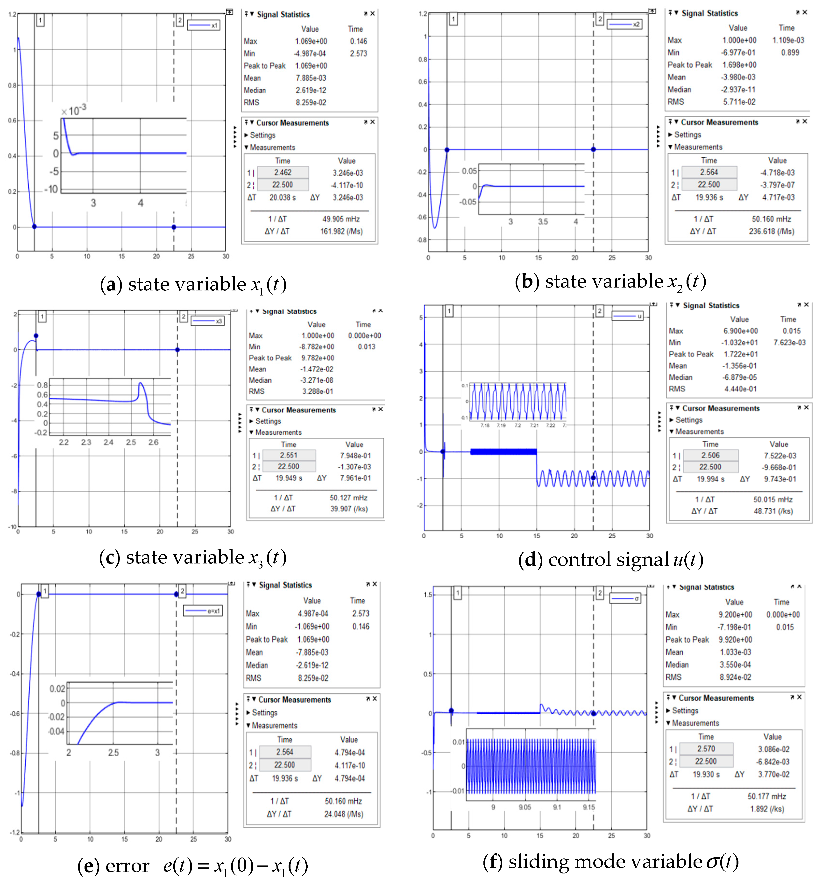
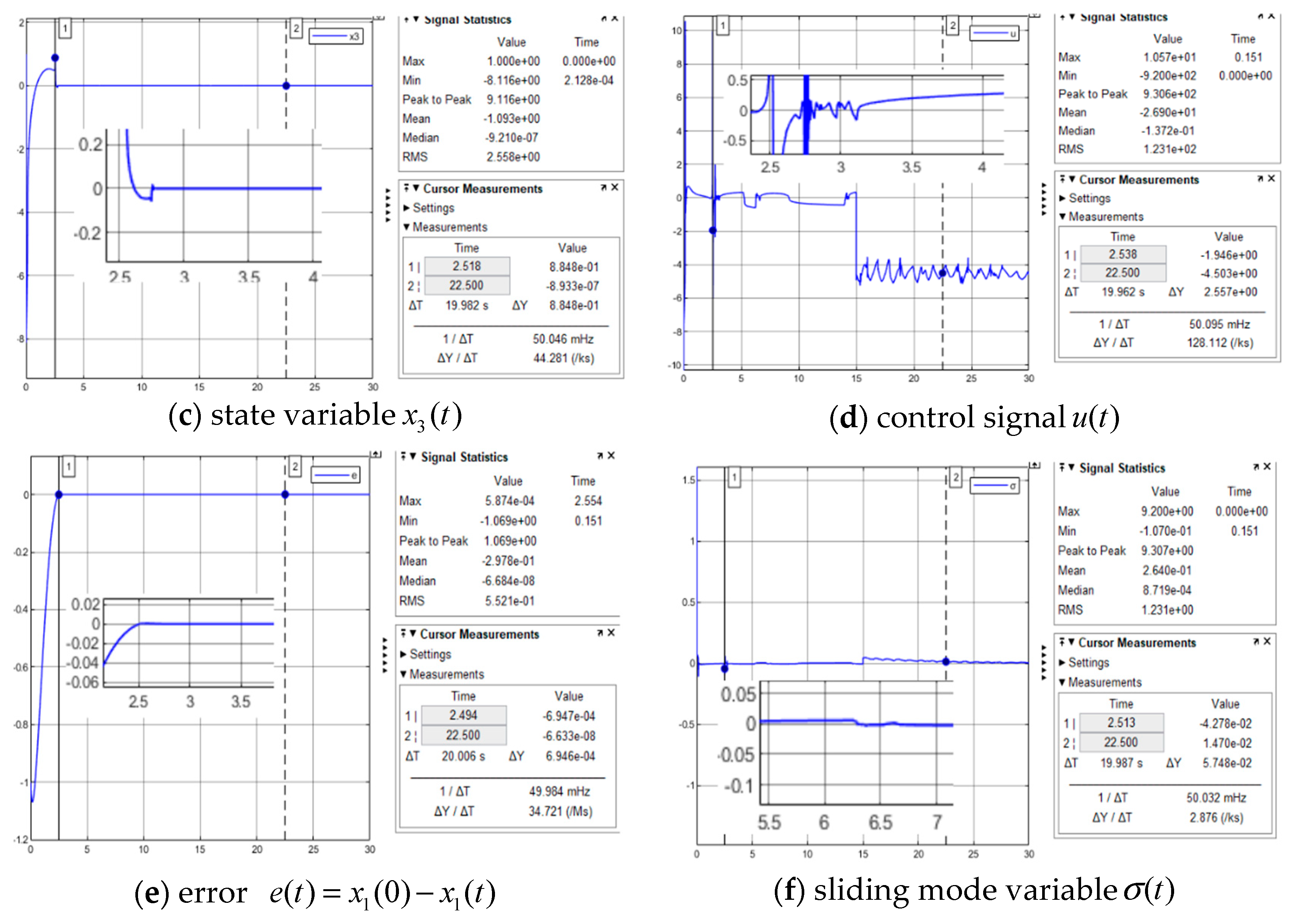
The plots in Figure 5 show off the achieved stabilization of the unstable dynamic plant. The states with transient response and steady errors are achieved from the design objectives. The tracking errors first reach TSM $\sigma =0$ at about $t=0.3$, and then the state vector converges to $x=0$ at about $t$ = 2.5 s.

(2)

Regarding the controller tuning for Figure 5, initially set $\begin{array}{ccc}{k}_g=15,& \begin{array}{cc}{k}_p=15,& k_i=0.8,\end{array}& \delta =1\end{array}$ to establish the system, and fine-tune to $\begin{array}{ccc}{k}_g=10,& \begin{array}{cc}{k}_p=10,& k_i=0.8,\end{array}& \delta =1\end{array}$, while the plots are almost the same within the tested domain of $\begin{array}{ccc}8\le k_g\le 100,& \begin{array}{cc}8\le k_p\le 100,& 0\le k_i\le 2,\end{array}& \delta =1\end{array}$. In case of low gain (not enough strength to keep the control monotonicity), such as gains with $\begin{array}{ccc}{k}_g\le 5,& \begin{array}{cc}{k}_p\le 5,& k_i=0.8,\end{array}& \delta =1\end{array}$, the simulation is stopped by numerical errors.

(3)

There is no singularity problem observed in the operational range, as the MFTSMC is designed without involving the negative derivative of the TSM $u(\dot{\sigma }=0)$.

(4)

Three measures are embedded in the MFTSMC to reduce the chattering effect at the controller output: (a) using the negative definite Lyapunov stability condition $\dot{\sigma }\sigma <0$ rather than model-based negative semi-definite Lyapunov stability condition $\dot{\sigma }=0$; (b) accommodating the system relative degree, where the plant dynamic order is known in the simulation to imply that there is no missed unmodelled dynamic order, and the system relative degree is 3(plant)-2(TSM) = 1 < 3; (c) maintaining the sliding mode boundary thickness $\delta =1$, which does not need to be increased.

(5)

Robustness has been tested in (a) the controller parameter ($k_g,k_p,k_i,\delta$) tuning, as in the Lyapunov differential inequality used in the controller design $u(\dot{\sigma }\sigma <0)$, where there exists a domain satisfying the inequality, for example, ($k_g=20,k_p=20,k_i=5,\delta =1$), (b) plant dynamic variations ($(1\pm 0.5)x_3^3$), and (c) external disturbance rejection, where the same performance is kept as shown in Figure 6. The whole system uncertainty is unknown but bounded. The controller parameter tuning covers the choice to supress the uncertainties to stratify the Lyapunov differential inequality and avoid the chattering effect. The concept of the total robustness controller tuning against plant uncertainties is well demonstrated with the computational experiments. The MFTSMC has much stronger robustness compared with those model-based approaches [5]. This is because of the model-based TSMC using the nominal model. Determining the equivalent control involves the percentage of the uncertainty with ${\displaystyle \frac{\left|UC\right|}{\left|NM\right|+\left|UC\right|}}<100\%$ ($\left|UC\right|$ and $\left|NM\right|$ are the absolute values of uncertainty and nominal model, respectively), and MFTSMC involves ${\displaystyle \frac{\left|NM\right|+\left|UC\right|}{\left|NM\right|+\left|UC\right|}}=100\%$ uncertainty in control.

(6)

For rejection of external disturbance added at the control input, refer to plant (17). The external disturbance in the simulation is considered in the form of $d(t)=100+30\sin (2\pi t)$, entered at the control input at $t=15$, which is the same as that used [5] in attenuating the external disturbance effectively and maintaining the same performance at the state outputs. Figure 6 shows the simulation outcomes.

(7)

In comparison to the results in the other representative work [5], similar, or even better results are obtained. The MFTSMC is simple in design and tuning, and has low cost in controller energy (small gains compared with those used with a value of 500 [5]).

Plant 2: Figure 6 shows the simulated plots. There are several explanations below.

(1)

The same tuning process/observations/discussions are not repeated as those described in the first plant simulation studies. This demonstrates that the MFTMSC is applicable to the nonlinear non-affine system as well.

(2)

For dealing with chattering, the same measures (a) and (b) are kept as with the first system control; (c) enlarge the sliding mode boundary thickness $\delta =10$ starting from $\delta =1$, which has been tested in the range of $\delta =[1,9]$ having chattering with the amplitude $\pm 4$. It is noted that the state vector output is the same in all the tested cases no matter whether chattering appeared or not at the controller output.

(3)

The MFTSMC robustness has been tested again in (a) the controller parameter ($k_g=110,k_p=110,k_i=15,\delta =10$) tuning and (2) plant dynamic variations ($(1\pm 0.5)x_1{x}_2$), in which the same performance is kept as shown in Figure 7.

(4)

Rejection of external disturbance that is the same as used with the first control system, added at the control input. The same satisfactory performance is observed as with those in the first control system. Due to the length of the study, the plots are not shown in the draft.

(5)

While applying the controller with the second plant for both plants, the fact that the same performance was achieved gives further insight that the MFTSMC can be conveniently expanded for switching control, while the whole system switches from plant 1 to plant 2, and vice versa.

Plant 3: Figure 7 shows the simulated plots, which are like those obtained from the representative model-based TSMC [22]. Even though the study is based on single-degree development, it is directly expanded to the two-degree interconnected control system demonstrations with this example. This simulation shows again the similar performance achieved with model-free vs. model-based approaches from plants 1 and 2, in dealing with singularity, chattering, uncertainty, design simplicity, tuning robustness, and robustness against internal uncertainty and external disturbance, suitable for tuning controller parameters on site in real applications (no need to use plant models in the tuning). It should be noted that the appearance of a chattering effect in the control force in Figure 7c comes from the rection to the sinusoidal disturbances ${\tau }_{d1}=2\sin (t)+0.5\sin (200\pi t)$ and ${\tau }_{d2}=\cos (2t)+0.5\sin (200\pi t)$. This case study lays a foundation for the expansion of the SISO MFTSMC to general MIMO systems with coupling and/or underactuated modes.

In summary of the case studies, all three case studies demonstrate the equivalency of model-based approaches and the model-free approach, in terms of sliding mode and Lyapunov stability. The MFTSMC is a supplement to model-based approaches in reducing the request on model quality and enhancing robustness to increase the reliability in operation and recalibration in industrial applications. To overview the design paradigm from the model-based approach (D_mb) to the model-free (D_mf) approach in the whole range of the knowledge spectrum, consider a general expression of aD_mb + bD_mf, a + b = 1, with a = 1 for model-based, 0 < a < 1 for nominal model-based, a = 0 for model-free. The factor a represents the trust in the model fidelity [25]. Obviously, the total model-free approach is more challenging with less knowledge, despite the merits in simplicity and robustness. This is why the total model-free approach has not been properly developed, due to some of the challenges appearing in the study.

6. Conclusions

To rigorously, not merely relying on trial-and-error, configure control systems without a plant physical model and/or data-driven adaptive model, this study provides a showcase by using full state feedback error vector converted TSM and Lyapunov differential inequality-derived monotonically decreasing controllers, plus computational bench validation with three representative examples having analytical and numerical challenges and emerging industrial application potential. This first milestone work establishes a general MFTSMC platform with novelty, challenge, and contribution. This MFTSMC is a supplementary enhancement to the model-based approaches in the interest of improving simplicity, robustness, relieving design dependence on model quality, and narrowing the gap between academic research and applications. In addition, the MFTSMC is intuitively rooted in the bionic; control systems are characterized to mimic human/animal activity or dynamic variation by systematically correcting errors without mathematical models. Surely, the study has also noted the pitfalls and cautions in using the MFTSMC.

For expansion of the study, real bench tests and application demonstrations are on the top of the agenda. Another expansion of the research is to deal with those widely appearing underactuated dynamics in various emerging manmade (engineering) system operations, such as UAV flights, robotic system tracking, bridge crane transportation, and many other mechatronic system missions. Other studies could apply the MFTSMC to some typical control problems such as nonsmoothed nonlinear dynamic systems, switching systems, chaotic systems, and MIMO systems, which have been well researched and applied with model-based paradigms. New total model-free controls will surely enhance these conventional control studies.

References

1. Shtessel, Y.; Edwards, C.; Fridman, L.; Levant, A. Sliding Mode Control and Observation; Birkhauser: New York, NY, USA, 2014. [Google Scholar] [CrossRef]
2. Slotine, J.J.E.; Li, W. Applied Nonlinear Control; Prentice Hall: Hoboken, NJ, USA, 1991. [Google Scholar]
3. Bandyopadhyay, B.; Deepak, F.; Kim, K.S. Sliding Mode Control Using Novel Sliding Surfaces; Springer: Berlin/Heidelberg, Germany, 2009. [Google Scholar]
4. Yu, X.; Feng, Y.; Man, Z. Terminal sliding mode control-An overview. IEEE Open J. Ind. Electron. Soc. 2021, 2, 36–52. [Google Scholar] [CrossRef]
5. Yang, J.; Yu, X.; Zhang, L.; Li, S. A Lyapunov-based approach for recursive continuous higher order nonsingular terminal sliding-mode control. IEEE Trans. Autom. Control 2021, 66, 4424–4431. [Google Scholar] [CrossRef]
6. Yan, X.; Spurgeon, S.K.; Edwards, C. Variable Structure Control of Complex Systems; Communications and Control Engineering; Springer: London, UK, 2017. [Google Scholar]
7. Nasiri, M.; Mobayen, S.; Arzani, A. PID-type terminal sliding mode control for permanent magnet synchronous generator-based enhanced wind energy conversion systems. CSEE J. Power Energy Syst. 2022, 8, 993–1003. [Google Scholar] [CrossRef]
8. Man, Z.; Yu, X. Terminal sliding mode control of MIMO linear systems. IEEE Trans. Circuits Syst. I Regul. Pap. 1997, 44, 1065–1070. [Google Scholar] [CrossRef]
9. Wu, Y.; Yu, X.; Man, Z. Terminal sliding mode control design for uncertain dynamic systems. Syst. Control Lett. 1998, 34, 281–288. [Google Scholar] [CrossRef]
10. Feng, Y.; Yu, X.; Man, Z. Non-singular terminal sliding mode control of rigid manipulators. Automatica 2002, 38, 2159–2167. [Google Scholar] [CrossRef]
11. Feng, Y.; Yu, X.; Han, F. On nonsingular terminal sliding-mode control of nonlinear systems. Automatica 2013, 49, 1715–1722. [Google Scholar] [CrossRef]
12. Hou, Z.; Xiong, S. On model-free adaptive control and its stability analysis. IEEE Trans. Autom. Control 2019, 64, 4555–4569. [Google Scholar] [CrossRef]
13. Castellanos-Cárdenas, D.; Posada, N.L.; Orozco-Duque, A.; Sepúlveda-Cano, L.M.; Castrillón, F.; Camacho, O.E.; Vásquez, R.E. A review on data-driven model-free sliding mode control. Algorithms 2024, 17, 543. [Google Scholar] [CrossRef]
14. Mahalle, M.; Ramezani, A.; Moarefianpour, A. Adaptive terminal sliding mode active fault-tolerant control for a class of uncertain nonlinear systems with application of aircraft wing model with actuator faults. Int. J. Syst. Sci. 2024, 55, 1259–1269. [Google Scholar] [CrossRef]
15. Wang, L.; Chai, T.; Zhai, L. Neural-network-based terminal sliding-mode control of robotic manipulators including actuator dynamics. IEEE Trans. Ind. Electron. 2009, 56, 3296–3304. [Google Scholar] [CrossRef]
16. Chu, Y.; Hou, S.; Fei, J. Continuous terminal sliding mode control using novel fuzzy neural network for active power filter. Control Eng. Pract. 2021, 109, 104735. [Google Scholar] [CrossRef]
17. Zhu, X.; Deng, Y.; Zheng, X.; Zheng, Q.; Liang, B.; Liu, Y. Online reinforcement-learning-based adaptive terminal sliding mode control for disturbed bicycle robots on a curved pavement. Electronics 2022, 11, 3495. [Google Scholar] [CrossRef]
18. Lee, H.; Utkin, V.I. Chattering suppression methods in sliding mode control systems. Annu. Rev. Control 2007, 31, 179–188. [Google Scholar] [CrossRef]
19. Boiko, I.; Fridman, L. Analysis of chattering in continuous sliding-mode controllers. IEEE Trans. Autom. Control 2005, 50, 1442–1446. [Google Scholar] [CrossRef]
20. Seshagiri, S.; Khalil, H.K. On introducing integral action in sliding mode control. In Proceedings of the 41st IEEE Conference on Decision and Control, Las Vegas, NV, USA, 10–13 December 2002; pp. 1473–1478. [Google Scholar] [CrossRef]
21. Pan, Y.; Yang, C.; Pan, L.; Yu, H. Integral Sliding Mode Control: Performance, Modification, and Improvement. IEEE Trans. Ind. Inf. 2018, 14, 3087–3096. [Google Scholar] [CrossRef]
22. Yu, S.; Yu, X.; Shirinzadeh, B.; Man, Z. Continuous finite-time control for robotic manipulators with terminal sliding mode. Automatica 2005, 41, 1957–1964. [Google Scholar] [CrossRef]
23. Pérez-Ventura, U.; Mendoza-Avila, J.; Fridman, L. Design of a proportional integral derivative-like continuous sliding mode controller. Int. J. Robust. Nonlinear Control 2021, 31, 3439–3454. [Google Scholar] [CrossRef]
24. Carvalho, A.D.; Pereira, B.S.; Angélico, B.A.; Laganá, A.A.M.; Justo, J.F. Model-free control applied to a direct injection system: Experimental validation. Fuel 2024, 358 Pt A, 130071. [Google Scholar] [CrossRef]
25. Zhu, Q.; Zhang, W.; Li, S.; Chen, Q.; Na, J.; Ding, H. U-control-a universal platform for control system design with inversion/cancellation of nonlinearity, dynamic and coupling through model-based to model-free procedures. Int. J. Syst. Sci. 2025, 56, 484–501. [Google Scholar] [CrossRef]
26. Gambhire, S.J.; Kishore, D.R.; Londhe, P.S.; Pawar, S.N. Review of sliding mode based control techniques for control system applications. Int. J. Dyn. Control 2021, 9, 363–378. [Google Scholar] [CrossRef]
27. Yu, S.; Wu, H.; Kang, S.; Ma, J.; Xie, M.; Dai, L. Model-free robust motion control for biological optical microscopy using time-delay estimation with an adaptive RBFNN compensator. ISA Trans. 2024, 149, 365–372. [Google Scholar] [CrossRef] [PubMed]
28. Hou, Z.; Yu, X.; Lu, P. Terminal sliding mode control for quadrotors with chattering reduction and disturbances estimator: Theory and application. J. Intell. Robot. Syst. 2022, 105, 71. [Google Scholar] [CrossRef]
29. Mabboux, J.; Pommier-Budinger, V.; Delbecq, S.; Bordeneuve-Guibe, J. Co-design of a multirotor UAV with robust control considering handling qualities and motor failure. Aerosp. Sci. Technol. 2024, 144, 108778. [Google Scholar] [CrossRef]
30. Bhat, S.P.; Bernstein, D.S. Finite-time stability of homogeneous systems. In Proceedings of the 1997 American Control Conference (Cat. No. 97CH36041), Albuquerque, NM, USA, 6 June 1997; pp. 2513–2514. [Google Scholar] [CrossRef]
31. Bhat, S.P.; Bernstein, D.S. Geometric homogeneity with applications to finite-time stability. Math. Control Signals Syst. 2005, 17, 101–127. [Google Scholar] [CrossRef]
32. Karagiannopoulos, S.; Aristidou, P.; Hug, G.; Botterud, A. Decentralized control in active distribution grids via supervised and reinforcement learning. Energy AI 2024, 16, 100342. [Google Scholar] [CrossRef]
33. Guo, B.; Zhao, Z. On the convergence of an extended state observer for nonlinear systems with uncertainty. Syst. Control Lett. 2011, 60, 420–430. [Google Scholar] [CrossRef]
34. Zhu, Q.; Li, R.; Zhang, J. Model-free robust decoupling control of nonlinear nonaffine dynamic systems. Int. J. Syst. Sci. 2023, 54, 2590–2607. [Google Scholar] [CrossRef]
35. Chen, X.; Wang, Y.; Song, Y. Unifying fixed time and prescribed time control for strict-feedback nonlinear systems. IEEE/CAA J. Autom. Sin. 2025, 12, 347–355. [Google Scholar] [CrossRef]
36. Wang, Y.; Gu, L.; Xu, Y.; Cao, X. Practical tracking control of robot manipulators with continuous fractional-order nonsingular terminal sliding mode. IEEE Trans. Ind. Electron. 2016, 63, 6194–6204. [Google Scholar] [CrossRef]
37. Lahiri, A.; Rawat, T.K. Noise analysis of single stage fractional-order low-pass filter using stochastic and fractional Calculus. ECTI Trans. Electr. Eng. Electron. Commun. 2009, 7, 47–54. [Google Scholar] [CrossRef]
38. Liu, W.; Ye, H.; Yang, X. Super-Twisting Sliding Mode Control for the Trajectory Tracking of Underactuated USVs with Disturbances. J. Mar. Sci. Eng. 2023, 11, 636. [Google Scholar] [CrossRef]
39. Zhu, Q. Model-free sliding mode enhanced proportional, integral, and derivative (SMPID) control. Axioms 2023, 12, 721. [Google Scholar] [CrossRef]
40. Yang, I.; Lee, D.; Han, D. Designing a robust nonlinear dynamic inversion controller for spacecraft formation flying. Math. Probl. Eng. 2014, 2014, 471352. [Google Scholar] [CrossRef]
41. Eslami, M. Sensitivity reduction and robustness. In Theory of Sensitivity in Dynamic Systems; Springer: Berlin/Heidelberg, Germany, 1994. [Google Scholar]
42. Zhu, Q.; Na, J.; Zhang, W.; Chen, Q. Total Model-Free Robust Control of Non-Affine Nonlinear Systems with Discontinuous Inputs. Processes 2025, 13, 1315. [Google Scholar] [CrossRef]
43. Iqbal, K. Introduction to Control Systems; University of Ottawa: Ottawa, ON, Canada, 2021. [Google Scholar] [CrossRef]
44. Chen, B.M.; Lee, T.H.; Peng, K.; Venkataramanan, V. Composite nonlinear feedback control for linear systems with input saturation: Theory and an application. IEEE Trans. Autom. Control 2003, 48, 427–439. [Google Scholar] [CrossRef]
45. Rawat, D.; Gupta, M.K.; Sharma, A. Intelligent control of robotic manipulators: A comprehensive review. Spat. Inf. Res. 2023, 31, 345–357. [Google Scholar] [CrossRef]
Figure 1. Model-based SMC.
Mathematics 13 01559 g001
Figure 2. Total model-free SMC.
Mathematics 13 01559 g002
Figure 3. MFTSMC system.
Mathematics 13 01559 g003
Figure 4. Two-link rigid robotic manipulator.
Mathematics 13 01559 g004
Figure 5. MFTSMC—plant 1.
Mathematics 13 01559 g005
Figure 6. MFTSMC—plant 2.
Mathematics 13 01559 g006aMathematics 13 01559 g006b
Figure 7. MFTSMC—plant 3.
Mathematics 13 01559 g007