
Improving Portfolio Management Using Clustering and Particle Swarm Optimisation


Abstract
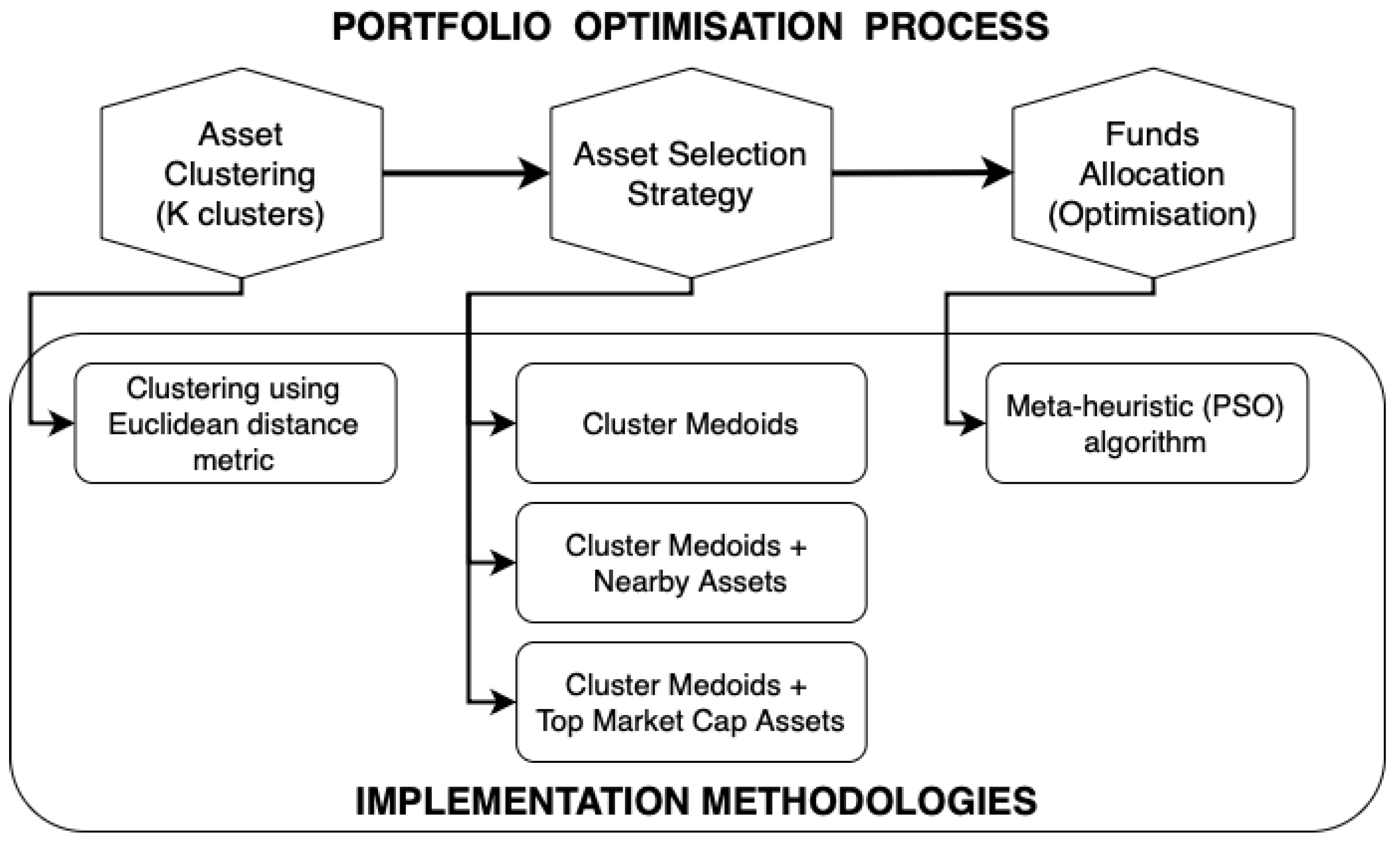
1. Introduction
- RQ1: To what extent do different smoothing techniques influence risk-adjusted returns of single-asset-type portfolios of different asset classes?
- RQ2: Which selection criteria best identify representative assets from clusters formed using risk–return characteristics of smoothed data?
2. Related Work
2.1. Traditional Portfolio Optimisation Techniques
2.1.1. Markowitz Mean–Variance (MV) Theory
2.1.2. Sharpe and Sortino Ratio
2.2. Portfolio Optimisation Using Meta-Heuristic Algorithms
2.3. Clustering of Financial Assets
3. Data Handling and Asset Selection Strategies
3.1. Dataset Description
3.2. Dataset Preprocessing
3.2.1. Handling Missing Values
3.2.2. Implementation of Smoothing Algorithms
3.3. Meta-Heuristic Algorithm Used for Portfolio Optimisation—Particle Swarm Optimisation
- represent dimensions; represent the particle;
- N is the size of the swarm, i.e., the total number of particles; is the inertia weight;
- are two positive constants, called the cognitive and social parameters, respectively;
- are random numbers, uniformly distributed in ;
- g is the index of the overall best particle in the swarm; and
- determines the iteration number of the algorithm.
- represent dimensions; represent particles;
- N is the size of the swarm, i.e., total number of particles;
- is called compression–expansion coefficient;
- is a random number from a standard normal distribution ; and
- is mean best (), i.e., average of of all particles at iteration t, i.e.,
3.4. K-Medoids-Based Clustering and Optimal Selection of Financial Assets
4. Results
4.1. Missing Value Handling Techniques
4.2. Analysis of Different Smoothing Strategies
4.3. Hyperparameter Optimisation for the Particle Swarm Optimisation (PSO) Algorithm
4.4. Benchmarking PSO with Previous Works
4.5. Analysis of the Effects of Clustering and Different Asset Selection Techniques
4.5.1. Comparison of the Effects of Clustering and Asset Selection Strategy with the Non-Clustered Approach on the Corresponding Portfolios
4.5.2. Comparison of Different PSO Techniques
4.5.3. Comparison of Different Asset Selection Strategies
4.6. Benchmarking with Literature Review
5. Discussion and Conclusions
6. Future Work
Author Contributions
Funding
Data Availability Statement
Acknowledgments
Conflicts of Interest
Appendix A. Subset of Assets Used

| Top 10 Crypto Coins | Top 20 S&P Stocks | Top 20 S&P Stocks |
|---|---|---|
| Bitcoin (BTC) | MICROSOFT CORP (MSFT) | APPLE INC (AAPL) |
| Ethereum (ETH) | NVIDIA CORP (NVDA) | AMAZON.COM, INC (AMZN) |
| Tether (USDT) | META PLATFORMS INC, CLASS A (META) | ALPHABET INC CL C (GOOG) |
| Ripple (XRP) | BERKSHIRE HATHAWAY INC. CL B (BRK.B) | ELI LILLY AND COMPANY (LLY) |
| USD Coin (USDC) | BROADCOM INC. (AVGO) | TESLA, INC (TSLA) |
| Dogecoin (DOGE) | JPMORGAN CHASE & COMPANY (JPM) | UNITEDHEALTH GROUP INC (UNH) |
| Cardano (ADA) | VISA INC. (V) | EXXON MOBIL CORP (XOM) |
| Tron (TRX) | JOHNSON & JOHNSON (JNJ) | MASTERCARD INC (MA) |
| Litecoin (LTC) | THE PROCTER & GAMBLE COMPANY (PG) | HOME DEPOT, INC. (HD) |
| Dai (DAI) | MERCK COMPANY. INC. (MRK) | COSTCO WHOLESALE CORP (COST) |
Appendix B. Pseudocodes
Appendix B.1
| Algorithm A1: Standard Particle Swarm Optimisation (SPSO) Algorithm |
 |
Appendix B.2
| Algorithm A2: K-Medoids Clustering Algorithm |
 |
References
- Ta, V.D.; Liu, C.M.; Tadesse, D.A. Portfolio Optimization-Based Stock Prediction Using Long-Short Term Memory Network in Quantitative Trading. Appl. Sci. 2020, 10, 437. [Google Scholar] [CrossRef]
- Markowitz, H.M. Portfolio Selection: Efficient Diversification of Investments; J. Wiley: Hoboken, NJ, USA, 1959. [Google Scholar]
- Sharpe, W.F. Capital Asset Prices: A Theory of Market Equilibrium Under Conditions of Risk. J. Financ. 1964, 19, 425–442. [Google Scholar] [CrossRef]
- Rockafellar, R.T.; Uryasev, S. Optimization of conditional value-at-risk. J. Risk 2000, 2, 21–41. [Google Scholar] [CrossRef]
- Golmakani, H.R.; Fazel, M. Constrained Portfolio Selection using Particle Swarm Optimization. Expert Syst. Appl. 2011, 38, 8327–8335. [Google Scholar] [CrossRef]
- Niu, B.; Fan, Y.; Xiao, H.; Xue, B. Bacterial foraging based approaches to portfolio optimization with liquidity risk. Neurocomputing 2012, 98, 90–100. [Google Scholar] [CrossRef]
- Metaxiotis, K.; Liagkouras, K. Multiobjective Evolutionary Algorithms for Portfolio Management: A comprehensive literature review. Expert Syst. Appl. 2012, 39, 11685–11698. [Google Scholar] [CrossRef]
- Aithal, P.K.; Geetha, M.; U, D.; Savitha, B.; Menon, P. Real-Time Portfolio Management System Utilizing Machine Learning Techniques. IEEE Access 2023, 11, 32545–32559. [Google Scholar] [CrossRef]
- Gunjan, A.; Bhattacharyya, S. A brief review of portfolio optimization techniques. Artif. Intell. Rev. 2023, 56, 3847–3886. [Google Scholar] [CrossRef]
- Grinold, R.C.; Kahn, R.N. Active Portfolio Management; McGraw-Hill: New York, NY, USA, 2000. [Google Scholar]
- El Bernoussi, R.; Rockinger, M. Rebalancing with transaction costs: Theory, simulations, and actual data. Financ. Mark. Portf. Manag. 2023, 37, 121–160. [Google Scholar] [CrossRef]
- S, K. Security Analysis and Portfolio Management, 3rd ed.; PHI Learning Pvt. Ltd.: Delhi, India, 2022. [Google Scholar]
- Thakkar, A.; Chaudhari, K. A Comprehensive Survey on Portfolio Optimization, Stock Price and Trend Prediction Using Particle Swarm Optimization. Arch. Comput. Methods Eng. 2021, 28, 2133–2164. [Google Scholar] [CrossRef]
- Nti, I.K.; Adekoya, A.F.; Weyori, B.A. A systematic review of fundamental and technical analysis of stock market predictions. Artif. Intell. Rev. 2020, 53, 3007–3057. [Google Scholar] [CrossRef]
- Thakkar, A.; Chaudhari, K. CREST: Cross-Reference to Exchange-based Stock Trend Prediction using Long Short-Term Memory. Procedia Comput. Sci. 2020, 167, 616–625. [Google Scholar] [CrossRef]
- Anbalagan, T.; Maheswari, S.U. Classification and Prediction of Stock Market Index Based on Fuzzy Metagraph. Procedia Comput. Sci. 2015, 47, 214–221. [Google Scholar] [CrossRef]
- Wen, Q.; Yang, Z.; Song, Y.; Jia, P. Automatic stock decision support system based on box theory and SVM algorithm. Expert Syst. Appl. 2010, 37, 1015–1022. [Google Scholar] [CrossRef]
- Raudys, A.; Lenčiauskas, V.; Malčius, E. Moving averages for financial data smoothing. In Proceedings of the Information and Software Technologies: 19th International Conference, ICIST 2013, Kaunas, Lithuania, 10–11 October 2013; Proceedings 19. Springer: Berlin/Heidelberg, Germany, 2013; pp. 34–45. [Google Scholar]
- Cesarone, F.; Scozzari, A.; Tardella, F. A new method for mean-variance portfolio optimization with cardinality constraints. Ann. Oper. Res. 2013, 205, 213–234. [Google Scholar] [CrossRef]
- Lim, Q.Y.E.; Cao, Q.; Quek, C. Dynamic portfolio rebalancing through reinforcement learning. Neural Comput. Appl. 2022, 34, 7125–7139. [Google Scholar] [CrossRef]
- Ma, Y.; Ahmad, F.; Liu, M.; Wang, Z. Portfolio optimization in the era of digital financialization using cryptocurrencies. Technol. Forecast. Soc. Change 2020, 161, 120265. [Google Scholar] [CrossRef] [PubMed]
- Lorenzo, L.; Arroyo, J. Online risk-based portfolio allocation on subsets of crypto assets applying a prototype-based clustering algorithm. Financ. Innov. 2023, 9, 25. [Google Scholar] [CrossRef]
- Menvouta, E.J.; Serneels, S.; Verdonck, T. Portfolio optimization using cellwise robust association measures and clustering methods with application to highly volatile markets. J. Financ. Data Sci. 2023, 9, 100097. [Google Scholar] [CrossRef]
- Maghsoodi, A.I. Cryptocurrency portfolio allocation using a novel hybrid and predictive big data decision support system. Omega 2023, 115, 102787. [Google Scholar] [CrossRef]
- McMillan, D.G. Cross-asset relations, correlations and economic implications. Glob. Financ. J. 2019, 41, 60–78. [Google Scholar] [CrossRef]
- Zeevi, A.; Mashal, R. Beyond Correlation: Extreme Co-Movements Between Financial Assets. Available at SSRN 317122. 2002. Available online: https://ssrn.com/abstract=317122 (accessed on 20 March 2025).
- Koumou, G.B. Diversification and portfolio theory: A review. Financ. Mark. Portf. Manag. 2020, 34, 267–312. [Google Scholar] [CrossRef]
- Tolun Tayalı, S. A novel backtesting methodology for clustering in mean–variance portfolio optimization. Knowl.-Based Syst. 2020, 209, 106454. [Google Scholar] [CrossRef]
- U.S. Department of the Treasury. Available online: https://home.treasury.gov/resource-center/data-chart-center/interest-rates/TextView?type=daily_treasury_bill_rates&field_tdr_date_value=2023 (accessed on 9 April 2024).
- Zhu, H.; Wang, Y.; Wang, K.; Chen, Y. Particle Swarm Optimization (PSO) for the constrained portfolio optimization problem. Expert Syst. Appl. 2011, 38, 10161–10169. [Google Scholar] [CrossRef]
- Zaheer, K.B.; Abd Aziz, M.I.B.; Kashif, A.N.; Raza, S.M.M. Two stage portfolio selection and optimization model with the hybrid particle swarm optimization. Matematika 2018, 34, 125–141. [Google Scholar] [CrossRef]
- Sun, J.; Fang, W.; Wu, X.; Lai, C.H.; Xu, W. Solving the multi-stage portfolio optimization problem with a novel particle swarm optimization. Expert Syst. Appl. 2011, 38, 6727–6735. [Google Scholar] [CrossRef]
- Sortino, F.A.; Price, L.N. Performance measurement in a downside risk framework. J. Invest. 1994, 3, 59–64. [Google Scholar] [CrossRef]
- Bailey, D.H.; Lopez de Prado, M. The Sharpe ratio efficient frontier. J. Risk 2012, 15, 13. [Google Scholar] [CrossRef]
- Mistry, J.; Shah, J. Dealing with the limitations of the Sharpe ratio for portfolio evaluation. J. Commer. Account. Res. 2013, 2, 10. [Google Scholar]
- Cuchieri, N. Deep Reinforcement Learning for Financial Portfolio Optimisation. Master’s Thesis, University of Malta, Msida, Malta, 2021. [Google Scholar]
- Sharma, A.; Mehra, A. Financial analysis based sectoral portfolio optimization under second order stochastic dominance. Ann. Oper. Res. 2017, 256, 171–197. [Google Scholar] [CrossRef]
- Chang, T.J.; Meade, N.; Beasley, J.E.; Sharaiha, Y.M. Heuristics for cardinality constrained portfolio optimisation. Comput. Oper. Res. 2000, 27, 1271–1302. [Google Scholar] [CrossRef]
- Schaerf, A. Local Search Techniques for Constrained Portfolio Selection Problems. Comput. Econ. 2002, 20, 177–190. [Google Scholar] [CrossRef]
- Kennedy, J.; Eberhart, R. Particle swarm optimization. In Proceedings of the ICNN’95—International Conference on Neural Networks, Perth, WA, Australia, 27 November–1 December 1995; Volume 4, pp. 1942–1948. [Google Scholar] [CrossRef]
- Dorigo, M.; Maniezzo, V.; Colorni, A. Ant system: Optimization by a colony of cooperating agents. IEEE Trans. Syst. Man Cybern. Part B (Cybern.) 1996, 26, 29–41. [Google Scholar] [CrossRef]
- Vikhar, P.A. Evolutionary algorithms: A critical review and its future prospects. In Proceedings of the 2016 International Conference on Global Trends in Signal Processing, Information Computing and Communication (ICGTSPICC), Jalgaon, India, 22–24 December 2016; pp. 261–265. [Google Scholar]
- Lin, T.L.; Horng, S.J.; Kao, T.W.; Chen, Y.H.; Run, R.S.; Chen, R.J.; Lai, J.L.; Kuo, I.H. An efficient job-shop scheduling algorithm based on particle swarm optimization. Expert Syst. Appl. 2010, 37, 2629–2636. [Google Scholar] [CrossRef]
- Nguyen, S.; Zhang, M.; Johnston, M.; Tan, K.C. Automatic Programming via Iterated Local Search for Dynamic Job Shop Scheduling. IEEE Trans. Cybern. 2015, 45, 1–14. [Google Scholar] [CrossRef] [PubMed]
- Chernbumroong, S.; Cang, S.; Yu, H. Genetic Algorithm-Based Classifiers Fusion for Multisensor Activity Recognition of Elderly People. IEEE J. Biomed. Health Inform. 2015, 19, 282–289. [Google Scholar] [CrossRef] [PubMed]
- Chen, C.H.; Liu, T.K.; Chou, J.H. A Novel Crowding Genetic Algorithm and Its Applications to Manufacturing Robots. IEEE Trans. Ind. Inform. 2014, 10, 1705–1716. [Google Scholar] [CrossRef]
- Yang, X.S.; Talatahari, S.; Alavi, A.H. Metaheuristic Applications in Structures and Infrastructures; Elsevier: Waltham, MA, USA, 2013. [Google Scholar]
- Ertenlice, O.; Kalayci, C.B. A survey of swarm intelligence for portfolio optimization: Algorithms and applications. Swarm Evol. Comput. 2018, 39, 36–52. [Google Scholar] [CrossRef]
- Chen, Y.; Zhao, X.; Yuan, J. Swarm intelligence algorithms for portfolio optimization problems: Overview and recent advances. Mob. Inf. Syst. 2022, 2022, 4241049. [Google Scholar] [CrossRef]
- Erwin, K.; Engelbrecht, A. Meta-heuristics for portfolio optimization. Soft Comput. 2023, 27, 19045–19073. [Google Scholar] [CrossRef]
- Leung, M.F.; Wang, J. Minimax and biobjective portfolio selection based on collaborative neurodynamic optimization. IEEE Trans. Neural Netw. Learn. Syst. 2020, 32, 2825–2836. [Google Scholar] [CrossRef] [PubMed]
- Deng, G.F.; Lin, W.T.; Lo, C.C. Markowitz-based portfolio selection with cardinality constraints using improved particle swarm optimization. Expert Syst. Appl. 2012, 39, 4558–4566. [Google Scholar] [CrossRef]
- Wang, W.; Wang, H.; Wu, Z.; Dai, H. A Simple and Fast Particle Swarm Optimization and Its Application on Portfolio Selection. In Proceedings of the 2009 International Workshop on Intelligent Systems and Applications, Wuhan, China, 23–24 May 2009; pp. 1–4. [Google Scholar] [CrossRef]
- Yin, X.; Ni, Q.; Zhai, Y. A novel PSO for portfolio optimization based on heterogeneous multiple population strategy. In Proceedings of the 2015 IEEE Congress on Evolutionary Computation (CEC), Sendai, Japan, 25–28 May 2015; pp. 1196–1203. [Google Scholar] [CrossRef]
- Chen, C.; Chen, B.y. Complex portfolio selection using improving particle swarm optimization approach. In Proceedings of the 2018 IEEE 20th International Conference on High Performance Computing and Communications; IEEE 16th International Conference on Smart City; IEEE 4th International Conference on Data Science and Systems (HPCC/SmartCity/DSS), Exeter, UK, 28–30 June 2018; pp. 828–835. [Google Scholar]
- Koshino, M.; Murata, H.; Kimura, H. Improved particle swarm optimization and application to portfolio selection. Electron. Commun. Jpn. (Part III Fundam. Electron. Sci.) 2007, 90, 13–25. [Google Scholar] [CrossRef]
- Ponsich, A.; Jaimes, A.L.; Coello, C.A.C. A survey on multiobjective evolutionary algorithms for the solution of the portfolio optimization problem and other finance and economics applications. IEEE Trans. Evol. Comput. 2012, 17, 321–344. [Google Scholar] [CrossRef]
- Yu, L.; Wang, S.; Lai, K.K. Portfolio optimization using evolutionary algorithms. In Reflexing Interfaces: The Complex Coevolution of Information Technology Ecosystems; IGI Global: Hershey, PA, USA, 2008; pp. 235–245. [Google Scholar]
- Chen, A.H.L.; Liang, Y.C.; Liu, C.C. Portfolio optimization using improved artificial bee colony approach. In Proceedings of the 2013 IEEE Conference on Computational Intelligence for Financial Engineering & Economics (CIFEr), Singapore, 16–19 April 2013; pp. 60–67. [Google Scholar] [CrossRef]
- Kalayci, C.B.; Polat, O.; Akbay, M.A. An efficient hybrid metaheuristic algorithm for cardinality constrained portfolio optimization. Swarm Evol. Comput. 2020, 54, 100662. [Google Scholar] [CrossRef]
- Machdar, N.M. The Effect of Capital Structure, Systematic Risk, and Unsystematic Risk on Stock Return. Bus. Entrep. Rev. 2015, 14, 149–160. [Google Scholar] [CrossRef]
- Rodriguez, M.Z.; Comin, C.H.; Casanova, D.; Bruno, O.M.; Amancio, D.R.; Costa, L.d.F.; Rodrigues, F.A. Clustering algorithms: A comparative approach. PLoS ONE 2019, 14, e0210236. [Google Scholar] [CrossRef] [PubMed]
- Sarker, I.H. Machine learning: Algorithms, real-world applications and research directions. SN Comput. Sci. 2021, 2, 160. [Google Scholar] [CrossRef]
- Tenkam, H.M.; Mba, J.C.; Mwambi, S.M. Optimization and Diversification of Cryptocurrency Portfolios: A Composite Copula-Based Approach. Appl. Sci. 2022, 12, 6408. [Google Scholar] [CrossRef]
- Rdusseeun, L.; Kaufman, P. Clustering by means of medoids. In Proceedings of the Statistical Data Analysis Based on the L1 Norm Conference, Neuchatel, Switzerland, 31 August–4 September 1987; Volume 31. [Google Scholar]
- Duarte, F.G.; De Castro, L.N. A Framework to Perform Asset Allocation Based on Partitional Clustering. IEEE Access 2020, 8, 110775–110788. [Google Scholar] [CrossRef]
- Arora, P.; Deepali; Varshney, S. Analysis of K-Means and K-Medoids Algorithm For Big Data. Procedia Comput. Sci. 2016, 78, 507–512. [Google Scholar] [CrossRef]
- Cui, X.; Sun, X.; Zhu, S.; Jiang, R.; Li, D. Portfolio optimization with nonparametric value at risk: A block coordinate descent method. INFORMS J. Comput. 2018, 30, 454–471. [Google Scholar] [CrossRef]
- Lopez de Prado, M. Building diversified portfolios that outperform out-of-sample. J. Portf. Manag. 2016, 42, 59–69. [Google Scholar] [CrossRef]
- Sass, J.; Thös, A.K. Risk reduction and portfolio optimization using clustering methods. Econom. Stat. 2024, 32, 1–16. [Google Scholar] [CrossRef]
- U, I.; Yun, I.; Jong, H.; Rim, W. Portfolio Optimization Based on K-Means Clustering and Particle Swarm Optimization Using Financial Statements and Stock Price Data. Available online: https://ssrn.com/abstract=4937613 (accessed on 28 March 2025).
- Bjerring, T.T.; Ross, O.; Weissensteiner, A. Feature selection for portfolio optimization. Ann. Oper. Res. 2017, 256, 21–40. [Google Scholar] [CrossRef]
- Nanda, S.R.; Mahanty, B.; Tiwari, M.K. Clustering Indian stock market data for portfolio management. Expert Syst. Appl. 2010, 37, 8793–8798. [Google Scholar] [CrossRef]
- Bezdek, J.C.; Pal, N.R. Cluster validation with generalized Dunn’s indices. In Proceedings of the 1995 Second New Zealand International Two-Stream Conference on Artificial Neural Networks and Expert Systems, Dunedin, New Zealand, 20–23 November 1995; pp. 190–193. [Google Scholar]
- Navarro, M.M.; Young, M.N.; Prasetyo, Y.T.; Taylar, J.V. Stock market optimization amidst the COVID-19 pandemic: Technical analysis, K-means algorithm, and mean-variance model (TAKMV) approach. Heliyon 2023, 9, e17577. [Google Scholar] [CrossRef]
- Wu, D.; Wang, X.; Wu, S. Construction of stock portfolios based on k-means clustering of continuous trend features. Knowl.-Based Syst. 2022, 252, 109358. [Google Scholar] [CrossRef]
- Chen, R.R.; Huang, W.K.; Yeh, S.K. Particle swarm optimization approach to portfolio construction. Intell. Syst. Account. Financ. Manag. 2021, 28, 182–194. [Google Scholar] [CrossRef]
- Data, F. Complete Intraday Bundle. Available online: https://firstratedata.com/cb/1/complete-us-stocks-index-etf-futures (accessed on 30 April 2023).
- Platanakis, E.; Urquhart, A. Should investors include bitcoin in their portfolios? A portfolio theory approach. Br. Account. Rev. 2020, 52, 100837. [Google Scholar] [CrossRef]
- Federal Reserve Bank of St. Louis. 3-Month Treasury Bill Secondary Market Rate, Discount Basis (TB3MS). Available online: https://fred.stlouisfed.org/series/TB3MS#0 (accessed on 30 May 2023).
- Top 25 Stocks in the S&P 500 By Index Weight for March 2025. Available online: https://www.investopedia.com/best-25-sp500-stocks-8550793 (accessed on 9 April 2024).
- Elton, E.J. Presidential Address: Expected Return, Realized Return, and Asset Pricing Tests. J. Financ. 1999, 54, 1199–1220. [Google Scholar] [CrossRef]
- Daily Returns Meaning. Available online: https://www.stockopedia.com/ratios/daily-volatility-12000/ (accessed on 5 October 2024).
- Peng, J.; Hahn, J.; Huang, K.W. Handling missing values in information systems research: A review of methods and assumptions. Inf. Syst. Res. 2023, 34, 5–26. [Google Scholar] [CrossRef]
- Pratama, I.; Permanasari, A.E.; Ardiyanto, I.; Indrayani, R. A review of missing values handling methods on time-series data. In Proceedings of the 2016 International Conference on Information Technology Systems and Innovation (ICITSI), Bandung, Indonesia, 24–27 October 2016; pp. 1–6. [Google Scholar]
- Uddin, A.; Tao, X.; Chou, C.C.; Yu, D. Are missing values important for earnings forecasts? A machine learning perspective. Quant. Financ. 2022, 22, 1113–1132. [Google Scholar] [CrossRef] [PubMed]
- Kofman, P.; Sharpe, I.G. Using multiple imputation in the analysis of incomplete observations in finance. J. Financ. Econom. 2003, 1, 216–249. [Google Scholar] [CrossRef]
- Chen, A.Y.; McCoy, J. Missing values handling for machine learning portfolios. J. Financ. Econ. 2024, 155, 103815. [Google Scholar] [CrossRef]
- Wang, C.H.; Zeng, Y.; Yuan, J. Two-stage stock portfolio optimization based on AI-powered price prediction and mean-CVaR models. Expert Syst. Appl. 2024, 255, 124555. [Google Scholar] [CrossRef]
- Ojha, A.; Saxena, V. Understanding stock market trends using simple moving average (SMA) and exponential moving average (EMA) indicators. In Proceedings of the 2023 6th International Conference on Contemporary Computing and Informatics (IC3I), Gautam Buddha Nagar, India, 14–16 September 2023; Volume 6, pp. 1931–1935. [Google Scholar]
- Time Series and Moving Averages. Available online: https://www.accaglobal.com/ie/en/student/exam-support-resources/fundamentals-exams-study-resources/f5/technical-articles/time-series.html#:%5C~:text=The%5C%20first%5C%20four%5C%20observations%5C%20are,together%5C%20and%5C%20dividing%5C%20by%5C%20two (accessed on 20 October 2024).
- Amal, M.A.; Napitupulu, H.; Sukono. Particle Swarm Optimization Algorithm for Determining Global Optima of Investment Portfolio Weight Using Mean-Value-at-Risk Model in Banking Sector Stocks. Mathematics 2024, 12, 3920. [Google Scholar] [CrossRef]
- Xu, F.; Chen, W.; Yang, L. Improved Particle Swarm Optimization for Realistic Portfolio Selection. In Proceedings of the Eighth ACIS International Conference on Software Engineering, Artificial Intelligence, Networking, and Parallel/Distributed Computing (SNPD 2007), Qingdao, China, 30 July–1 August 2007; Volume 1, pp. 185–190. [Google Scholar] [CrossRef]
- Črepinšek, M.; Liu, S.H.; Mernik, M. Exploration and exploitation in evolutionary algorithms: A survey. ACM Comput. Surv. (CSUR) 2013, 45, 1–33. [Google Scholar] [CrossRef]
- Freitas, D.; Lopes, L.G.; Morgado-Dias, F. Particle swarm optimisation: A historical review up to the current developments. Entropy 2020, 22, 362. [Google Scholar] [CrossRef]
- Mean-Variance Optimization. Available online: https://pyportfolioopt.readthedocs.io/en/latest/MeanVariance.html (accessed on 20 July 2023).
- Jensen, T.I.; Kelly, B.T.; Malamud, S.; Pedersen, L.H. Machine Learning and the Implementable Efficient Frontier. Swiss Finance Institute Research Paper. 2024. Available online: https://ssrn.com/abstract=4187217 (accessed on 20 March 2025).
- Merton, R.C. An analytic derivation of the efficient portfolio frontier. J. Financ. Quant. Anal. 1972, 7, 1851–1872. [Google Scholar] [CrossRef]
- General Efficient Frontier. Available online: https://pyportfolioopt.readthedocs.io/en/latest/GeneralEfficientFrontier.html (accessed on 15 July 2023).
- Lorenzo, L.; Arroyo, J. Analysis of the cryptocurrency market using different prototype-based clustering techniques. Financ. Innov. 2022, 8, 7. [Google Scholar] [CrossRef]
- Rousseeuw, P.J. Silhouettes: A graphical aid to the interpretation and validation of cluster analysis. J. Comput. Appl. Math. 1987, 20, 53–65. [Google Scholar] [CrossRef]
- Thorndike, R.L. Who belongs in the family? Psychometrika 1953, 18, 267–276. [Google Scholar] [CrossRef]
- Shutaywi, M.; Kachouie, N.N. Silhouette analysis for performance evaluation in machine learning with applications to clustering. Entropy 2021, 23, 759. [Google Scholar] [CrossRef]
- sklearn Extra K-Medoids. Available online: https://scikit-learn-extra.readthedocs.io/en/stable/generated/sklearn_extra.cluster.KMedoids.html (accessed on 9 October 2024).
- Understanding Small-Cap and Big-Cap Stocks. Available online: https://www.investopedia.com/insights/understanding-small-and-big-cap-stocks/ (accessed on 12 October 2024).
- Sanderson, R.; Lumpkin-Sowers, N.L. Buy and hold in the new age of stock market volatility: A story about ETFs. Int. J. Financ. Stud. 2018, 6, 79. [Google Scholar] [CrossRef]
- Evans, J.L. The random walk hypothesis, portfolio analysis and the buy-and-hold criterion. J. Financ. Quant. Anal. 1968, 3, 327–342. [Google Scholar] [CrossRef]
- Paiva, F.D.; Cardoso, R.T.N.; Hanaoka, G.P.; Duarte, W.M. Decision-making for financial trading: A fusion approach of machine learning and portfolio selection. Expert Syst. Appl. 2019, 115, 635–655. [Google Scholar] [CrossRef]
- Nzokem, A.; Maposa, D. Bitcoin versus s&p 500 index: Return and risk analysis. Math. Comput. Appl. 2024, 29, 44. [Google Scholar]
- Caferra, R.; Vidal-Tomás, D. Who raised from the abyss? A comparison between cryptocurrency and stock market dynamics during the COVID-19 pandemic. Financ. Res. Lett. 2021, 43, 101954. [Google Scholar] [CrossRef]
- Brini, A.; Lenz, J. A comparison of cryptocurrency volatility-benchmarking new and mature asset classes. Financ. Innov. 2024, 10, 122. [Google Scholar] [CrossRef]
- Alonso-Monsalve, S.; Suárez-Cetrulo, A.L.; Cervantes, A.; Quintana, D. Convolution on neural networks for high-frequency trend prediction of cryptocurrency exchange rates using technical indicators. Expert Syst. Appl. 2020, 149, 113250. [Google Scholar] [CrossRef]
- Source Code for Efficient Frontier Class in Python. Available online: https://pyportfolioopt.readthedocs.io/en/latest/_modules/pypfopt/efficient_frontier/efficient_frontier.html (accessed on 9 October 2024).
- Aljinović, Z.; Marasović, B.; Šestanović, T. Cryptocurrency portfolio selection—A multicriteria approach. Mathematics 2021, 9, 1677. [Google Scholar] [CrossRef]
- CoinMarketCap—Cryptocurrency Prices by Market Cap. Available online: https://coinmarketcap.com (accessed on 7 July 2024).
- The 100 Largest Companies in the World by Market Capitalization in 2024. Available online: https://www.statista.com/statistics/263264/top-companies-in-the-world-by-market-capitalization/ (accessed on 12 January 2025).
- Kim, Y.B.; Kim, J.G.; Kim, W.; Im, J.H.; Kim, T.H.; Kang, S.J.; Kim, C.H. Predicting fluctuations in cryptocurrency transactions based on user comments and replies. PLoS ONE 2016, 11, e0161197. [Google Scholar] [CrossRef] [PubMed]


| Stocks Only | |||
|---|---|---|---|
| SPSO | IPSO | DPSO | Paper |
| 4.8832 | 4.8802 | 4.8843 | 1.27 |
 |
Disclaimer/Publisher’s Note: The statements, opinions and data contained in all publications are solely those of the individual author(s) and contributor(s) and not of MDPI and/or the editor(s). MDPI and/or the editor(s) disclaim responsibility for any injury to people or property resulting from any ideas, methods, instructions or products referred to in the content. |
© 2025 by the authors. Licensee MDPI, Basel, Switzerland. This article is an open access article distributed under the terms and conditions of the Creative Commons Attribution (CC BY) license (https://creativecommons.org/licenses/by/4.0/).
Share and Cite
Bulani, V.; Bezbradica, M.; Crane, M. Improving Portfolio Management Using Clustering and Particle Swarm Optimisation. Mathematics 2025, 13, 1623. https://doi.org/10.3390/math13101623
Bulani V, Bezbradica M, Crane M. Improving Portfolio Management Using Clustering and Particle Swarm Optimisation. Mathematics. 2025; 13(10):1623. https://doi.org/10.3390/math13101623
Chicago/Turabian StyleBulani, Vivek, Marija Bezbradica, and Martin Crane. 2025. "Improving Portfolio Management Using Clustering and Particle Swarm Optimisation" Mathematics 13, no. 10: 1623. https://doi.org/10.3390/math13101623
APA StyleBulani, V., Bezbradica, M., & Crane, M. (2025). Improving Portfolio Management Using Clustering and Particle Swarm Optimisation. Mathematics, 13(10), 1623. https://doi.org/10.3390/math13101623