Stability and Performance Analysis of Single-Step FCS-MPC System Based on Regional ISS Theory

Abstract

In recent years, finite-control-set model predictive control (FCS-MPC) has attracted significant attention in power electronic converter control, resulting in substantial research advancements. However, no formal method currently exists to prove the stability of FCS-MPC systems. Additionally, many application studies have yet to adequately address the relationship between the selection of design parameters and system performance. To address the lack of stability and performance guarantees in FCS-MPC system design, this paper investigates a class of single-step FCS-MPC systems. The analysis is based on regional input-to-state stability (ISS) theory. Sufficient conditions for ensuring regional stability are derived, and a method for estimating the system’s domain of attraction and ultimate bounded region is developed. Simulation experiments validated the analytical results and revealed the relationships between the domain of attraction and system stability, as well as between the ultimate bounded region and steady-state performance. The results indicate that appropriate parameter design can ensure system stability. Furthermore, the proposed method elucidates how changes in design parameters affect system stability and steady-state performance, providing a theoretical foundation for designing a class of FCS-MPC systems.

1. Introduction

Finite-control-set model predictive control (FCS-MPC) is a special form of model predictive control (MPC) characterized by restricting control inputs to a discrete set with a finite number of elements. Besides the general advantages of MPC, the most remarkable feature of FCS-MPC is its ability to solve optimization problems using the enumeration search algorithm. This makes the formulation of FCS-MPC strategies extremely simple and intuitive, and also results in a relatively low computational complexity under a short prediction horizon [1,2,3]. In recent years, FCS-MPC has attracted significant attention in the field of power electronic converter control, driving numerous research advancements [4,5,6,7]. Despite the extensive application and research on FCS-MPC algorithms in recent years, some issues still remain to be fully resolved. First, to date, there is no formal method available to prove the stability of FCS-MPC algorithms. Second, the relationship between system parameters and performance has not been adequately explored [8,9,10]. These issues undoubtedly hinder the further development of FCS-MPC.

In applied research, several novel design schemes aiming to ensure stability have been proposed [11,12,13,14]. These schemes rely on the Lyapunov direct method. Specifically, this method either introduces additional Lyapunov functions or uses the Lyapunov function itself as the cost function. System stability is ensured by guaranteeing a non-positive change in the Lyapunov function during the optimization process. However, due to the limitation of control inputs to a finite set, it is not always possible to find a feasible control input from this set during system operation to ensure a non-positive change in the Lyapunov function. This lack of necessary theoretical support has been a major constraint in the application of these methods.

In the initial development stage of FCS-MPC, some pioneering theoretical studies focusing on its stability were carried out. References [15,16] proposed a method to express the closed-loop solution of FCS-MPC systems. Based on this, reference [17] presented the stability results for linear time-invariant (LTI) systems with finite constraint sets. However, these results are only applicable to open-loop stable systems, and the finite control set must contain the origin. Reference [18] analyzed the stability of the FCS-MPC system using the regional input-to-state stability (ISS) theory, extending the analysis to open-loop unstable systems. Nevertheless, the obtained results were overly conservative. Subsequently, references [19,20] employed the practical stability theory to reduce the conservatism of the results through direct analysis. However, these methods are only applicable to single-input systems without constraints, and the theoretical derivation processes in these references are incomplete. The above-mentioned studies jointly constitute the analysis framework based on LTI systems with quantized inputs. Nevertheless, there are still some urgent problems to be solved within this framework. Unfortunately, after these initial studies, the theoretical research on the stability of FCS-MPC stagnated for a long time. In recent years, references [21,22,23] introduced a new analysis framework based on affine switching systems, providing new ideas for the stability research of FCS-MPC. However, compared with the earlier framework, these methods can only guarantee stability near a few equilibrium points determined by the discrete control set, which limits their practical applicability.

In summary, although the affine switching system provides an interesting new perspective, considering the potential for practical application, we chose to continue the theoretical research within the earlier framework. First, to address the issues such as the narrow applicability of the analysis methods and the incomplete theoretical derivations in the existing research under this framework, we analyzed the closed-loop model of the FCS-MPC system in detail. Following the approach in references [19,20], we modeled the effect of the finite control set as a quantization error. On this basis, we proposed a more general method for calculating the quantization error, which enables the analysis to be extended to multi-input systems, thus broadening the applicability of the method. Subsequently, by applying the ISS theory, we fully derived the sufficient conditions for system stability, provided a complete theoretical derivation and proof, and established the relationship between quantization error and system performance. At the same time, to address the issue of the unclear relationship between system parameters and performance to some extent, based on the above-derived theoretical results, we developed an iterative algorithm that can be used to estimate the system’s domain of attraction and ultimate convergence region. This method can intuitively demonstrate the stability characteristics and steady-state performance of the system under the current parameters, filling a gap in the current research within this framework, and thus providing a theoretical reference for controller design. Finally, simulation examples were used to verify the correctness of the theoretical results and demonstrate the reference value of the proposed method for controller design.

The rest of this paper is organized as follows. Section 2 presents the mathematical model of the studied system. Section 3 introduces the key concepts of the regional ISS theory. Section 4 analyzes the stability of the system and proposes a method for estimating the domain of attraction and ultimate bounded region. Section 5 validates the proposed method through simulation examples. Section 6 summarizes the main research findings and concludes the paper.

Notation and Basic Definitions: The sets of real numbers, integers, non-negative real numbers, non-negative integers, $n$-dimensional real vectors and $n\times m$-dimensional real matrices are denoted by $\text{ℝ}$, $\text{ℤ}$, ${\text{ℝ}}_{\ge 0}$, ${\text{ℤ}}_{\ge 0}$, ${\text{ℝ}}^n$ and ${\text{ℝ}}^{n\times m}$ respectively. The Euclidean norm of a vector or matrix is denoted by $\left|\cdot \right|$. Given a signal $w$, $\mathbf{w}\triangleq \left\{w_0,w_1,\dots \right\}$ denotes the signal’s sequence; $‖\mathbf{w}‖\triangleq {\sup }_{k\ge 0}\left\{\left|w_k\right|\right\}$ and ${\text{ℳ}}_W$ denote the set of $\mathbf{w}$ where the values of $w$ are limited to a compact set $W\in {\text{ℝ}}^m$. Given a matrix $A\subseteq {\text{ℝ}}^{n\times n}$, the maximum and minimum eigenvalues of $A$ are denoted by ${\lambda }_{\max }(A)$ and ${\lambda }_{\min }(A)$ respectively. Given closed sets $A\subseteq {\text{ℝ}}^n$ $B\subseteq {\text{ℝ}}^n$, where $B\subseteq A$, then $A\backslash B\triangleq \left\{x|x\in A,x\notin B\right\}$. If function $f(x):{\text{ℝ}}_{\ge 0}\to {\text{ℝ}}_{\ge 0}$ is continuous, strictly increasing and positive definite, it is said to be a $\mathcal{K}$-function. If for each fixed $k\ge 0$, $f(x,k):{\text{ℝ}}_{\ge 0}\to {\text{ℝ}}_{\ge 0}$ is a $\mathcal{K}$-function, for each fixed $x\ge 0$, $f(x,k):{\text{ℤ}}_{\ge 0}\to {\text{ℝ}}_{\ge 0}$ is a non-increasing function, and $\underset{k\to \infty }{\lim }f(x,k)=0$; then, function $f(x,k):{\text{ℝ}}_{\ge 0}\times {\text{ℤ}}_{\ge 0}\to {\text{ℝ}}_{\ge 0}$ is said to be a ${\mathcal{K}}_{\mathcal{L}}$-function.

2. Mathematical Model of Single-Step FCS-MPC System

2.1. Mathematical Model of the Controlled Plant

In the application research of FCS-MPC, one class of systems is the LTI system [2,3], which can be represented by the following dynamic equation:

$$x_{k+1}=A{x}_k+B{u}_k,$$

(1)

where $k\in {\text{ℤ}}_{\ge 0}$, $x_k\in {\text{ℝ}}^n$ and $u_k\in {\text{ℝ}}^m$ are the state vector and control input vector, respectively; $A\in {\text{ℝ}}^{n\times n}$ and $B\in {\text{ℝ}}^{n\times m}$ are constant matrices. The system is subject to the following state and control constraints:

$$x_k\in \mathcal{X},\forall k\in {\text{ℤ}}_{\ge 0},$$

(2)

$$u_k\in \mathcal{U}=\left\{{\overline{u}}_1,{\overline{u}}_2,\dots ,{\overline{u}}_p\right\},\forall k\in {\text{ℤ}}_{\ge 0},$$

(3)

where $\mathcal{X}$ is a compact set and $\mathcal{U}$ is a known finite set; the subscript $p\in {\text{ℤ}}_{\ge 0}$ is a constant indicating the number of control candidates.

Let the reference value be denoted by ${x_k}^{*}$, which represents either a fixed point in the state space or a periodic state trajectory, satisfying

$${x_{k+1}}^{*}=A{x_k}^{*}+B{u_k}^{*},$$

(4)

where ${u_k}^{*}$ denotes the steady-state control input, which may be a constant or a periodic value depending on the reference trajectory. Therefore

$${u_k}^{*}\in {\mathcal{U}}^{*},\forall k\in {\text{ℤ}}_{\ge 0},$$

(5)

where ${\mathcal{U}}^{*}$ is a known finite set. Let ${\epsilon }_k=x_k-{x_k}^{*}$, and the error dynamics can then be expressed as

$${\epsilon }_{k+1}=A{\epsilon }_k+B(u_k-{u_k}^{*}),$$

(6)

The control objective is to drive ${\epsilon }_k$ to zero.

2.2. Control Law of Single-Step FCS-MPC

Based on the discrete-time LTI system with state and finite-control-set constraints introduced in Section 2.1, this section presents the fundamental features of the single-step FCS-MPC algorithm applied to the aforementioned system. In Section 2.3, we will further formulate the mathematical model of the closed-loop system composed of the controlled plant and the FCS-MPC controller.

The general form of the FCS-MPC cost function is given by

$$J({\epsilon }_k,u_k,{u_k}^{*})={{\epsilon }_k}^{T}Q{\epsilon }_k+{(u_k-{u_k}^{*})}^{T}R(u_k-{u_k}^{*})+{{\widehat{\epsilon }}_{k+1}}^{T}P{\widehat{\epsilon }}_{k+1},$$

(7)

where ${\widehat{\epsilon }}_{k+1}$ denotes the predicted state error calculated according to (6), and $P\in {\text{ℝ}}^{n\times n}$, $Q\in {\text{ℝ}}^{n\times n}$ and $R\in {\text{ℝ}}^{m\times m}$. Since the main idea of the FCS-MPC controller is to minimize a cost function related to the state error, matrix $P$ must be positive definite, while $Q$ and $R$ are required to be positive semidefinite, as they may be zero in practical applications. For simplicity and clarity, the weighting matrices $Q$ and $R$ are often chosen to be diagonal.

The structure of the single-step FCS-MPC system is illustrated in Figure 1.

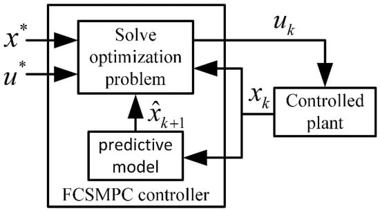
Figure 1. Structure of the single-step FCS-MPC system.

The single-step FCS-MPC algorithm can thus be formulated as the following optimization problem:

$$\underset{u_k}{\min }J({\epsilon }_k,u_k,{u_k}^{*})={{\epsilon }_k}^{T}Q{\epsilon }_k+{(u_k-{u_k}^{*})}^{T}R(u_k-{u_k}^{*})+{{\widehat{\epsilon }}_{k+1}}^{T}P{\widehat{\epsilon }}_{k+1}$$

(8)

subject to the following:

(1)

The dynamic Equation (6);

(2)

The state constraint (2) and the discrete control constraints (3).

Let the solution to the above optimization problem be denoted by $u^{opt}({\epsilon }_k,{u_k}^{*})$. Then, the closed-loop form of the FCS-MPC system can be expressed as

$${\epsilon }_{k+1}=A{\epsilon }_k+B(u^{opt}({\epsilon }_k,{u_k}^{*})-{u_k}^{*}).$$

(9)

According to Refs. [17,24], $u^{opt}({\epsilon }_k,{u_k}^{*})$ is a piecewise function. Depending on the number of candidate inputs in the control set, the number of segments can be extremely large, making direct analysis of system (9) challenging.

Given that the control input is constrained to a finite set, if the state region under investigation is bounded such that all admissible inputs selected from the control set cannot drive the system state outside the constraint set, the state constraints can be neglected. Consequently, we consider the optimal control law without state constraints, which will be derived below.

Equation (7) can be transformed into the following form:

$$J({\epsilon }_k,u_k,{u_k}^{*})={(H^{1/2}{u}_k-H^{1/2}(K{\epsilon }_k+{u_k}^{*}))}^T(H^{1/2}{u}_k-H^{1/2}(K{\epsilon }_k+{u_k}^{*}))+d({\epsilon }_k),$$

(10)

where $H=R+B^{T}PB$, $K=-H^{-1}{B}^{T}PA$ and $d(x_k)={{\epsilon }_k}^T(Q+A^{T}PA-K^{T}HK){\epsilon }_k$. The optimal control vector without state constraints can be expressed as [15,16]

$${u_k}^{of}=K{\epsilon }_k+{u_k}^{*}+H^{-1/2}w({\epsilon }_k,{u_k}^{*})$$

(11)

where $w({\epsilon }_k,{u_k}^{*})=(q_{\mathbb{V}}(H^{1/2}(K{\epsilon }_k+{u_k}^{*}))-H^{1/2}(K{\epsilon }_k+{u_k}^{*}))$, $\mathbb{V}=H^{1/2}\mathcal{U}$, $q_{\mathbb{V}}()$ denotes the Euclidean quantifier, which is defined as follows.

Definition 1 [Euclidean Vector Quantizer]. 

Consider a set $A\subseteq R^n$ and a countable (not necessarily finite) set $B\triangleq \left\{b_i\right\}\subset {\text{ℝ}}^n$, $i\in I\subseteq {\text{ℤ}}_{\ge 0}$, which satisfies that $\exists \epsilon >0:\left|b_i-b_j\right|\ge \epsilon ,\forall i,j\in I$. If function $q_B(\cdot ):A\to B$ satisfies that $q_B(a)=b_i\in B$, where $\left|a-b_i\right|\le \left|a-b_j\right|$, hold for $\forall b_j\ne b_i$; then, $q_B(\cdot )$ is a Euclidean vector quantizer.

2.3. Closed-Loop System Model in Positively Invariant Set

If there exists an invariant set of system (6) with respect to the control law (11), and this set lies within the state constraint set $\mathcal{X}$, then (11) represents the optimal solution to the optimization problem (8) within this invariant set. Consequently, the closed-loop form of system (9) can be established for further analysis. To compute this invariant set in the following discussion, the controlled system is assumed to satisfy the following condition.

Assumption 1. 

There exists a feedback control law $\tilde{K}\in {\text{ℝ}}^{m\times n}$, as well as a symmetric positive definite matrix $Q_P\in {\text{ℝ}}^{n\times n}$, such that the matrices $P$ and $R$ in the cost function (7) satisfy the following relationship:

$$P={(A+B\tilde{K})}^{T}P(A+B\tilde{K})+(Q_P+{\tilde{K}}^{T}R\tilde{K}).$$

(12)

This assumption is not overly restrictive, as it can be satisfied whenever system (1) is stabilizable.

If Assumption 1 holds, the following properties of the system matrices can be derived, which are essential in the subsequent analysis. It is straightforward to obtain

$$P-Q={(A+B\tilde{K})}^{T}P(A+B\tilde{K})+{\tilde{K}}^{T}R\tilde{K}.$$

(13)

This implies that $(P-Q)$ is positive definite, and hence

$${\lambda }_{\max }(P)-{\lambda }_{\min }(Q)>0,$$

(14)

Furthermore, similar to the derivation of (10), we have

$$A^{T}PA-P+Q-K^{T}HK=-{(\tilde{K}-K)}^{T}H(\tilde{K}-K),$$

(15)

which implies that $(A^{T}PA-P+Q-K^{T}HK)$ is negative semidefinite.

Based on (10) and (15), for the unconstrained optimal control law (11) applied to system (6), we derive

$$f{(\epsilon ,u^{of},u^{*})}^{T}Pf(\epsilon ,u^{of},u^{*})-{\epsilon }^{T}P\epsilon \le -{\epsilon }^{T}Q\epsilon -{(u^{of}-u^{*})}^{T}R(u^{of}-u^{*})+{\left|w\right|}^2$$

(16)

and therefore, the set $\Xi \triangleq \left\{\left.\epsilon \right|{\epsilon }^{T}P\epsilon \le d,d\in {\text{ℝ}}_{>0}\right\}$ is a candidate invariant set.

To determine the conditions under which $\Xi$ becomes invariant, we analyze the boundedness of $\left|w({\epsilon }_k,{u_k}^{*})\right|$ over $\Xi \times {\mathcal{U}}^{*}$. Its upper bound can be computed as follows:

(1)

Compute the set $U_h({u_k}^{*})$:

Define

$$U_h({u_k}^{*})\triangleq \left\{H^{1/2}K{\epsilon }_k+H^{1/2}{u_k}^{*}|{\epsilon }_k\in \Xi \right\}$$

(17)

Let $u_h=H^{1/2}K{\epsilon }_k+H^{1/2}{u_k}^{*}$. Since $H^{1/2}K\in {\mathbb{R}}^{m\times n}$, by augmenting it with $n-m$ linearly independent row vectors ${\tilde{k}}_1,\dots ,{\tilde{k}}_{n-m}$, we obtain a nonsingular matrix:

$${\tilde{K}}_h\triangleq \left[H^{1/2}K;{\tilde{k}}_1;\dots ;{\tilde{k}}_{n-m}\right]$$

(18)

Then, we have

$${{\tilde{U}}_h}^{*}\triangleq \left\{\left.{{\tilde{u}}_h}^{*}\right|{{\tilde{u}}_h}^{*T}{({{\tilde{K}}_h}^{-1})}^{T}P{{\tilde{K}}_h}^{-1}{{\tilde{u}}_h}^{*}\le d\right\},$$

(19)

where ${{\tilde{u}}_h}^{*}=\left[{u_h}^{*};{\tilde{u}}_1;\dots ;{\tilde{u}}_{n-m}\right]$, ${u_h}^{*}=u_h-H^{1/2}{u_k}^{*}$, and ${\tilde{u}}_1,\dots ,{\tilde{u}}_{n-m}$ are auxiliary variables to be eliminated.

Let

$${\tilde{f}}_h({{\tilde{u}}_h}^{*})\triangleq {{\tilde{u}}_h}^{*T}{({\tilde{K}}^{-1})}^{T}P{\tilde{K}}^{-1}{{\tilde{u}}_h}^{*},$$

(20)

and by setting the partial derivatives of ${\tilde{f}}_h({\tilde{u}}_h)$ with respect to the auxiliary variables to zero and solving the resulting equations, we obtain

$${\left[{\tilde{u}}_1;\dots ;{\tilde{u}}_{n-m}\right]}^T=\tilde{A}{u_h}^{*}.$$

(21)

Substituting ${{\tilde{u}}_h}^{*}=\left[I;\tilde{A}\right]{u_h}^{*}$ into the inequality ${\tilde{f}}_h({\tilde{u}}_h)\le d$ leads to

$${U_h}^{*}\triangleq \left\{\left.{u_h}^{*}\right|{u_h}^{*T}{\left[\begin{array}{c}I\\ \tilde{A}\end{array}\right]}^T{({\tilde{K}}^{-1})}^{T}P{\tilde{K}}^{-1}\left[\begin{array}{c}I\\ \tilde{A}\end{array}\right]{u_h}^{*}\le d\right\}.$$

(22)

As illustrated in Figure 2, this set is the projection of ${{\tilde{U}}_h}^{*}$ onto the $m$-dimensional hyperplane where ${u_h}^{*}$ resides.

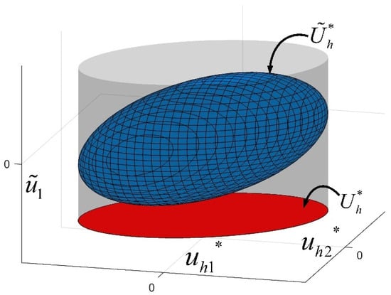
Figure 2. Illustration for relationship between ${{\tilde{U}}_h}^{*}$ and ${U_h}^{*}$ with $n=3$, $m=2$.

Thus,

$$U_h({u_k}^{*})\triangleq \left\{\left.u_h\right|{(u_h-H^{1/2}{u_k}^{*})}^T{\left[\begin{array}{c}I\\ \tilde{A}\end{array}\right]}^T{({\tilde{K}}^{-1})}^{T}P{\tilde{K}}^{-1}\left[\begin{array}{c}I\\ \tilde{A}\end{array}\right](u_h-H^{1/2}{u_k}^{*})\le d\right\}.$$

(23)

As shown in Figure 3, for each ${u_k}^{*}$, ${\mathcal{U}}_h$ is obtained by translating ${{\mathcal{U}}_h}^{*}$ in the hyperplane.

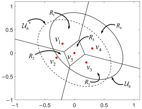
Figure 3. Illustration for relationship between $U_h$ and ${U_h}^{*}$, and the optimal space $R_i$ corresponding to each discrete control vector with $m=2$, $p=5$. The solid and dashed ellipses correspond to $U_h$ and ${U_h}^{*}$, respectively.

(2)

Calculate the upper bound of $\left|w({\epsilon }_k,{u_k}^{*})\right|$ on $\Xi \times {\mathcal{U}}^{*}$:

For each discrete control value $v_i\in H^{1/2}\mathcal{U}$, define the region [17]:

$$\begin{array}{cc}\hfill {\tilde{R}}_i& \triangleq \left\{x|{(v_i-x)}^T(v_i-x)\le {(v_j-x)}^T(v_j-x),j\ne i\right\}\hfill \\ & =\left\{x|2({v_j}^T-{v_i}^T)x\le {v_j}^T{v}_j-{v_i}^T{v}_i,j\ne i\right\}\hfill \end{array},$$

(24)

so that $q_{\mathbb{V}}(x)=v_i$ for $x\in {\tilde{R}}_i$.

Define

$$R_i({u_k}^{*})={\tilde{R}}_i\cap U_h({u_k}^{*}).$$

(25)

For each fixed ${u_k}^{*}\in {\mathcal{U}}^{*}$, solving the optimization problem

$$\underset{x\in R_i({u_k}^{*})}{\max }{f}_w(x)={(v_i-x)}^T(v_i-x)$$

(26)

over all regions $R_i({u_k}^{*})$ yields the upper bound of $\left|w({\epsilon }_k,{u_k}^{*})\right|$ over $\Xi \times {\mathcal{U}}^{*}$, denoted as

$$\Delta q\triangleq \underset{\epsilon \in \Xi ,{u_k}^{*}\in {\mathcal{U}}^{*}}{\max }\left|q_{\mathbb{V}}(H^{1/2}(K{\epsilon }_k+{u_k}^{*}))-H^{1/2}(K{\epsilon }_k+{u_k}^{*})\right|.$$

(27)

As shown in Figure 3, for each fixed ${u_k}^{*}$, (26) is a quadratic optimization problem with linear and quadratic inequality constraints, which can be solved using standard optimization tools.

Assumption 2. 

Suppose that there exists a constant $d$, such that $d>{\displaystyle \frac{\Delta q^2{\lambda }_{\max }(P)}{{\lambda }_{\min }(Q)}}$, and for all $\epsilon \in \Xi$, the corresponding state $x\in \mathcal{X}$.

If Assumption 2 holds, then from (14) and (16), for any ε ∈ Ξ ${u_k}^{*}\in {\mathcal{U}}^{*}$, we have

$$f{(\epsilon ,{\widehat{u}}^{of}(\epsilon ,u^{*}),u^{*})}^{T}Pf(\epsilon ,{\widehat{u}}^{of}(\epsilon ,u^{*}),u^{*})<d.$$

(28)

Hence, $\Xi$ is an invariant set of system (6) with respect to (11). When $x_k\in \Xi$ and ${u_k}^{*}\in {\mathcal{U}}^{*}$, the solution of (8) is

$$u^{opt}(x_k)=u^{of}(x_k)=K{\epsilon }_k+{u_k}^{*}+H^{-1/2}w({\epsilon }_k,{u_k}^{*}).$$

(29)

By treating $w({\epsilon }_k,{u_k}^{*})$ as a disturbance and denoting it as $w_k$, we have

$$w_k\in \left\{\left.x\right|\left|x\right|\le \Delta q\right\},\forall k\in {\text{ℤ}}_{\ge 0},$$

(30)

And

$$‖\mathbf{w}‖=\Delta q.$$

(31)

Thus, the closed-loop system (9) on the set $\Xi$ becomes

$${\epsilon }_{k+1}=F({\epsilon }_k,w_k)=A{\epsilon }_k+B(K{\epsilon }_k+H^{-1/2}{w}_k).$$

(32)

3. Regional ISS Theory

ISS theory is an important tool to analyze the relationship between state trajectories and inputs of nonlinear systems. This concept was first proposed in [25] and has since been extended in various directions by subsequent researchers. In practical model predictive control (MPC) applications, state and input constraints are typically present, rendering global ISS results less applicable. To address this limitation, a regional version of ISS was proposed in [26], which allows for stability analysis within a restricted domain. This concept makes it feasible to apply ISS theory to constrained MPC systems. To characterize the stability properties of the FCS-MPC system studied in this paper, we adopt the definition of regional ISS presented in [27]:

Consider a discrete-time autonomous system of the following form:

$$x_{k+1}=F(x_k,w_k),k\in {\text{ℤ}}_{\ge 0},$$

(33)

where $x_k\in {\text{ℝ}}^n$ is the state, $w_k\in {\text{ℝ}}^q$ represents an unknown disturbance, and the transition map $F(x_k,w_k)$ may be discontinuous. Given an initial state $\overline{x}$ and a disturbance sequence $\mathbf{w}$, the state trajectory of the system is denoted as $x(k,\overline{x},\mathbf{w})$.

Assumption 3. 

(1)

For system (33), the origin is an equilibrium point.

(2)

The disturbance $w_k$ satisfies $w_k\in W$  for  $\forall k\in {\text{ℤ}}_{\ge 0}$, where $W$ is a compact set containing the origin.

Definition 2 [Robust Positively Invariant Set (RPIS)]. 

Suppose that Assumption 3 holds; $\Xi \subseteq {\text{ℛ}}^n$ is an RPIS for system (33) if $F(x,w)\in \Xi$ holds for $\forall w\in W$ and $\forall x\in \Xi$.

Definition 3 [Regional Input-to-State Stability (ISS)]. 

Suppose that Assumption 3 is satisfied. Given a compact set $\Xi \subseteq {\text{ℛ}}^n$ containing the origin as an interior point, if $\Xi$ is an RPIS for system (33), and there exists a ${\mathcal{K}}_{\mathcal{L}}$-function $\beta$ and a $\mathcal{K}$-function $\gamma$ , such that

$$\left|x(k,\overline{x},w)\right|\le \beta (\left|\overline{x}\right|,k)+\gamma (‖\mathbf{w}‖),\forall k\ge 0,\forall \overline{x}\in \Xi .$$

(34)

Then the system (33) is said to be regional ISS with $\mathbf{w}\in {\text{ℳ}}_W$ in $\Xi$.

4. Analysis of System Stability and Performance

If Assumption 1 and Assumption 2 hold, then system (9) can be represented by (32) within the set $\Xi$. Moreover, system (32) satisfies Assumption 3, and $\Xi$ is an RPIS for (32). The following proof establishes the ISS property of system (32) in $\Xi$.

4.1. ISS Proof

Theorem 1. 

Suppose that Assumption 1 and Assumption 2 hold; then, system (32) is ISS in $\Xi$ with respect to the disturbance sequence $\mathbf{w}\in {\text{ℳ}}_W$.

Proof of Theorem 1. 

To facilitate the proof, we define several parameters and functions. Let $a_1={\lambda }_{\min }(P)$, $a_2={\lambda }_{\max }(P)$, $a_3={\lambda }_{\min }(Q)$, $a_4=a_3{a_2}^{-1}$, $a_5=a_2{a_3}^{-1}{b}^{-1}$,

$$V(\epsilon )\triangleq {\epsilon }^{T}P\epsilon ,$$

(35)

$$\Theta \triangleq \left\{\epsilon \left|V(\epsilon )\le a_5{‖\mathbf{w}‖}^2\right.\right\},\mathbf{w}\in {\text{ℳ}}_W,$$

(36)

where $b\in {\text{ℝ}}_{(0,1]}$. Using these definitions, the set $\Xi$ can be rewritten as

$$\Xi \triangleq \left\{\epsilon :V(\epsilon )\le d\right\}.$$

(37)

It is straightforward to obtain

$$V({\epsilon }_k)\ge a_1{\left|{\epsilon }_k\right|}^2,\forall {\epsilon }_k\in \Xi ,$$

(38)

$$V({\epsilon }_k)\le a_2{\left|{\epsilon }_k\right|}^2,\forall {\epsilon }_k\in \Xi .$$

(39)

From inequality (16), we know that

$$\Delta V({\epsilon }_k)={{\epsilon }_{k+1}}^{T}P{\epsilon }_{k+1}-{{\epsilon }_k}^{T}P{\epsilon }_k\le -a_3{\left|{\epsilon }_k\right|}^2+{\left|w_k\right|}^2,\forall {\epsilon }_k\in \Xi$$

(40)

By Assumption 2, there exists a constant $b\in {\text{ℝ}}_{(0,1]}$ such that $a_5\Delta q<d$, and thus $\Theta \subset \Xi$. If $x_k\in \Theta$, from (39), (40), and (14), we obtain

$$V({\epsilon }_{k+1})\le (1-a_4)V({\epsilon }_k)+{‖\mathbf{w}‖}^2\le a_5{‖\mathbf{w}‖}^2.$$

(41)

which implies that ${\epsilon }_{k+1}\in \Theta$. Therefore, once the state trajectory enters $\Theta$, it remains inside.

If ${\epsilon }_k\in \Xi \backslash \Theta$, from (39) and (40), it follows that there exists a constant $c>0$ such that

$$\Delta V({\epsilon }_k)\le -a_{4}V({\epsilon }_k)+{‖\mathbf{w}‖}^2\le -c.$$

(42)

As $\Xi$ is an RPIS containing the origin as an interior point for system (32), and $V(\epsilon )$ is upper bounded on $\Xi$, for any initial condition $\overline{\epsilon }\in \Xi$, there exists a finite time index

$$j_0=\min \left\{k\in {\mathbb{Z}}_{\ge 0}:\epsilon (k,\overline{\epsilon },w)\in \Theta \right\}$$

(43)

For $k<j_0$, we must have $V(\epsilon (k,\overline{\epsilon },\mathbf{w}))>a_5{‖\mathbf{w}‖}^2$. From (39) and (40), it follows that

$$V(\epsilon (k,\overline{\epsilon },\mathbf{w}))\le (1-(1-b)a_4)V(\epsilon (k-1,\overline{\epsilon },\mathbf{w})),$$

(44)

and iteratively

$$V(\epsilon (k,\overline{\epsilon },\mathbf{w}))\le {(1-(1-b)a_4)}^{k}V(\overline{\epsilon }).$$

(45)

Thus, we have

$$V(\epsilon (k,\overline{\epsilon },\mathbf{w}))\le \max \left\{{\beta }_a(V(\overline{\epsilon }),k),a_5{‖\mathbf{w}‖}^2\right\},\overline{\epsilon }\in \Xi ,k\in {\text{ℤ}}_{\ge 0},$$

(46)

where ${\beta }_a(\epsilon ,r)={(1-(1-b)a_4)}^r\epsilon$, which is a ${\mathcal{K}}_{\mathcal{L}}$-function.

From inequality (38), it follows that

$$\left|\epsilon (k,\overline{\epsilon },\mathbf{w})\right|\le \max \left\{\sqrt{{a_1}^{-1}{\beta }_a(a_2{\left|\overline{\epsilon }\right|}^2,k)},\sqrt{{a_1}^{-1}{a}_5{‖\mathbf{w}‖}^2}\right\},\overline{\epsilon }\in \Xi ,k\in {\text{ℤ}}_{\ge 0}.$$

(47)

Finally, define

$$\beta (\epsilon ,r)=\sqrt{{a_1}^{-1}{\beta }_a(a_2{\left|\epsilon \right|}^2,r)},$$

(48)

$$\gamma (\epsilon )\triangleq \sqrt{{a_1}^{-1}{a}_5{\epsilon }^2}.$$

(49)

It can be verified that $\beta (\epsilon ,s)$ is a ${\mathcal{K}}_{\mathcal{L}}$-function and $\gamma (\epsilon )$ is a $\mathcal{K}$-function. Therefore, the system (32) is ISS in $\Xi$ with respect to the disturbance sequence $\mathbf{w}\in {\text{ℳ}}_W$. □

4.2. Performance Estimation

This section presents a computational procedure for estimating the domain of attraction and the ultimate bounded region of the system state trajectories, based on the results established in Section 2.3 and Section 4.1. In Section 5.1, the proposed method will be illustrated through simulation examples, where we demonstrate the relationship between the domain of attraction and system stability, as well as between the ultimate bounded region and steady-state performance.

According to inequality (46), the state trajectories originating from $\Xi$ will asymptotically approach and eventually enter the set $\Theta$. Specifically, we have

$$\underset{k\to \infty }{\lim }\epsilon {(k,\overline{\epsilon },\mathbf{w})}^{T}P\epsilon (k,\overline{\epsilon },\mathbf{w})\le a_5\Delta q^2,\forall \overline{x}\in \Xi .$$

(50)

Once the state trajectory enters $\Theta$, the feasible set of optimal control values changes, leading to a corresponding update in $\Delta q$. If the new value of $\Delta q$ recalculated over $\Theta$ still satisfies Assumption 2, then ISS analysis can be iteratively applied on the newly defined region $\Theta$. This process can continue until Assumption 2 is no longer satisfied.

Based on this idea, the following iterative algorithm (Algorithm 1) is proposed for estimating the domain of attraction and the ultimate bounded region of system (9):

Algorithm 1 Calculation of Domain of Attraction and Ultimate Bounded Region
1:	Input the parameters $d$$,a_4$ and the number of iterations $n$. Let $d_{MPC}=d$.
2:	Extend $H^{1/2}K\in {\text{ℝ}}^{m\times n}$ $\mathrm{to}\mathrm{obtain}{\tilde{K}}_h\in {\text{ℝ}}^{n\times n}$.
3:	Set the partial derivative of Equation (20) with respect to the auxiliary control vari-
4:	able to zero, and solve the system of equations to obtain Equation (21).
5:	Obtain $U_h({u_k}^{*})$ according to Equation (23).
6:	for i = 1: n
7:	For each ${u_k}^{*}$ in ${\mathcal{U}}^{*}$, $\mathrm{partition}{U}_h({u_k}^{*})$ $\mathrm{into}{R}_i({u_k}^{*})$ according to (25).
8:	Use the optimization tool to calculate the maximum value of $\left|w({\epsilon }_k,{u_k}^{*})\right|$ on
9:	all $R_i({u_k}^{*})$$\mathrm{and}\mathrm{record}\mathrm{it}\mathrm{in}\Delta q$.
10:	if $d>{a_4}^{-1}\Delta q$
11:	$d={a_4}^{-1}\Delta q$
12:	else
13:	Record the value of $d$ that last satisfies $d>{a_4}^{-1}\Delta q$ $\mathrm{as}{d}_f$.
14:	Break the loop.
15:	end if
16:	end for
17:
18:	if i = 1
19:	The system is unstable on ${\mathcal{X}}_{MPC}$.
20:	else
21:	The system is stable on  ${\mathcal{X}}_{MPC}$ and ultimately converges to ${\Theta }_f$.
22:	end if

Then, the domain of attraction and the ultimate bounded region of system (9) can be expressed as

$${\mathcal{X}}_{MPC}=\left\{\left.\epsilon \right|{\epsilon }^{T}P\epsilon \le d_{MPC}\right\},$$

(51)

$${\Theta }_f=\left\{\left.\epsilon \right|{\epsilon }^{T}P\epsilon \le d_f\right\}.$$

(52)

Remark 1. 

The number of iterations $n$ is introduced to limit the computational time. By setting a maximum number of iterations within an acceptable range, a more accurate estimate of the ultimate bounded region ${\Theta }_f$ can be obtained without excessive computational burden.

Remark 2. 

According to [28], it is generally permissible for the state to temporarily exceed the constraint limits. This is because, as long as ${\Theta }_f$ is within the state constraint bounds, the state trajectory will quickly converge back within the state constraints.

5. Simulation Experiment

Two models are considered in this section. The first is an open-loop unstable mathematical model with a fixed reference value, and the second is a three-phase inverter simulation model with a periodic reference signal. In both cases, the controller parameters are designed based on the procedures described in the previous sections. The stability and performance of the system are then analyzed, and the accuracy of the theoretical analysis is verified through simulations.

5.1. Illustrative Mathematical Example

The plant model is defined as

$$A=\left[\begin{array}{cc}0.2& 0\\ 0.2& 1.1\end{array}\right],B=\left[\begin{array}{cc}0.3& 0.4\\ 0.5& 0.2\end{array}\right];$$

The state constraint set and the finite control set are

$$\mathcal{X}=\left\{x:{\left[\begin{array}{cccc}1& -1& 0& 0\\ 0& 0& 1& -1\end{array}\right]}^{T}x\le {\left[\begin{array}{cccc}3.8& -0.2& 3.2& -0.4\end{array}\right]}^T\right\},$$

(53)

$$\mathcal{U}=\left\{\left[\begin{array}{c}-3.6361\\ 7.0134\end{array}\right],\left[\begin{array}{c}-4.3848\\ 7.3378\end{array}\right],\left[\begin{array}{c}-3.5010\\ 6.5765\end{array}\right],\left[\begin{array}{c}-4.2496\\ 6.9009\end{array}\right]\right\},$$

(54)

The weighting matrices are

$$Q=\left[\begin{array}{cc}1& 0\\ 0& 1\end{array}\right],R=\left[\begin{array}{cc}0.1& 0\\ 0& 0.1\end{array}\right],P=\left[\begin{array}{cc}1.0138& 0.0374\\ 0.0374& 1.5926\end{array}\right],$$

where $P$ is obtained by solving the discrete Riccati equation. The reference state is $x^{*}={\left[\begin{array}{cc}2& 1.8\end{array}\right]}^T$, and the corresponding steady-state control is $u^{*}={\left[\begin{array}{cc}-3.9429& 6.9571\end{array}\right]}^T$.

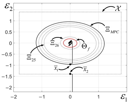
Using Algorithm 1, the domain of attraction and ultimate bounded region are calculated as shown in Figure 4.

Figure 4. Calculation results of the system’s domain of attraction and convergence region, and the state error trajectories. ${\epsilon }_1$, ${\epsilon }_2$ represent the two components of the error vector $\epsilon$. The black solid circle represents the domain of attraction, and the red circle indicates the convergence region. The black dashed circles illustrate the intermediate iterations in Algorithm 1, and the black dashed box denotes the imposed state constraints.

$${\Xi }_{MPC}=\left\{\left.\epsilon \right|{\epsilon }^{T}P\epsilon \le 1.47\right\},$$

(55)

and after 30 iterations, the estimated ultimate bounded region becomes

$${\Theta }_f=\left\{\left.\epsilon \right|{\epsilon }^{T}P\epsilon \le 0.0585\right\}.$$

(56)

From the discussion in Section 4.1, it can be concluded that the domain of attraction represents the region within which the system stability is guaranteed. If the initial state error belongs to ${\Xi }_{MPC}$, the error trajectory will converge to ${\Theta }_f$ and remain within ${\Xi }_{MPC}$ in this process. Otherwise, it may diverge.

For example, with initial error ${\overline{x}}_1={\left[\begin{array}{cc}2& 0.8393\end{array}\right]}^T$, the trajectory converges to ${\Theta }_f$. However, for ${\overline{x}}_2={\left[\begin{array}{cc}2& 0.41\end{array}\right]}^T$, the system diverges, as shown in Figure 4 and Figure 5, verifying the regional ISS property.

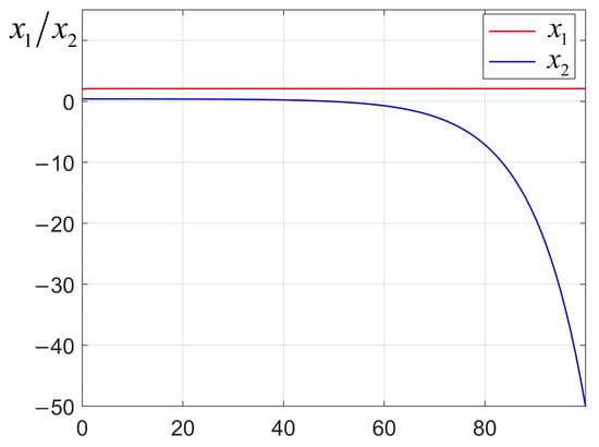
Figure 5. System state trajectories starting from ${\overline{x}}_2={\left[\begin{array}{cc}2& 0.41\end{array}\right]}^T$.

According to the definition of ${\Theta }_f$, the Euclidean norm of the steady-state error satisfies

$$\underset{k\to \infty }{\lim }\left|\epsilon (k,\overline{\epsilon },\mathbf{w})\right|\le \sqrt{d_f/{\lambda }_{\min }(P)}=0.2405.$$

(57)

Therefore, the size of ultimate bounded region represents the steady-state error of the system. The norm of the state error starting from ${\overline{x}}_1$ is shown in Figure 6. As shown in Figure 6, this bound aligns with simulation results. The state waveform is illustrated in Figure 7.

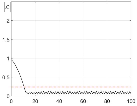
Figure 6. Estimated performance results and norm of state error starting from ${\overline{x}}_1$. The black solid line represents the Euclidean norm of the state error trajectory starting from ${\overline{x}}_1$, and the red dashed line indicates the estimated upper bound of the steady-state error norm.

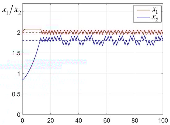
Figure 7. System state waveform starting from ${\overline{x}}_1$. The red and blue dashed lines indicate the reference values of $x_1$ and $x_2$.

5.2. Two-Level Inverter Simulation Model

The circuit is shown in Figure 8, with parameters $V_{dc}=80 \mathrm{V}$, $r=5 \mathrm{\Omega }$ and $L=17 \mathrm{mH}$.

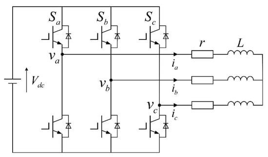
Figure 8. Two-level inverter topology. The arrows indicate the reference directions of phase currents $i_a$, $i_b$ and $i_c$.

In the two-phase rotating coordinate system, the continuous-time model is

$${\left[\begin{array}{cc}{\displaystyle \frac{d{i}_{\alpha }}{dt}}& {\displaystyle \frac{d{i}_{\beta }}{dt}}\end{array}\right]}^T=A_c{\left[\begin{array}{cc}{i}_{\alpha }& i_{\beta }\end{array}\right]}^T+B_c{\left[\begin{array}{cc}{u}_{\alpha }& u_{\beta }\end{array}\right]}^T,$$

(58)

where

$$A_c=\left[\begin{array}{cc}-{\displaystyle \frac{r}{L}}& 0\\ 0& -{\displaystyle \frac{r}{L}}\end{array}\right],B_c=\left[\begin{array}{cc}{\displaystyle \frac{1}{L}}& 0\\ 0& {\displaystyle \frac{1}{L}}\end{array}\right].$$

Using zero-order hold with sampling time $T=75 \mathrm{\mu }s$, we discretize the system

$$A=e^{A_{c}T},$$

(59)

$$B=(e^{A_{c}T}-I){A_c}^{-1}{B}_c.$$

(60)

Based on the circuit structure, the finite control set can be represented as

$$\mathcal{U}=U_{dc}\left\{\left[\begin{array}{c}0\\ 0\end{array}\right],\left[\begin{array}{c}-1/3\\ -1/\sqrt{3}\end{array}\right],\left[\begin{array}{c}-1/3\\ 1/\sqrt{3}\end{array}\right],\left[\begin{array}{c}-2/3\\ 0\end{array}\right],\left[\begin{array}{c}2/3\\ 0\end{array}\right],\left[\begin{array}{c}1/3\\ -1/\sqrt{3}\end{array}\right],\left[\begin{array}{c}1/3\\ 1/\sqrt{3}\end{array}\right],\left[\begin{array}{c}0\\ 0\end{array}\right]\right\}.$$

(61)

To simplify analysis, the state constraints are rewritten in terms of error

$$\mathcal{X}=\left\{x\left|{\left[\begin{array}{cccc}1& -1& 0& 0\\ 0& 0& 1& -1\end{array}\right]}^T\epsilon \le {\left[\begin{array}{cccc}5.5& 5.5& 5.5& 5.5\end{array}\right]}^T\right.\right\},$$

(62)

which indicates that the state variables do not exceed a certain range from the reference value.

The cost matrices are

$$Q=\left[\begin{array}{cc}1& 0\\ 0& 1\end{array}\right],R=\left[\begin{array}{cc}0.001& 0\\ 0& 0.001\end{array}\right],P=\left[\begin{array}{cc}5.1165& 0\\ 0& 5.1165\end{array}\right]$$

where $P$ is obtained by solving the discrete Riccati equation. The reference is ${x_k}^{*}={\left[\begin{array}{cc}5\cos (100\pi kT)& 5\sin (100\pi kT)\end{array}\right]}^T$, and the steady-state control is ${u_k}^{*}=B^{-1}({x_{k+1}}^{*}-A{x_k}^{*})$.

Using Algorithm 1, as shown in Figure 9, we obtain the following:

$${\Xi }_{MPC}=\left\{\left.\epsilon \right|{\epsilon }^{T}P\epsilon \le 64.2328\right\}.$$

(63)

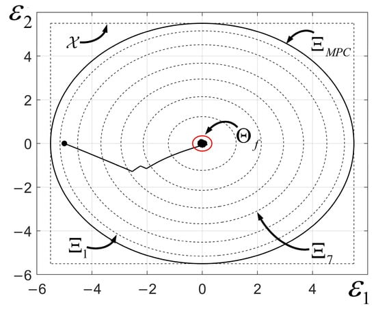
Figure 9. Calculation results of the system’s domain of attraction and convergence region, and the state error trajectories. ${\epsilon }_1$, ${\epsilon }_2$ represent the two components of the error vector $\epsilon$. The black solid circle represents the domain of attraction, and the red circle indicates the convergence region. The black dashed circles illustrate the intermediate iterations in Algorithm 1, and the black dashed box denotes the imposed state constraints.

After iterations,

$${\Theta }_f=\left\{\left.\epsilon \right|{\epsilon }^{T}P\epsilon \le 0.263\right\}.$$

(64)

For initial value $\overline{x}={\left[\begin{array}{cc}0& 0\end{array}\right]}^T$, the error state trajectory, as shown in Figure 9, converges to ${\Theta }_f$.

According to the definition of ${\Theta }_f$, the Euclidean norm of the steady-state error satisfies

$$\underset{k\to \infty }{\lim }\left|\epsilon (k,\overline{\epsilon },\mathbf{w})\right|\le 0.3520.$$

(65)

as shown in Figure 10, aligning with the performance estimation results. Additionally, the state waveform is illustrated in Figure 11.

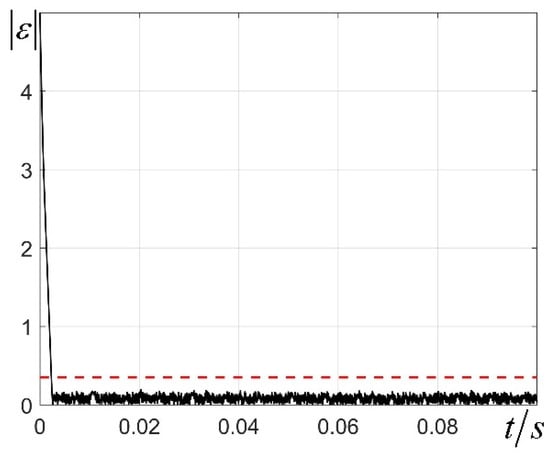
Figure 10. Estimated performance results and norm of state error starting from $\overline{x}$. The black solid line represents the Euclidean norm of the state error trajectory starting from $\overline{x}$, and the red dashed line indicates the estimated upper bound of the steady-state error norm.

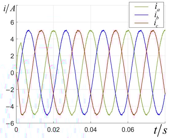
Figure 11. System state trajectories starting from $\overline{x}$.

Through the analysis of the mathematical model and circuit model, the specific calculation process of Algorithm 1 is elucidated, and the relationship between the domain of attraction and system stability, as well as the relationship between the ultimate bounded region and steady-state performance of the system, is shown. Additionally, the results of the analysis have been validated, proving the effectiveness of the analysis method and its applicability to a class of power electronic converters.

6. Conclusions

In this paper, we first conducted a detailed analysis of the closed-loop model of the single-step FCS-MPC system. Based on the relevant concepts of regional input-to-state stability (ISS) theory, we derived sufficient conditions to ensure the regional ISS of the system, established the relationship between quantization error and system performance, and provided a complete theoretical derivation and proof. On this basis, an iterative algorithm was proposed for estimating the system’s domain of attraction and ultimate bounded region. Finally, simulation experiments were carried out to verify the correctness of the theoretical analysis, which also demonstrated the relationship between the domain of attraction and system stability, as well as between the ultimate bounded region and steady-state performance. The results indicate that appropriate parameter design can provide stability assurance for the system, and the proposed method enables an intuitive illustration of the stability characteristics and steady-state performance under different parameter settings, thereby offering theoretical guidance for the design of a class of FCS-MPC systems. Compared with existing studies, this paper presents a more general quantization error calculation method, which extends the analysis from previously studied single-input systems to multi-input systems with state constraints. Furthermore, we provide a complete derivation of the sufficient conditions for ISS under certain conditions, thereby addressing the incomplete theoretical proofs observed in some earlier works within the same analytical framework. In addition, the iterative algorithm proposed in this study serves as an effective tool for exploring the relationship between system parameters and performance, filling a gap in the current research within this framework.

References

- Rodriguez, J.; Garcia, C.; Mora, A.; Flores-Bahamonde, F.; Acuna, P.; Novak, M.; Zhang, Y.; Tarisciotti, L.; Davari, S.A.; Zhang, Z.; et al. Latest Advances of Model Predictive Control in Electrical Drives—Part I: Basic Concepts and Advanced Strategies. IEEE Trans. Power Electron. 2022, 37, 3927–3942. [Google Scholar] [CrossRef]
- Rodriguez, J.; Garcia, C.; Mora, A.; Davari, S.A.; Rodas, J.; Valencia, D.F.; Elmorshedy, M.; Wang, F.; Zuo, K.; Tarisciotti, L.; et al. Latest Advances of Model Predictive Control in Electrical Drives—Part II: Applications and Benchmarking with Classical Control Methods. IEEE Trans. Power Electron. 2022, 37, 5047–5061. [Google Scholar] [CrossRef]
- Karamanakos, P.; Geyer, T. Guidelines for the Design of Finite Control Set Model Predictive Controllers. IEEE Trans. Power Electron. 2020, 35, 7434–7450. [Google Scholar] [CrossRef]
- Gulbudak, O.; Gokdag, M. Finite Control Set Model Predictive Control Approach of Nine Switch Inverter-Based Drive Systems: Design, Analysis, and Validation. ISA Trans. 2021, 110, 283–304. [Google Scholar] [CrossRef] [PubMed]
- Saberi, S.; Rezaie, B. Robust Adaptive Direct Speed Control of PMSG-Based Airborne Wind Energy System Using FCS-MPC Method. ISA Trans. 2022, 131, 43–60. [Google Scholar] [CrossRef] [PubMed]
- Wu, W.; Wang, D.; Peng, Z.; Liu, X. Model Predictive Direct Power Control for Modular Multilevel Converter under Unbalanced Conditions with Power Compensation and Circulating Current Reduction. ISA Trans. 2020, 106, 318–329. [Google Scholar] [CrossRef]
- Ayala, M.; Doval-Gandoy, J.; Rodas, J.; Gonzalez, O.; Gregor, R. Current Control Designed with Model Based Predictive Control for Six-Phase Motor Drives. ISA Trans. 2020, 98, 496–504. [Google Scholar] [CrossRef]
- Vazquez, S.; Rodriguez, J.; Rivera, M.; Franquelo, L.G.; Norambuena, M. Model Predictive Control for Power Converters and Drives: Advances and Trends. IEEE Trans. Ind. Electron. 2017, 64, 935–947. [Google Scholar] [CrossRef]
- Quevedo, D.E.; Aguilera, R.P.; Geyer, T. Predictive Control in Power Electronics and Drives: Basic Concepts, Theory, and Methods. In Advanced and Intelligent Control in Power Electronics and Drives; Orłowska-Kowalska, T., Blaabjerg, F., Rodríguez, J., Eds.; Springer International Publishing: Cham, Switzerland, 2014; pp. 181–226. ISBN 978-3-319-03401-0. [Google Scholar] [CrossRef]
- Karamanakos, P.; Liegmann, E.; Geyer, T.; Kennel, R. Model Predictive Control of Power Electronic Systems: Methods, Results, and Challenges. IEEE Open J. Ind. Appl. 2020, 1, 95–114. [Google Scholar] [CrossRef]
- Akter, M.P.; Mekhilef, S.; Mei Lin Tan, N.; Akagi, H. Modified Model Predictive Control of a Bidirectional AC–DC Converter Based on Lyapunov Function for Energy Storage Systems. IEEE Trans. Ind. Electron. 2016, 63, 704–715. [Google Scholar] [CrossRef]
- Makhamreh, H.; Trabelsi, M.; Kükrer, O.; Abu-Rub, H. A Lyapunov-Based Model Predictive Control Design with Reduced Sensors for a PUC7 Rectifier. IEEE Trans. Ind. Electron. 2021, 68, 1139–1147. [Google Scholar] [CrossRef]
- Komurcugil, H.; Guler, N.; Bayhan, S. Weighting Factor Free Lyapunov-Function-Based Model Predictive Control Strategy for Single-Phase T-Type Rectifiers. In Proceedings of the IECON 2020 The 46th Annual Conference of the IEEE Industrial Electronics Society, Singapore, 18–21 October 2020; pp. 4200–4205. [Google Scholar] [CrossRef]
- Guler, N.; Komurcugil, H. Energy Function Based Finite Control Set Predictive Control Strategy for Single-Phase Split Source Inverters. IEEE Trans. Ind. Electron. 2022, 69, 5669–5679. [Google Scholar] [CrossRef]
- Quevedo, D.E.; Doná, J.A.D.; Goodwin, G.C. RECEDING HORIZON LINEAR QUADRATIC CONTROL WITH FINITE INPUT CONSTRAINT SETS. IFAC Proc. Vol. 2002, 35, 183–188. [Google Scholar] [CrossRef]
- Quevedo, D.E.; De Dona, J.A.; Goodwin, G.C. On the Dynamics of Receding Horizon Linear Quadratic Finite Alphabet Control Loops. In Proceedings of the 41st IEEE Conference on Decision and Control, 2002, Las Vegas, NV, USA, 10–13 December 2002; Volume 3, pp. 2929–2934. [Google Scholar] [CrossRef]
- Quevedo, D.E.; Goodwin, G.C.; De Doná, J.A. Finite Constraint Set Receding Horizon Quadratic Control. Int. J. Robust Nonlinear Control 2004, 14, 355–377. [Google Scholar] [CrossRef]
- Aguilera, R.P.; Quevedo, D.E. On the Stability of MPC with a Finite Input Alphabet. IFAC Proc. Vol. 2011, 44, 7975–7980. [Google Scholar] [CrossRef]
- Aguilera, R.P.; Quevedo, D.E. Stability Analysis of Quadratic MPC with a Discrete Input Alphabet. IEEE Trans. Autom. Control 2013, 58, 3190–3196. [Google Scholar] [CrossRef]
- Aguilera, R.P.; Quevedo, D.E. Predictive Control of Power Converters: Designs with Guaranteed Performance. IEEE Trans. Ind. Inform. 2015, 11, 53–63. [Google Scholar] [CrossRef]
- Xu, D.; Lazar, M. Finite Control Set Model Predictive Control with Limit Cycle Stability Guarantees. arXiv 2024, arXiv:2407.07615. Available online: http://arxiv.org/abs/2407.07615 (accessed on 22 April 2025).
- Xu, D.; Damsma, S.; Lazar, M. On the Steady-State Behavior of Finite-Control-Set MPC with an Application to High-Precision Power Amplifiers. In Proceedings of the 2022 European Control Conference (ECC), London, UK, 12–15 July 2022; pp. 820–825. Available online: https://ieeexplore.ieee.org/abstract/document/9838191 (accessed on 22 April 2025).
- Egidio, L.N.; Daiha, H.R.; Deaecto, G.S. Global Asymptotic Stability of Limit Cycle and H2/H∞ Performance of Discrete-Time Switched Affine Systems. Automatica 2020, 116, 108927. [Google Scholar] [CrossRef]
- Bemporad, A.; Morari, M.; Dua, V.; Pistikopoulos, E.N. The Explicit Linear Quadratic Regulator for Constrained Systems. Automatica 2002, 38, 3–20. [Google Scholar] [CrossRef]
- Sontag, E.D. Smooth Stabilization Implies Coprime Factorization. IEEE Trans. Autom. Control 1989, 34, 435–443. [Google Scholar] [CrossRef]
- Nesic, D.; Laila, D.S. A Note on Input-to-State Stabilization for Nonlinear Sampled-Data Systems. IEEE Trans. Autom. Control 2002, 47, 1153–1158. [Google Scholar] [CrossRef]
- Raimondo, D.M. Nonlinear Model Predictive Control: Stability, Robustness and Applications. Ph.D. Thesis, Università degli Studi di Pavia, Pavia, Italy, 2009. Available online: http://sisdin.unipv.it/labsisdin/raimondo/publications.php (accessed on 18 February 2025).
- Preindl, M. Robust Control Invariant Sets and Lyapunov-Based MPC for IPM Synchronous Motor Drives. IEEE Trans. Ind. Electron. 2016, 63, 3925–3933. [Google Scholar] [CrossRef]
Disclaimer/Publisher’s Note: The statements, opinions and data contained in all publications are solely those of the individual author(s) and contributor(s) and not of MDPI and/or the editor(s). MDPI and/or the editor(s) disclaim responsibility for any injury to people or property resulting from any ideas, methods, instructions or products referred to in the content. |
© 2025 by the authors. Licensee MDPI, Basel, Switzerland. This article is an open access article distributed under the terms and conditions of the Creative Commons Attribution (CC BY) license (https://creativecommons.org/licenses/by/4.0/).