The
i-th attribute sequence of length
for the defined historical time period is shown in Equation (
2), the attribute sequence of length
is shown in Equation (
3), and the sequence of the power load data is shown in Equation (
4):
where
denotes the attribute data, and the sequence of attributes and the sequence of power load data comprises the power load sequence as
, and
is the power load data.
3.3.1. Multiple Timescale Segmentation
Since the power load data change periodically and show different trends in different time periods, there are certain shortcomings in using standard time models such as LSTM and GRU for feature extraction [
38]. These standard time models typically operate on a single timescale. Long time steps are required to capture long-term trends, which makes it easy to ignore short-term local details, and it is difficult to balance short-term local patterns and long-term trends. Moreover, the gating mechanism of these models is rather complex, leading to higher training costs.
Multi-time scale analysis can extract features at multiple resolutions, allowing the model to learn data at multiple levels, enhancing the accuracy and robustness of the prediction, and improving the overall performance of the model [
39]. Therefore, this study obtains different scale data through multi-timescale segmentation, learns feature representations at different scales and abstraction levels, and captures the short-term and long-term dependencies of time series. Specifically, by setting sliding windows with different lengths and step sizes, the original time series is sampled at multiple scales, which further enhances the comprehensive performance ability of short-term prediction and long-term trend judgment of the model [
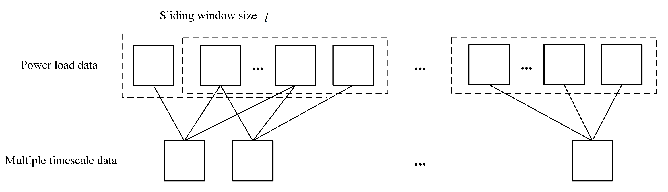
40]. The multi-timescale segmentation method proposed in this paper is shown in
Figure 3.
As can be seen from
Figure 3, the multiple timescale segmentation uses a sliding window to obtain the power load data for consecutive time periods, and the power load data within the window is averaged to obtain the multi-timescale data, which is calculated as shown in Equation (
5):
where
is the power load data,
l is the window size, and
l is the multi-timescale data obtained from the segmentation; the specific formula for multi-timescale data segmentation of
is shown in Equation (
6):
where
is the multiple timescale segmentation.
In this paper, two multi-timescale segmentation results are obtained, namely, medium timescale and high timescale. The window size
l in the medium timescale stage is 4, and the window size
l in the high timescale stage is 7. The medium timescale sequence of length
n is shown in Equation (
7):
where
is the medium timescale sequence. The high timescale sequence of length
n is shown in Equation (
8):
In Equation (
8),
is the the high timescale sequence. Then, the multi-timescale segmentation of the power load data is carried out through the moving average method, as shown in Equation (
9):
where
is the power load sequence obtained after multi-timescale segmentation.
The power load sequence is embedded as the input. At the encoder side, the input is a power load sequence of length n from the historical time period . At the decoder side, the input is a power load sequence of length from the historical time period .
3.3.2. Input Embedding
For the input embedding [
41] of
, the location and time information of the power load is obtained by fusion time localization encoding during the input embedding process. The fusion time localization encoding contains local position encoding and global time encoding to obtain the local position and global time information of the power load data, respectively. Local position encoding is used to help the model extract the relative positions between the power load data; the specific equations of local position coding for
are shown in Equations (
10) and (
11):
where
denotes the vector dimension,
j denotes the dimension of the vector dimension, the local positional encoding uses
for even dimensions and
for odd dimensions, and the coded information of all the dimensions of
makes up the local position coding of
. The local position coding is relative position information which helps the model to extract local dependencies, but it is not possible to obtain the temporal information of the power load data to extract temporal correlations, so the global time encoding proposed in Informer [
42] is introduced.
Global time encoding considers the actual time information of the power load data, and for the time corresponding to the power load data , extracts its exact time information. Assuming that the time corresponding to the power load data is “26 December 2017 11:30”, the number of days in the year before 26 December 2017, the number of days in the month before the 26 December, the number of days in the week before which the 26th is located, 11:00 and 30:00 are all extracted from the vector representation, and the vector representation is [359, 25, 1, 11, 30].
The power load data values, local position encoding and global time encoding in the power load sequence
are converted into a vector fusion of dimension
to be embedded into the encoder as shown in Equation (
12):
where
is the embedding value of the power load sequence
,
is the local position encoded embedding of the power load sequence
,
is the global time encoded embedding of the power load sequence
, and
is the input embedding result of the power load sequence
.
3.3.3. Encoder
(1) Multi-head attention mechanism
The results of the input embedding are fed to the encoder, which first performs the attention computation by means of the multi-head attention mechanism [
43]. The dimension for
, query
Q, and key
K, and the dimension for
value
V provide input to the attention mechanism. The dot product of the query and all keys is computed, dividing by
for scaling, obtaining the weights of the values through the function, and multiplying by
V, as shown in Equation (
13).
The multi-head attention mechanism projects the query
Q, the key
K, and the value
V multiple times to
, and the
and
dimensions, with different learned linear projections, respectively, where the number of heads is
h,
, and
calculated as in Equation (
14):
At each projection level of query, key, and value, the attention function is executed in parallel to generate
dimensional output values, which are concatenated and projected again to obtain the final value. The specific formula for joining different levels of attention and projecting them again is shown in Equation (
15):
where
,
,
and
are the learning parameters of the
ith head,
is the connection,
is the learnable parameter in the projection of the connection, and
is the computation of the multi-head attention.
(2) Residuals and layer normalization
After completing the computation of the multiple attention, residual and layer normalization [
44] is carried out. To achieve the residual, the input and output of the previous layer are summed. Then, layer normalization is performed on the residual results. The specific formula for residual and layer normalization is shown in Equation (
16),
where
is the input of the layer before residual and layer normalization,
is the output of the layer before residual and layer normalization,
denotes layer normalization, and
is the output of the completed attention computation with residual and layer normalization.
(3) Depthwise separable convolutional block
Convolutional neural networks have efficient feature extraction ability and can be used for power load time series feature extraction [
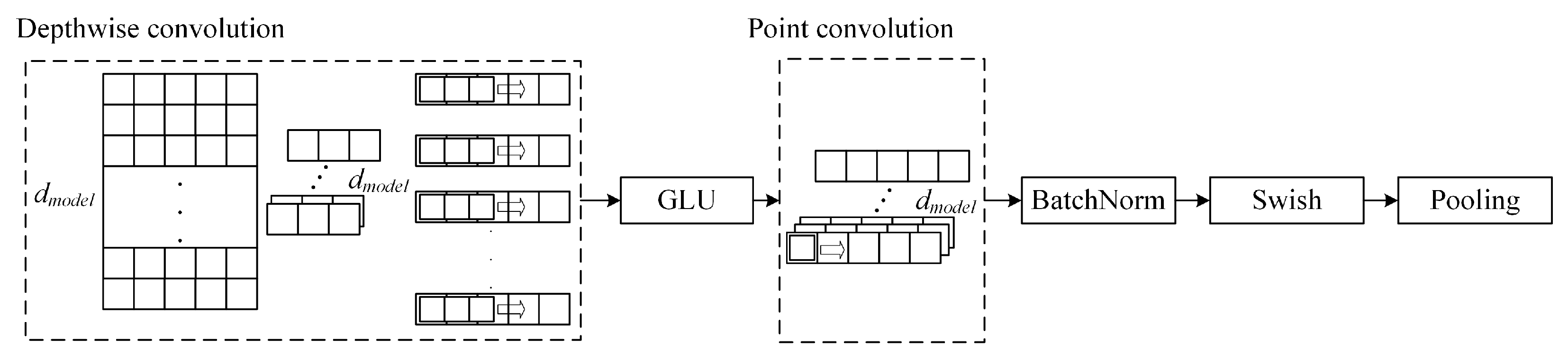
45]. Depthwise separable convolution is a kind of convolutional neural network, containing a depthwise convolutional layer for depth extraction and a pointwise convolutional layer for point extraction, which can be extracted in the direction of the channel and the point of the power load time series features. Deep convolution performs convolution operations on each input channel separately and is able to effectively capture local temporal dependencies. Pointwise convolutions (1 × 1 convolutions) perform feature mixing on the channel dimension and are able to fuse features from different channels to capture more complex feature combinations.
In this paper, we construct a convolutional block containing depthwise separable convolution, which mainly contains depthwise convolution, GLU activation, pointwise convolution, BatchNorm, Swish activation, and pooling, and the structure of the depthwise separable convolutional block is shown in
Figure 4.
As can be seen from
Figure 4, in the depthwise separable convolution block, the deep features are first extracted through the depthwise convolution in the channel direction by the convolution operation; that is, each dimension of the data is convolved separately, and its specific formula is shown in Equation (
17):
where
is the output after attention computation and residual and layer normalization,
is the transposition of
,
is the channel-by-channel convolution computation, and
is the output after depthwise convolution.
The activation is performed with the
function, which has a gate mechanism that helps the network to better capture long-term dependencies in the sequence data; the specific formula for the
function is shown in Equation (
18):
where
is the input,
and
are the two parts of
split evenly,
represents the sigmoid activation of
B, ⨂ is the Hadamard product operation, and
is the output of GLU activation.
After the deep features are extracted and activated, a one-dimensional convolution with a convolution kernel size of 1 is used to perform a point-by-point operation in the point direction, which is given by Equation (
19):
In Equation (
19),
is the output after point-by-point convolution, and the
means pointwise convolution on
.
Using BatchNorm to normalize
to avoid gradient explosion, BatchNorm is normalized on a batch basis. Taking
in one of the batches as an example, the specific formula of BatchNorm normalized on
is shown in Equation (
20):
where
is the batch mean,
is the standard deviation,
is the value that avoids 0 in the denominator,
and
are the affine change indices, and the output after BatchNorm is
.
The
activation is used for gradient smoothing to avoid jumping output values. The function of
activation is shown in Equation (
30):
In Equation (
30),
is the output of
after Swish activation. Finally, the pooling layer is used to compress the extracted features and generate more important feature information to improve the generalization ability, and the depthwise separable convolutional block output
.
Assume that in the power load data, the sequence length is
T, the number of input channels is
, the number of output channels is
, and the convolution kernel size is
K. In time-series feature extraction, the time complexity of standard convolution is represented in Equation (
22):
where
is the complexity of the traditional convolution. Each convolution operation requires traversing both the kernel size
K and sequence length
T.
The time complexity of depthwise convolution and pointwise convolution is calculated in the following way:
where
is the complexity of the depthwise convolution,
is the complexity of the pointwise convolution. The total time complexity of depthwise separable convolution is represented in Equation (
25):
where
is the total time complexity of the depthwise separable convolution. When
C and
K are large, the time complexity of traditional convolution is significantly higher than that of depth-separable convolution. Therefore, depthwise separable convolution has obvious advantages in time efficiency, which can reduce the computational load and accelerate the training and inference speed of the model.
(4) Feed-forward network
Each encoder and decoder contains a fully connected feed-forward network, which consists of two linear transformations with different parameters and a
activation in the middle [
46]. The specific formula for the output of the depthwise separable convolutional block to be computed by the feed-forward network is shown in Equation (
26):
where
is the output of the depthwise separable convolutional block,
and
are the weights of the feed-forward network, and
and
are the biases.


