Abstract
Understanding how past factors influence ion channel kinetics is essential for understanding complex phenomena in cardiac electrophysiology, such as early afterdepolarizations (EADs), which are abnormal depolarizations during the action potential plateau associated with life-threatening arrhythmias. We developed a mathematical framework that extends Hodgkin-Huxley type equations with gamma Mittag-Leffler distributed delays, using tools from Fractional Calculus. Traditional memoryless two-variable models fail to reproduce EADs. Our approach modifies FitzHugh-Nagumo, Mitchell-Schaeffer, and Karma cardiac models, enabling the generation of EADs in each of them. We analyze the emergence of these oscillations by discussing the fractional parameters and the mean and variance of the memory kernels. Stability observations are also presented.
Keywords:
fractional cardiac models; gamma Mittag-Leffler probability density function; delay kernels; early afterdepolarizations MSC:
26A33; 92-10; 45J05; 34K11
1. Introduction
Cardiac electrophysiology can be effectively modeled using differential equations, with the Hodgkin-Huxley model being a foundational approach introduced in 1952 [1]. This model describes the action potential by accounting for voltage-gated ion channels and the mean waiting times for their opening and closing. Understanding waiting times and time delays in biological processes, including ion channel kinetics, is crucial for comprehending complex phenomena like arrhythmias.
Early afterdepolarizations (EADs) are abnormal depolarizations that occur during the plateau phase of the cardiac action potential (AP) and are associated with life-threatening arrhythmias. Although the modeling of EADs has been a research focus since the 20th century (e.g., [2,3]), ongoing research is being conducted in both experimental and computational models due to the potential of EADs to induce dangerous cardiac rhythms like extrasystoles and tachycardia. Some recent studies include [4] on the determinants of EAD properties in ventricular myocyte models, ref. [5] on the mechanism of arrhythmogenesis driven by EADs in cardiac tissue, and [6] on the roles of calcium cycling and its interaction with voltage in the genesis of EADs in cardiac myocyte models.
Studying EADs in simplified cardiac models is an important research focus, as shown in [7], which explores the emergence and evolution of EADs in a reduced three-variable Luo-Rudy model. Traditional two-variable models like Karma, Mitchell-Schaeffer, and FitzHugh-Nagumo struggle to replicate EADs due to their simple ordinary differential equations, related to Markovian dynamics with exponentially distributed waiting times. In essence, they inherently rely on memoryless exponential kernels. From the dynamical systems’ viewpoint, EADs can manifest as mixed-mode oscillations, a dynamic behavior where a system alternates between small- and large-amplitude oscillations, as noted by [8]. However, two-dimensional autonomous models have limitations in exhibiting mixed-mode oscillations, requiring at least three dimensions and multiple time scales to achieve the rich alternation between small and large oscillations.
Fractional differential equations have been traditionally used to incorporate historical data into mathematical models effectively. Unlike conventional integer-order operators, fractional operators are nonlocal and can consider the impact of previous states or events, making them suitable for modeling dynamic systems with memory [9,10]. In recent years, there has been a growing interest in generating mixed-mode oscillations using models that involve fractional derivatives. For example, ref. [11] obtained mixed-mode oscillations from a two-variable system near a Hopf-like bifurcation, while [12] investigated the emergence of mixed-mode oscillations and canard explosion in a planar fractional-order FitzHugh-Nagumo model. Additionally, spiking and bursting patterns of fractional-order Izhikevich mode have been discussed in [13], and mixed-mode oscillations based on complex canard explosion in a fractional-order Fitzhugh-Nagumo model have been presented in [14]. The relationship between mixed-mode oscillations generated by fractional derivatives and the proximity to the Hopf-like bifurcation point has also been explored in [15]. Furthermore, ref. [16] has discussed the pattern dynamics behavior of a fractional vegetation-water model in arid flat environments, and [17] discussed Hopf bifurcation and transitions of firing activities in a fractional-order FitzHugh-Rinzel system with multiple time delays.
The current study explores the generation of EADs by modifying the memory kernel of the slow variable in this type of model using tools from Fractional Calculus. Unlike previous research, our approach does not replace integer derivatives with fractional ones but extends the exponential kernel to the gamma Mittag-Leffler probability density function, constructively introducing Riemann-Liouville fractional derivatives on the right side of the differential equations. This method of constructing general fractional models was first introduced in 2024 by Monteiro, dos Santos and Mazorche [18,19], and is unprecedented in cardiac modeling. The generalized model maintains dimensional consistency and explicitly connects fractional orders to the history of the variables of interest [18]. While assigning direct biological meanings to each parameter is challenging, simplified scenarios like the gamma kernel were studied to link EAD occurrence to the mean and variance of memory kernels. In this case, EADs were found to occur when slight changes in the mean or variance of the kernel led to an increased influence of recent voltage values on potassium currents during repolarization. Mathematically, EADs arise when the system’s trajectory approaches an unstable spiral or limit cycle in the corresponding integer-order model. The use of fractional operators, which are non-autonomous, allows trajectories to self-intersect in the phase portrait, enabling the generation of mixed-mode oscillations.
The paper is structured as follows: Section 2 presents the methods. It starts with an overview of Fractional Calculus basic definitions and resume how its tools can be used in models that extend memory kernels. It then delves into the connection between equations of the form
and memoryless exponential kernels. This enables exploration of how simplified two-dimensional cardiac models with Hodgkin-Huxley type equations can be extended with gamma Mittag-Leffler distributed delays, resulting in fractional models.
In Section 3, the method is applied to a FitzHugh-Nagumo model with suppressed hyperpolarization [20,21], as well as adaptations of the Mitchell-Schaeffer [22] and Karma models [23]. The emergence of EADs is demonstrated numerically, and the memory kernels are presented for each simulation.
Next, Section 4 discusses insights into the emergence of this type of mixed-mode oscillations, undergoing features of memory kernels and stability observations. The final conclusions are outlined in Section 5. The Appendices include an analysis of the parameters of the gamma Mittag-Leffler PDF kernel, examples of EADs in the fractional FitzHugh-Nagumo model, and a rationale for our modifications in the Mitchell-Schaeffer and Karma models.
2. Mathematical Methods
The application of Arbitrary-Order Calculus, also known as Fractional Calculus, in modeling the dynamics of physical and biological systems has been valuable, especially in capturing memory effects. While the origins of Fractional Calculus date back to the late 17th century, widespread interest in the field surged after the inaugural International Conference on Fractional Calculus and Applications in 1974. Some current trends and unresolved issues were explored by Diethelm in [24].
In this section, we provide an overview of Fractional Calculus fundamentals and its relation with memory kernels. We also explore how two-dimensional cardiac models with Hodgkin-Huxley type equations can be extended with gamma Mittag- Leffler distributed delays, resulting in fractional models.
2.1. Fractional Calculus Preliminaries
Let be a real interval and be a real number satisfying , where . Basic definitions and results in Fractional Calculus (FC) are presented below, and are based on classical references such as [25,26,27,28,29,30].
Definition 1
(Riemann-Liouville integral in finite intervals). The Riemann-Liouville integral of order α is defined to as
There are various definitions for fractional derivatives. Although the ad hoc replacement of the integer derivative by the Caputo derivative in ordinary or partial differential equations is a common approach for fractional modeling, we have chosen a more constructive approach. Using the Laplace transform to develop the model naturally results in the choice of the Riemann-Liouville fractional integral and derivative operators, whose Laplace transforms are and for sufficiently smooth functions, such as continuous functions [28]. This derivative is defined as follows:
Definition 2
(Riemann-Liouville derivative in finite intervals). The Riemann-Liouville derivative of order α is defined to as
where is the derivative of integer order n.
Now, we present the Mittag-Leffler functions. The classical Mittag-Leffler function with one parameter is a generalization of the exponential function. Because of its importance in solving many fractional differential equations, it has the nickname “queen of special functions of FC”, with the functions related to it called its “court” [31] . Its importance for FC resembles the importance of the exponential function for classical calculus. Consider the following definition for the three-parameter Mittag-Leffler, also called the Prabhakar function:
Definition 3
(Mittag-Leffler functions). Let , and three parameters , such that , . The Mittag-Leffler function with three parameters is defined by
where is the Pochhammer symbol, defined by
When , we have . In this case, the two-parameter Mittag–Leffler function is recovered, denoted . When , we obtain the classical Mittag-Leffler function, denoted . The exponential function is obtained as a particular case when .
2.2. Delay Kernels
Suppose that a model depends on the historic of a function in a distributed delay weight. Generally, we can assume that delays (the influence of the past) appear in a Volterra convolution form [32]:
Consider the generalized gamma Mittag–Leffler probability distribution function as described by Nair in [33]:
where is a normalizing factor, and one of the hypotheses described in [18] must hold. This distribution function encompasses the exponential, the gamma and the Mittag-Leffler distributions. A brief study of the parameters’ effects can be found in Appendix A.
Monteiro, dos Santos and Mazorche demonstrate in [18] how Laplace transforms and analytical properties of Fractional Calculus can be used to derive a comprehensive formulation for the convolution (5):
In this formulation,
For the mean and the variance of the gamma Mittag-Leffler distribution [33] are given by the following expressions:
For we are in the case of the Mittag-Leffler distribution, for which there is no finite mean or variance. Note that if , the memory kernel (6) is weak, where current time has the greatest influence on the rate of the phenomenon. Conversely, for , we have the so-called strong memory kernels, where and the distribution mode is not zero.
It is important to note that for any positive values of and , there is at least one parameter set that can set the mean and variance of the memory kernel to and , respectively. This highlights how the incorporation of fractional models can accurately represent a wide range of phenomena [18].
The next subsections describe how the gamma Mittag-Leffler PDF memory kernels can be incorporated into the Hodgkin-Huxley equation type.
2.3. Delays in Hodgkin-Huxley’s Equation Type
Although the generation and propagation of signals has been extensively studied by physiologists over the past 100 years, the most important landmark in these studies is the work of Alan Hodgkin and Andrew Huxley [1], who developed the first quantitative model of the propagation of an electric current. His model was originally used to explain the action potential in the giant axon of a squid nerve cell, but the ideas have been extended and applied to a wide variety of excitable cells. The Hodgkin-Huxley theory is notable not only for its influence on electrophysiology but also on applied mathematics in general.
We analyze a Hodgkin-Huxley-type equation. Let us represent an arbitrary gate variable as w, associated with the differential equations
Define , and note that
So, considering for , we have
The special case in which corresponds to the case described by Rameh, Cherry and dos Santos [34], in which
The relation (18) leads to the conclusion that (12) implicitly relates to a memoryless exponential delay kernel of the form . We can use a general delay kernel , which allows to write
Particularly, if , a Dirac delta centered in , we have
then
Using special types of kernel, such as a gamma Mittag-Leffler PDF memory kernel, we obtain fractional general neuronal or cardiac models, as described in the next subsection.
2.4. Fractional Cardiac Models
We explore how equations of type (11) and (12) can be extended with gamma Mittag-Leffler distributed delays, resulting in general fractional models. These general frameworks allow simple two-variable models to reproduce complex behaviors as mixed-mode oscillations.
The models we consider here accurately capture the dynamics of the AP in a simplified form, using only two variables: one fast (u) and one slow (w). The fast variable is referred to as the excitation variable, while the slow variable is known as the recovery variable.
The variable w represents slow inactivation of sodium and calcium channels, as well as slow activation of potassium channels. The idea is that, if the differential equation for w is given by
and , we can describe this variable as in Equation (18). This indicates an exponentially distributed dependence of u, which is memoryless [18,19].
As discussed in the previous sections, we can generalize this kernel by using the gamma Mittag-Leffler PDF (6) as a memory kernel. Equations (7) and (8) allows us to write
where
The memoryless model is recovered by setting , , and . Dropping the overline to simplify the notation, the general fractional Hodgkin-Huxley type model is given by
This protocol allows to change the memory dependence of the voltage for the sodium and calcium slow inactivation, and the potassium slow activation. The new parameters are , , and a. The parameter is not explicit in the fractional version, but, generally, a and are inversely related to . Note that, if , we have , where is the fractional Riemann-Liouville integral of order . The same occurs if , when we have . Additionally, the model can be expressed using the Caputo derivative. For sufficiently smooth functions, Riemann-Liouville and Caputo fractional derivatives satisfy the following relationship [30]:
where , with . In particular, if and are both less than or equal to 1, and solutions are assumed to be absolutely continuous, then the model (26) and (27) can be expressed using the Caputo fractional derivative instead of the Riemann-Liouville derivative, provided that .
The following section outlines the fractionalization of three two-variable cardiac models and includes numerical results.
3. Fractional FitzHugh-Nagumo, Mitchell-Schaeffer and Karma Models, and the Emergence of EADs
The differential equations for the slow variable of traditional two-variable FitzHugh-Nagumo (FHN), Mitchell-Schaeffer (MS) and Karma models have the form of Equation (23). So, these models are implicitly constructed with memoryless exponential memory kernels. It is known that they cannot reproduce mixed-mode oscillations. In this section, we present the emergence of EADs in adaptations of these models, when the memory kernel of the slow variable is modified as discussed in previous section.
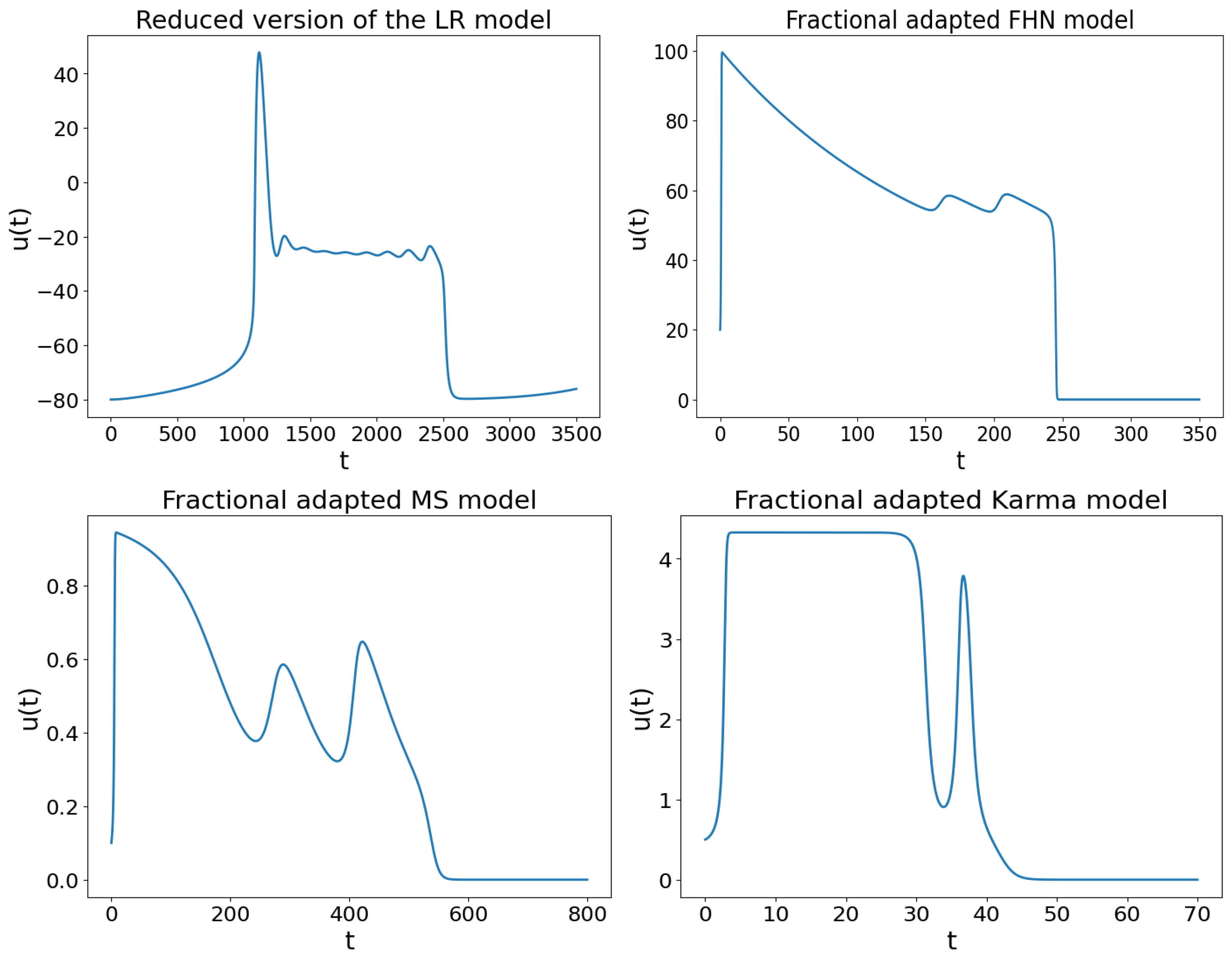
Figure 1 illustrates examples of APs with EADs in the 3D reduced version of the Luo-Rudy model [7] and in the three 2D fractional models presented in this paper.
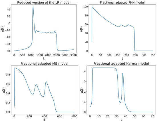
Figure 1.
EADs’ emergence were observed in a simplified 3D version of the Luo-Rudy model [7] and in the 2D fractional models based on the adapted FitzHugh-Nagumo, Mitchell-Schaeffer, and Karma cardiac models.
3.1. Fractional FitzHugh-Nagumo Model
We utilize the FHN equations [35] to model the ionic current. The solution waveform of the FHN system exhibits a hyperpolarization of the potential in the refractory period. However, this feature is not characteristic of the myocite cardiac AP and may negatively impact the model’s recovery properties, particularly in reentrant activation patterns. Therefore, to adapt the model to the problem of cardiac AP, the hyperpolarization is suppressed using an adaptation first presented by Rogers and McCulloch in 1994 [21], leading to the following equations:
where G, , and are positive coefficients, I is the input current, is the threshold and is the peak potential. We have and .
Consider . The function w implicitly incorporate past values of the voltage with an exponential weighting. In fact, the system of ODEs Equations (29) and (30) is equivalent to the following:
We write the model with a general delay kernel :
Using the gamma Mittag-Leffler PDF (6) as , Equations (26) and (27) allow to obtain the generalized fractional FHN model
If and , we recover the classic case. We consider the initial conditions and to account for the initial input current.
When we use the gamma Mittag-Leffler probability density function to generalize the memory kernel, it allows for the formation of EADs. The following simulations are conducted with a set of parameters largely derived from [20]:
Looking for minimal models in which EADs emerge, we obtain the possibility of this phenomenon with simple Mittag-Leffler distributed delays. This occurs when , and in Equation (34):
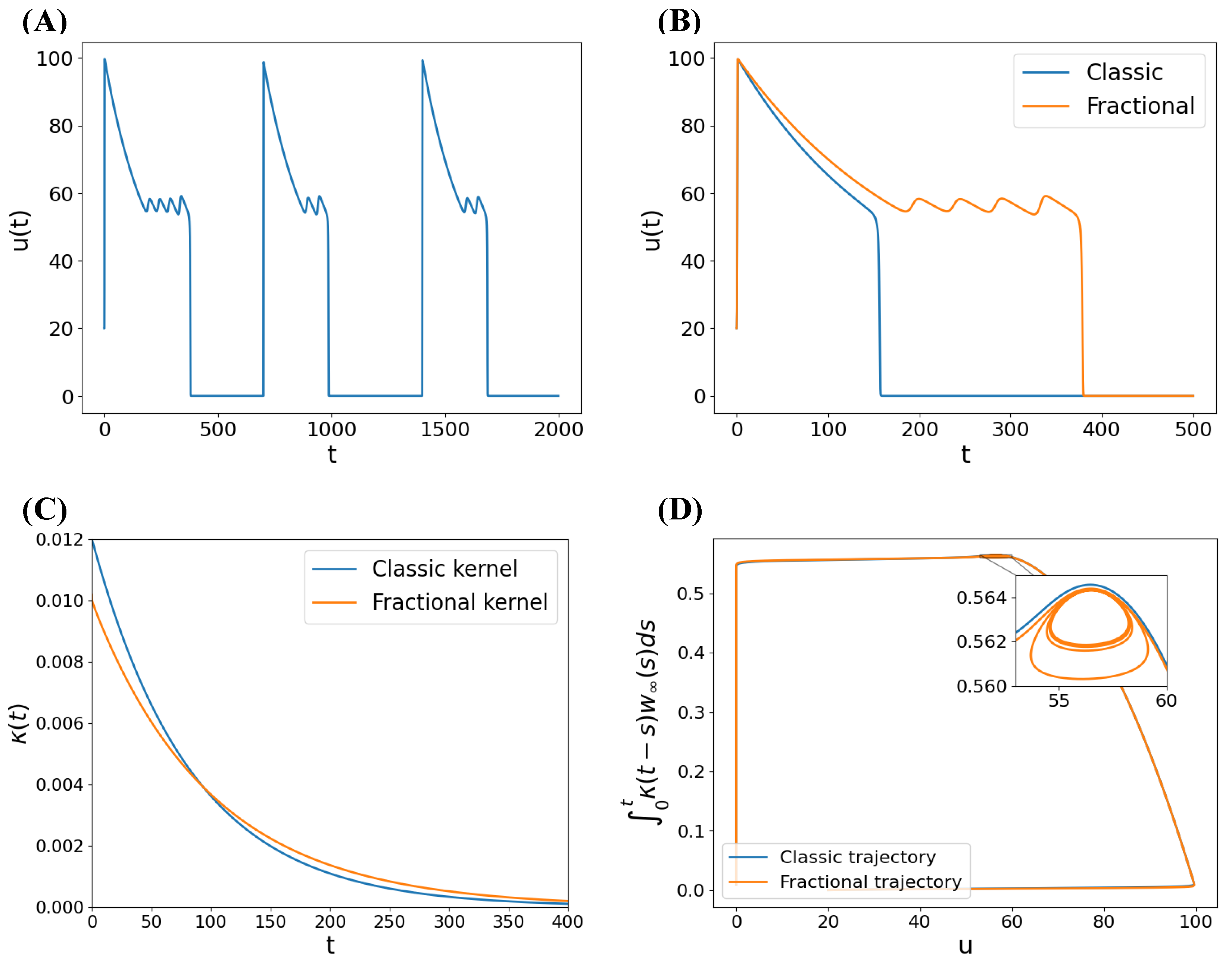
In this case, there are no finite mean and variance [18], although the memory kernel can be close to exponential during the AP interval. Figure 2A shows the emergence of EADs when , with a pace of . Note that the number of spikes of the first AP is different, but the next APs also present EAD. The comparison of the classic and the new AP is illustrated in Figure 2B,C compares the memory kernels. The fractional AP has a slower initial repolarization than the classic AP, which relates to a smaller numerical mean in the first moments. In fact, for a shorter delay, the gating variable w relates to an recent smaller voltage and can be relatively weaker than the expected. Once , the memory kernel is singular. The singularity is not evident because the kernel decreases really fast at first moments. The fractional and classic trajectories are compared in Figure 2D. The autointersections of the fractional trajectory is clear. It is important to highlight that the second coordinate when we plot the trajectories is the convolution of Equation (24). We cannot compare the w variable directly, because w was redefined between Equations (25) and (27).
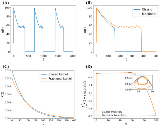
Figure 2.
Solution of the model (36) with Mittag-Leffler memory kernel, for parameters , , and . (A) AP with EADs emergence for three stimuli at a pace of 700 ms. (B) Comparison of memoryless AP and AP with EADs emergence, showing slower initial repolarization in the latter. (C) Comparison of exponential and Mittag-Leffler distributed memory kernels given by . The fractional memory kernel is singular once , but decreases rapidly initially. However, they intersect, and the fractional kernel surpasses the exponential kernel. (D) Comparison of classic and fractional trajectories, showing autointersections in the latter.
Another possibility is when and , which corresponds to a simple gamma memory kernel. In this case, the fractional Riemann- Liouville derivative only appears in the differential equation of the voltage:
We can also obtain EADs when . In this case, the fractional Riemann-Liouville derivative only appears in the differential equation of the slow variable:
Examples of the emergence of EADs for these specific simplifications and other combinations are shown in the Appendix B. In the following subsections, we propose to adjust two other two-variable cardiac models, namely the MS and Karma models, to have a phase portrait similar to the FHN cardiac model discussed earlier, thus exhibiting similar properties. This adaptation, along with the incorporation of the gamma Mittag-Leffler PDF delay kernel, enables these models to also exhibit the emergence of EADs.
3.2. Fractional Adapted Mitchell-Schaeffer Model
In [22], Mitchell and Schaeffer introduced and studied a model for electrical activity of the cardiac membrane with an inward and an outward current. The model contains two functions of time, the transmembrane potential or voltage and a gating variable , and they satisfy the following ordinary differential equations:
We propose a model which we call an adapted version of the MS model, described by
We should consider the initial conditions and to account the initial input current. However, the initial condition is not consistent with the convolution described in Equation (19). To address this, we suggest a variable transformation to ensure that . The model is reformulated as
The following simulations are conducted with a set of parameters largely derived from [22]:
The described method of generalization via gamma Mittag-Leffler PDF kernel (see Equations (26) and (27)) leads to the fractional model
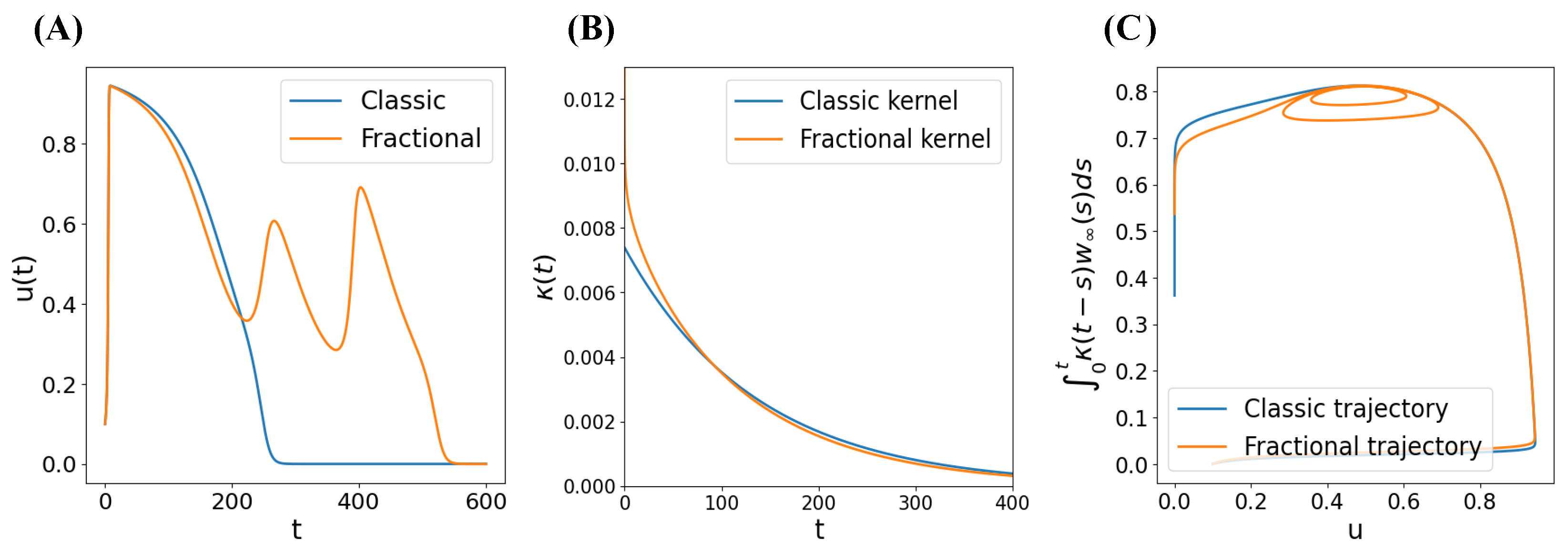
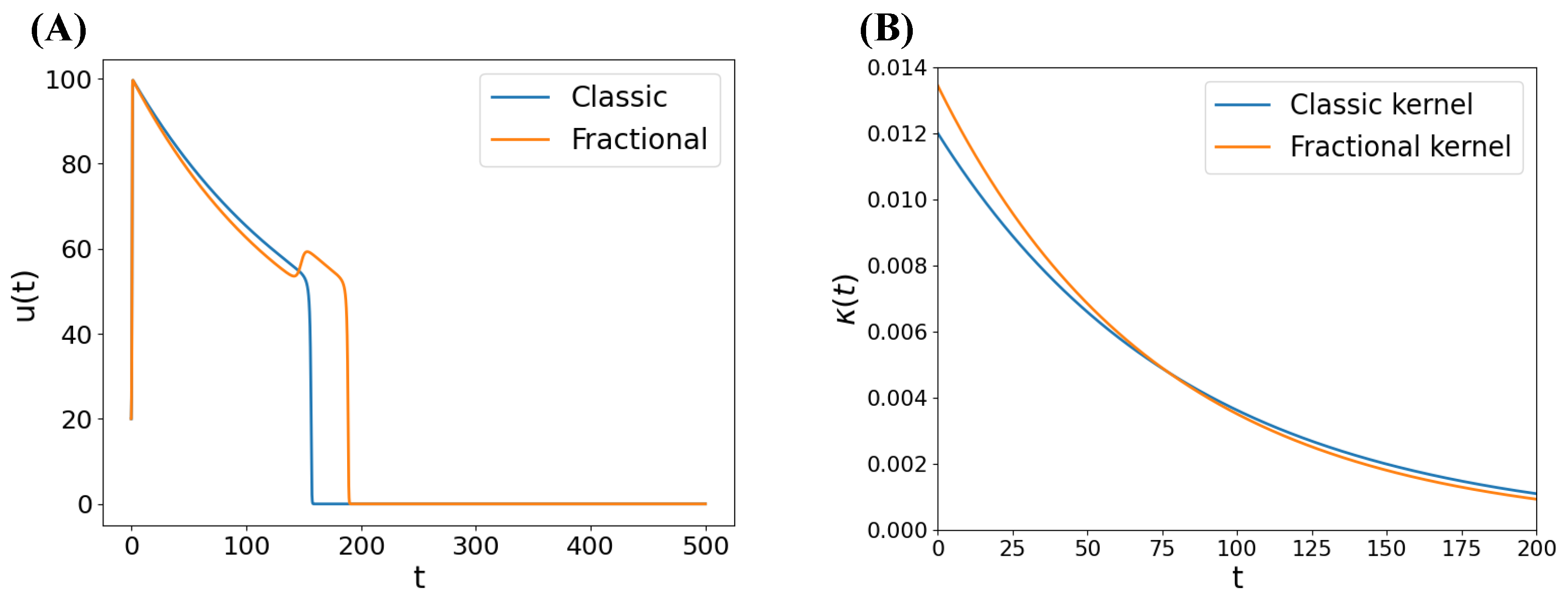
When we generalize the memory kernel with the gamma Mittag-Leffler probability density function, EADs formation is enabled. An example is illustrated in Figure 3A. Figure 3B compares the kernels. Once , the gamma Mittag-Leffler kernel is singular, and is above the classic memory kernel in the beginning. It crosses the classic kernel near to 100 ms. Finally, the comparison between the fractional and the classic trajectory is depicted in Figure 3C. Note that the fractional AP is faster in the initial repolarization. This is related to a greater numerical mean in the first moments, as cited above.
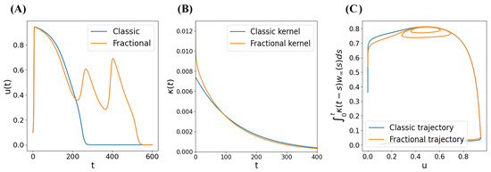
Figure 3.
Solution of the model Equation (47) with gamma Mittag-Leffler distributed memory kernel, for parameters , , , . (A) Comparison of memoryless AP and AP with EADs emergence. (B) Comparison of exponential and gamma Mittag-Leffler distributed memory kernels. The fractional memory kernel is singular once , but decreases rapidly in the time interval of interest and they intersect. (C) Comparison of classic and fractional trajectories, showing autointersections in the latter.
3.3. Fractional Adapted Karma Model
The Karma model is based on an analysis of the Noble model where the fast gate variables have been eliminated adiabatically. The model consists of two variables, a fast variable related to the membrane voltage and a slow gate variable. This model was first developed in [23] by Alain Karma (1993), to show spiral wave breakup due to alternans. The fast variable u represents the voltage, and w represents the sodium slow inactivation and potassium slow activation which are combined by the Heaviside step function:
where . The wave-front insensitivity is controlled by the parameter , i.e., the extremely weak dependence of the wave-front velocity on the slow variable, which controls the action potential duration.
We propose a model which we call an adapted version of the Karma model, described by
We consider the initial conditions and to account the initial input current. Most parameters of the following simulations are based in [23,24,25,26,27,28,29,30,31,32,33,34,35,36]:
The described method of generalization via gamma Mittag-Leffler PDF kernel (see Equations (26) and (27)) leads to the fractional model
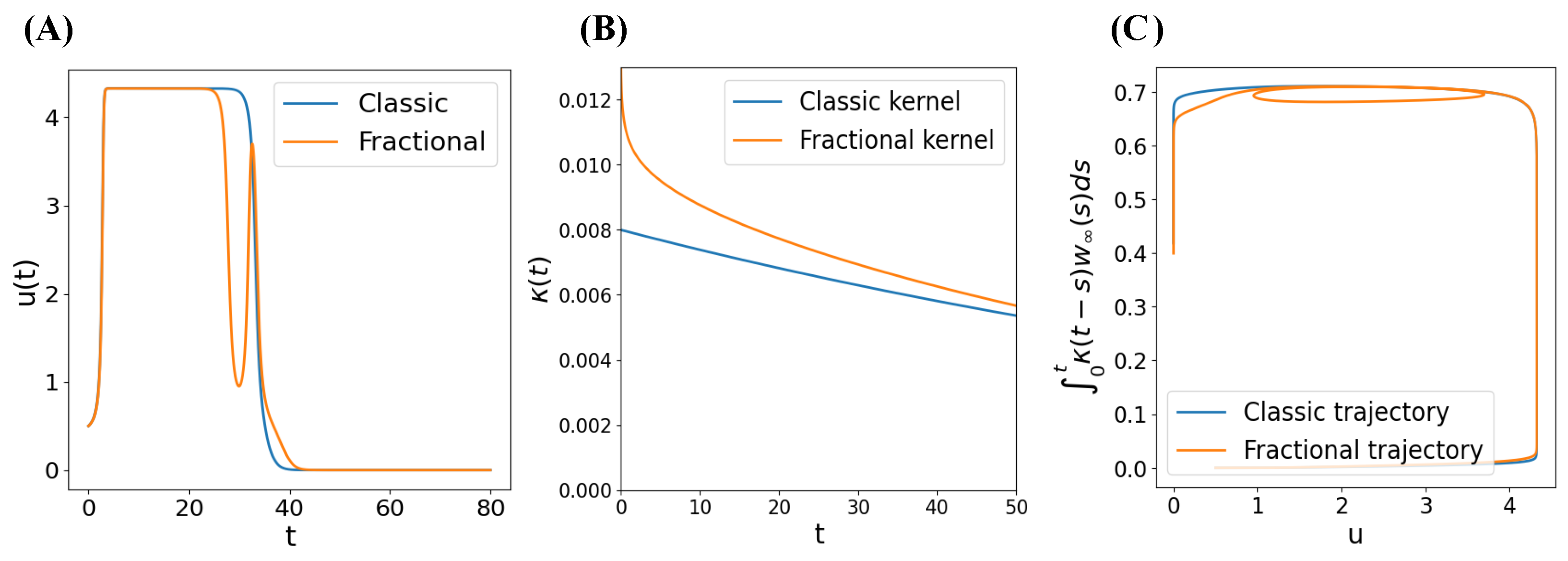
When we use the gamma Mittag-Leffler probability density function to generalize the memory kernel, it enables the formation of EADs. An example is shown in Figure 4A. Figure 4B compares the different kernels. Once , the fractional kernel is singular, but it decreases rapidly and remains smaller than the exponential kernel within the interval of interest. The comparison between the fractional and the classic trajectory is presented in Figure 4C. It is also possible to note that the fractional AP is faster in the initial repolarization. This is related to a greater numerical mean in the first moments, as cited above.

Figure 4.
Solution of the model Equation (53) with gamma Mittag-Leffler distributed memory kernel, for parameters , , . (A) Comparison of memoryless AP and AP with EADs emergence. (B) Comparison of exponential and gamma Mittag-Leffler distributed memory kernels. The fractional memory kernel is singular once and it stays above the exponential kernel in the time interval of interest. (C) Comparison of classic and fractional trajectories, showing autointersections in the latter.
4. Discussion of Earlyafterdepolarizations’ Emergence
4.1. Sensitivity Analysis
It is challenging to comprehensively explain the roles of the four parameters and as they are interrelated in a complex way. We choose the generalized fractional FHN model Equation (34) to study EADs’ emergence. For a first analysis, we consider and , the Mittag-Leffler simple case described in Equation (36) and in Figure 2. The corresponding memory kernel is given by
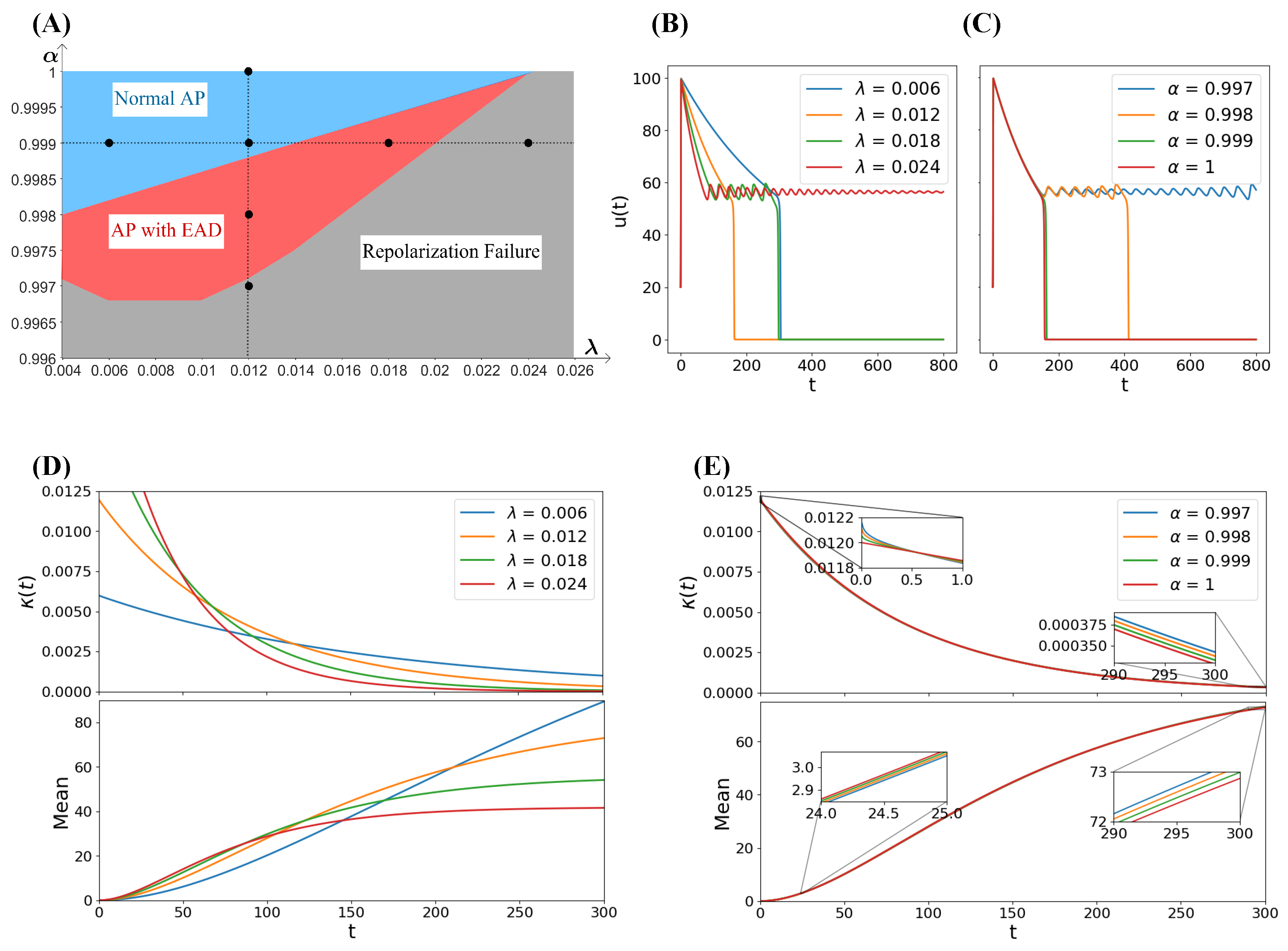
Figure 5A shows a sensitivity analysis and the region of EADs’ emergence. We analyzed simulations with and values of 0.006, 0.012, 0.018, and 0.024, represented by the large black dots on the horizontal dotted line in Figure 5A. From a typical AP for with Mittag-Leffler memory kernel, EADs can emerge if we decrease or increase . In Figure 5B, it is evident that as increases, the likelihood of EADs or repolarization failures increases, while the initial repolarization phase becomes faster. This particular type of kernel cannot be studied in terms of mean and variance, once they are infinite when , but some useful insights arise from the numerical mean. Figure 5D illustrates the relationship between and the numerical mean of the kernel: , over time. This correlation is expected since represents the time constant of the Mittag-Leffler part of the kernel, which extends the exponential function and is completely monotonic with parameters and . Furthermore, the kernels exhibit higher values at initial times when is greater. As , all the kernels are singular at zero. We observe that a higher mean in the first moments corresponds to a faster initial repolarization as increases.

Figure 5.
Simulations for the Mittag-Leffler simple case described in Equation (36) and in Figure 2. The standard case is obtained if and . (A) Regions of normal AP, AP with EAD and repolarization failure in the plane . (B) Effect of in AP behavior with memory kernel Equation (54). (C) Effect of in AP behavior with memory kernel Equation (54). (D) Effect of in the memory kernel Equation (54). Once , the kernels are singular. (E) The slight effect of in the memory kernel Equation (54).
Subsequently, we investigated simulations with and values of 0.997, 0.998, 0.999, and 1, denoted by the large black dots on the vertical dotted line in Figure 5A. Figure 5C indicates that the initial repolarization phase remains consistent across these parameter values. This similarity is supported by Figure 5E, where the kernels and their means show minimal variation during the initial repolarization.
We consider now and , the gamma simple case described in Equation (37) and in Figure A2. The memory kernel is given by
This type of kernel is extensively discussed in terms of mean and variance in the next section. Figure 6A shows the sensitivity analysis and the region of EADs’ emergence. The standard case is obtained if and . We analyze the simulations generated with and a values of 0.002, 0.01, 0.018, and 0.024, represented by the large black dots on the horizontal dotted line in Figure 6A. In general, for a typical AP with and gamma memory kernel, EADs can emerge when we decrease or increase a. In Figure 6B, it is evident that as a increases, the likelihood of EADs or repolarization failures increases, while the initial repolarization phase becomes faster. This relationship between a and the mean of the kernel is further illustrated in Figure 6D, where the time constant a influences the kernel’s behavior. The kernels exhibit higher values at initial times when a is larger, as expected due to a being the time constant of the exponential part of the kernel. Additionally, when , all the kernels become singular. Also, an increase in a results in a higher numerical mean at early times, indicating a faster initial repolarization phase. Note that the exact mean of the kernel decreases when a increases.
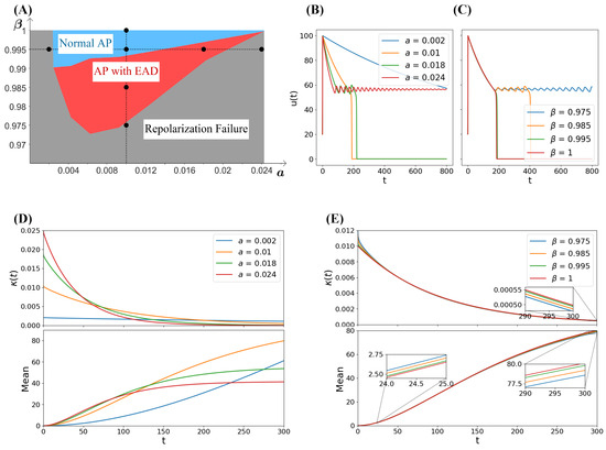
Figure 6.
Simulations for and , the gamma simple case described in Equation (37) and in Figure A2. (A) Regions of normal AP, AP with EAD and repolarization failure in the plane . (B) Effect of a in AP behavior with memory kernel Equation (54). If a is so small, there is no final repolarization until 800 ms. (C) Effect of in AP behavior with memory kernel Equation (54). The initial repolarization remains similar. (D) Effect of a in the memory kernel Equation (55). (E) Effect of in the memory kernel Equation (54). The means are very close at the beginning, but over time, it becomes apparent that the smaller the , the lower the average.
Subsequently, we investigate the simulations generated with and values of 0.975, 0.985, 0.995, and 1, denoted by the large black dots on the vertical dotted line. Figure 6C reveals that the initial repolarization phase remains consistent across these parameter values. Note from Figure 6E the similarity between the kernels and the means. The exact mean decreases when decreases.
These two simple cases illustrate the richness of the generalized fractional FHN model with respect to the shape of the memory kernel and the behavior of the AP.
4.2. The Emergence of EADs in Terms of Mean and Variance
The aim of this section is to describe the emergence of EADs in terms of the mean and the variance of the memory kernel. For this, we consider and , the gamma simple case described in Equation (37) and in Figure A2. Its memory kernel is given by Equation (55).
This choice is interesting because, while it simplifies the study of the kernel, it retains important aspects of its generality. In fact, given any positive real values and , there exist parameters a and such that the mean and variance of the gamma memory kernel are, respectively, and . For this, given and , we should consider
Note that the classic exponential memory kernel is obtained when . In the plane mean × variance, this corresponds to the parabola . Above this parabola, and the memory kernels are weak, singular at the origin. Conversely, below this parabola, and the memory kernels are strong and non-singular. For a fixed , when the memory kernel converges to the Dirac delta centered in . In this case, the model Equation (37) turns into the DDE
When and , the memory kernel converges to the Dirac delta centered in 0, and the model Equation (37) turns into the ODE
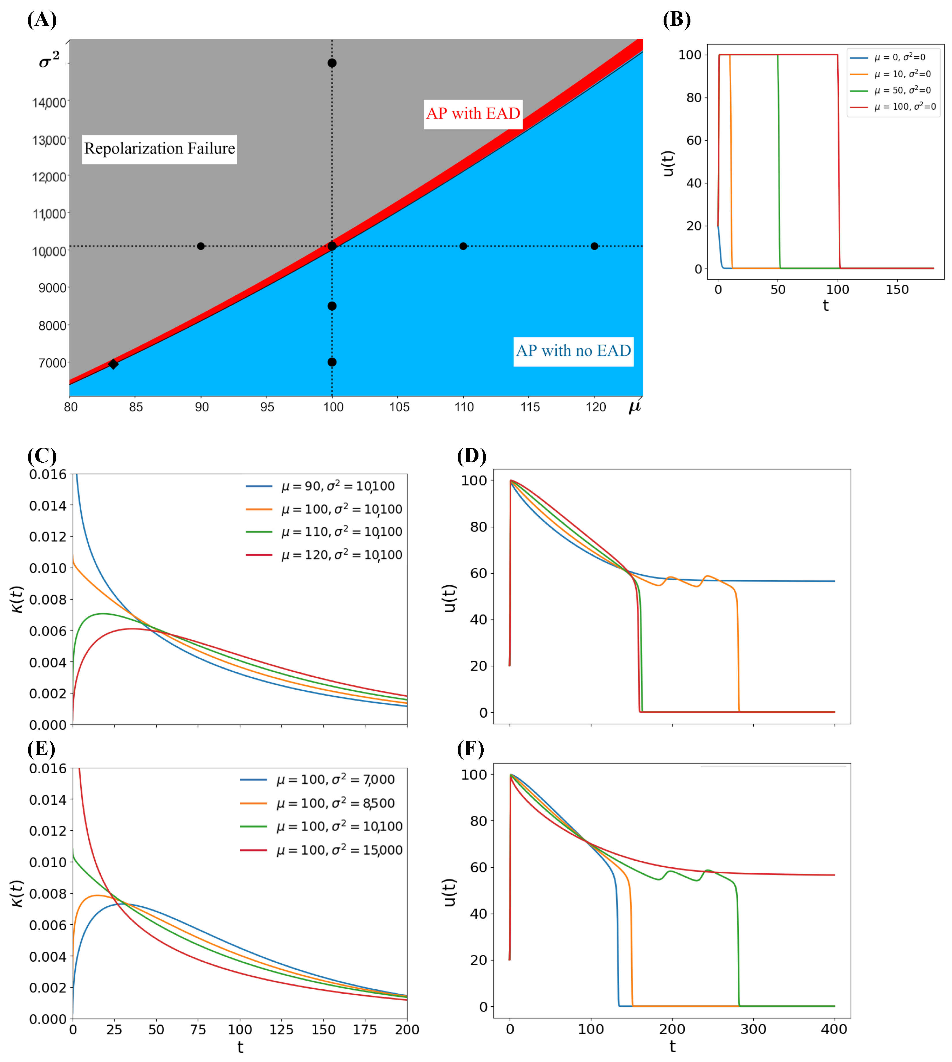
Figure 7A shows three regions of the mean × variance plane. First, we have a region where there are complete APs. At its lower limit are the Dirac delta memory kernels. Then, there is a region in which the APs present EADs, culminating in a region of repolarization failure. The region with EADs’ emergence (red region) is practically non-existent for small means. Figure 7B illustrates the limit case with Dirac delta kernels, described in Equation (57). When , the model comes down to the ODE (58) and there is no depolarization. Figure 7C illustrates APs generated by the kernels corresponding to the black points in Figure 7A, going through the regions in a vertical slice. Note that the mean is the same, and as the variance increases, the AP duration increases and the final repolarization becomes more difficult.
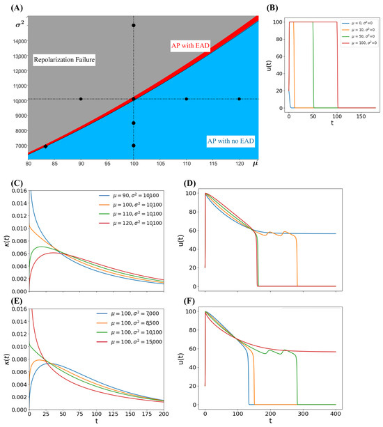
Figure 7.
Simulations for the gamma simple case described in Equation (37) and in Figure A2, respecting the relation Equation (56). The standard case is obtained in the black diamond, in which and . (A) Regions of normal AP, AP with EADs and repolarization failure in the plane . For each , if increases, there is a small interval where EADs occur. Then, if increases more, there is a repolarization failure. The black parabola corresponds to the integer cases in which . (B) Special case in which the model is described by the DDE (57). When , the model comes down to the ODE (58). When , the behavior of the model is like a square wave with length . (C) Gamma kernels generated by the black points in (A) , going through the regions in an horizontal slice. For a fixed , as decreases, the more recent past has more weight in the memory kernel. (D) APs generated by the gamma memory kernels in (C). (E) Gamma kernels generated by the black points in (A), going through the regions in an vertical slice. For a fixed , as increases, the more recent past has more weight in the memory kernel. (F) APs generated by the gamma memory kernels in (E).
The key finding of this analysis is that transitioning from the blue region without EADs to the red region with EADs can be achieved by making slight adjustments either to the left (lower mean) or upwards (higher variance). A leftward shift indicates a smaller mean in the kernel, suggesting a shorter memory, while moving upwards maintains the mean but increases the variance, causing the kernel to shift towards the origin (see Figure 7).
Biologically, EADs can occur when repolarization reserve is reduced due to a decrease in outward current, an increase in inward current, or both, compromising the net outward current needed for myocyte repolarization [37]. In the modified FHN models, the fast variable represents the transmembrane voltage, while the slow variable is associated with potassium channel activation. During repolarization, the membrane voltage decreases, and the slow variable follows this change with a delay. If this delay is shortened, the slow variable tracks the decreasing voltage more rapidly, resulting in a lower potassium current because the earlier voltage is smaller. This premature decline in the potassium current can make the membrane more susceptible to reactivation by inward currents, increasing the likelihood of early afterdepolarizations.
Shifting to the left or upwards in the mean × variance plane makes the potassium current more dependent on recent voltage values, as the mode of the memory kernel’s PDF moves closer to the present. These adjustments accelerate the potassium current response during repolarization, increasing the likelihood of EADs and potentially causing repolarization failure. There is a narrow parameter range where EADs can emerge between normal action potentials and complete repolarization failure, enabled by the fractional-order formulation allowing trajectories of the system to intersect.
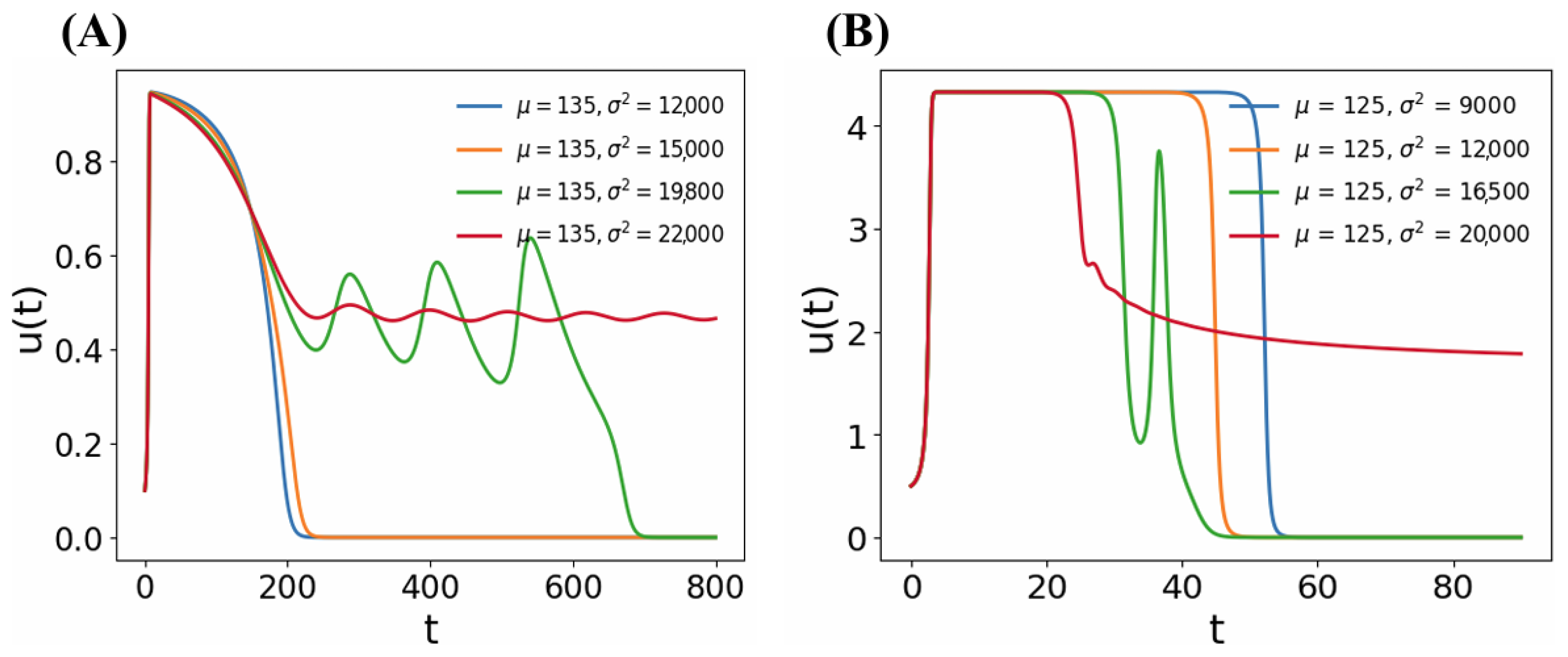
Figure 8 shows similar results for the MS and Karma fractional models with gamma memory kernel. However, in these models, the biological interpretation differs from the above. In the fractional MS model (Equation (47)), the convolution is associated with the inactivation of inward current (whether sodium or calcium). When the memory distribution considers a more recent past, the inward current increases temporarily due to lower recent voltage values compared to distant ones during initial repolarization. This shifts the action potential and leads to the emergence of EADs. A similar behavior is observed in the fractional Karma model (Equation (53)).
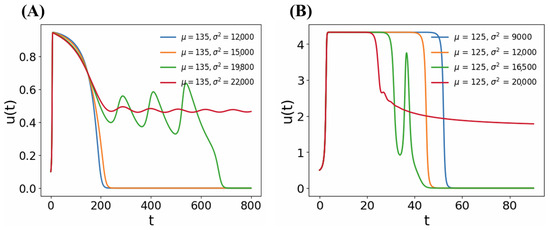
Figure 8.
(A) APs generated by MS fractional model Equation (47) with gamma kernel described by Equation (56). (B) APs generated by Karma fractional model Equation (53) with gamma kernel described by Equation (56). Maintaining the mean while the variance increases, the final repolarization becomes more difficult in both cases.
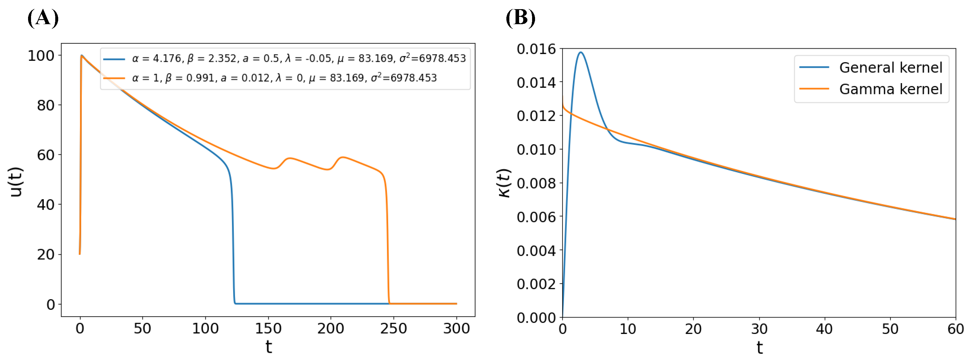
We hypothesize that similar insights can be applied to the general gamma Mittag-Leffler PDF memory kernel, where the parameters and are not constrained, except for the requirement of the PDF’s existence. However, a general approach is not easy to establish. Some kernels can be effectively described using a gamma kernel, but not all. Figure 9 illustrates two different APs generated for Equation (34) with kernels of same mean and variance, the first with four free parameters related to the fractionalization, and the second a gamma kernel. Note that the general kernel exhibits a behavior that cannot be captured with a gamma kernel. More discussion about the richness of the general kernels can be found in [18].
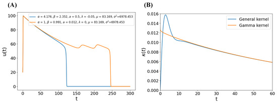
Figure 9.
(A) APs generated by FHN fractional model Equation (34). (B) Respective memory kernels, with the same mean and variance.
4.3. Stability Analysis
From a stability analysis perspective, the transition from repolarization failure to complete action potential is attributed to a change in stability. Our simulations indicate that EADs in the fractional generalized model result from unstable focus or unstable limit cycles observed in the corresponding integer model. In this context, we consider the time scale as the bifurcation parameter in the integer order model Equation (34), and fix in their corresponding fractional model Equations (29) and (30).
First, we prove that the fractional system Equation (34) has the same equilibrium point as its equivalent integer system (29) and (30). Although this is trivial when the integer order derivative is replaced with the Caputo fractional derivative, the equilibrium computation when the fractional Riemann-Liouville derivative arises from an integrodifferential perspective is not immediate. In [38], we see an example in which the equilibrium of the fractional equation are not the same of its integer counterpart.
4.3.1. Equilibrium Points
The system (29) and (30) has a trivial equilibrium given by . We discuss non-trivial equilibria. Note that in equilibrium, we must have . Then, if , the equilibrium must satisfy
This is a quadratic equation in u, and can be written as
Thus, the system can present at most two non-trivial equilibria given by
where
Now, we aim to calculate the equilibrium points of the fractional system (34). From a known result under some assumptions (see, e.g., [38]), the following asymptotic behavior is derived:
Beyond the null equilibrium , we must have
By definition, we obtain
4.3.2. Stability
We study the stability of the integer order system (29) and (30). First, we calculate the Jacobian matrix:
In a non-null equilibrium , we have
Then, the trace of the Jacobian matrix in an equilibrium is given by
In the next step, we compute the determinant of the Jacobian matrix. In an equilibrium , it is given by
Thus, in a non-null equilibrium, occurs if, and only if,
Thus, when it exists, is a saddle point. With respect to , its existence states that it is an unstable point if and only if , which means
Once the determinant signal does not depend on , there is a Hopf bifurcation with respect to when for .
The stability analysis of the equilibrium of the fractional system is not trivial, although the ad hoc replacement of the Caputo fractional derivative in an integer model can have its stability analyzed in a simpler manner [39]. Progress in stability studies can be made using integral formulations of the model [38], which is beyond our current scope.
4.3.3. Emergence of EADs
Recent results (see, for instance, [16,17]) point that oscillatory states in fractional model arise when a bifurcation parameter is taken near Hopf-like bifurcation points. The concept of Hopf-like arises due to the impossibility of a fractional model to undergo a classic Hopf bifurcation; in fact, a fractional system cannot have exact periodic solutions [40]. However, this concept is used in when the integer derivative is replaced on the left side of the ODEs with Caputo fractional derivative. This is not the present case, but we can get some insight taking in hand simulations results and the stability classification of the integer order counterpart.
Note that the expression
is positive exactly in the interval . This result, together with Equation (77), indicates that a Hopf bifurcation occurs when , i.e., when
If is slightly greater than , the equilibrium point of the integer model is an unstable spiral. A subcritical Hopf bifurcation occurs in and there is an unstable limit cycle when is slightly smaller than . It is in this neighborhood that EADs were observed in our simulations.
Particularly, with gamma memory kernels, if we fix , the mean and the variance are related in the form . EADs were observed when and . For the parameters of Equation (35), independently of value, we have .
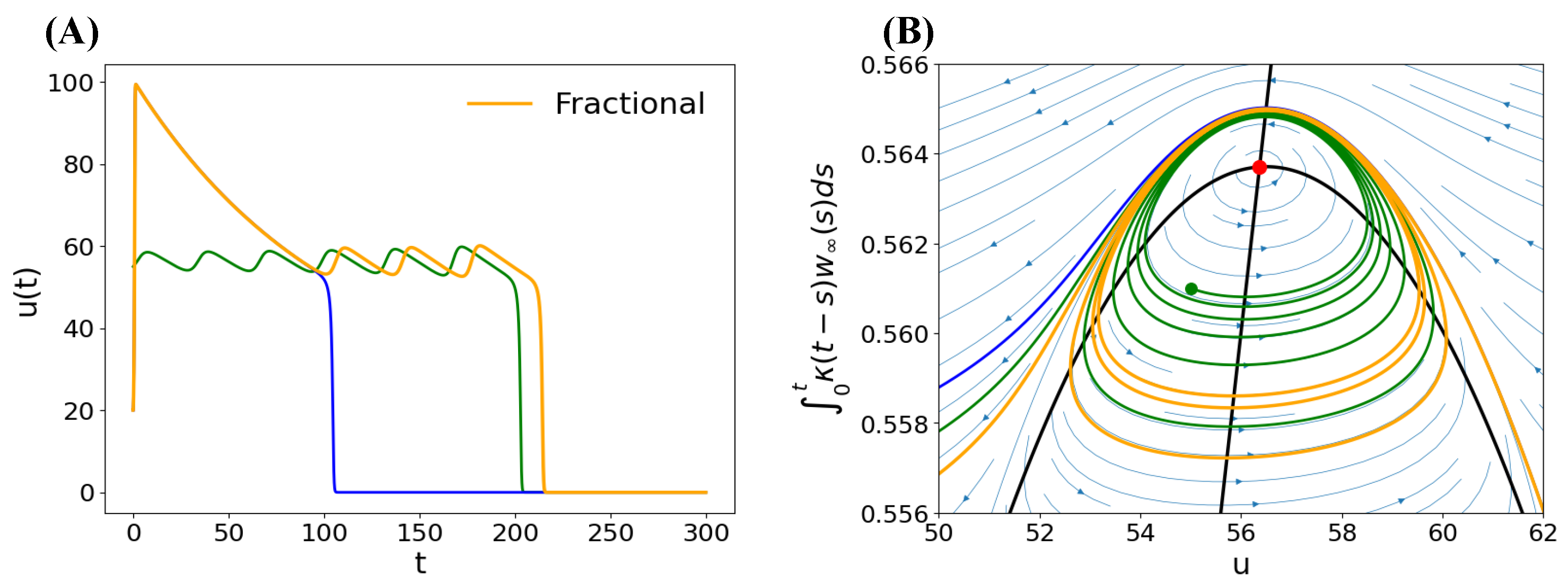
In Figure 10, we show the behavior of two integer-order solutions and a fractional one. The equilibrium point, in red, is an unstable spiral of the integer model. Although the fractional trajectory may enter the spiral region, the non-autonomous nature of the equation allows it to escape and continue evolving. In this example, the yellow fractional and blue classic trajectories have the same initial point and coincide until the neighbor of the equilibrium point.
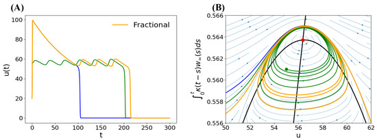
Figure 10.
The phase portrait of the solutions in (A) is plotted in (B) with the parameters of Equation (35), but , so . For the simulation of the fractional model, we consider . The nullclines of the integer-order model are depicted in black, and the red dot is the equilibrium . The green small dot indicates the initial point of the green trajectory, that spirals outwards. The initial condition for the fractional yellow and the blue trajectories is .
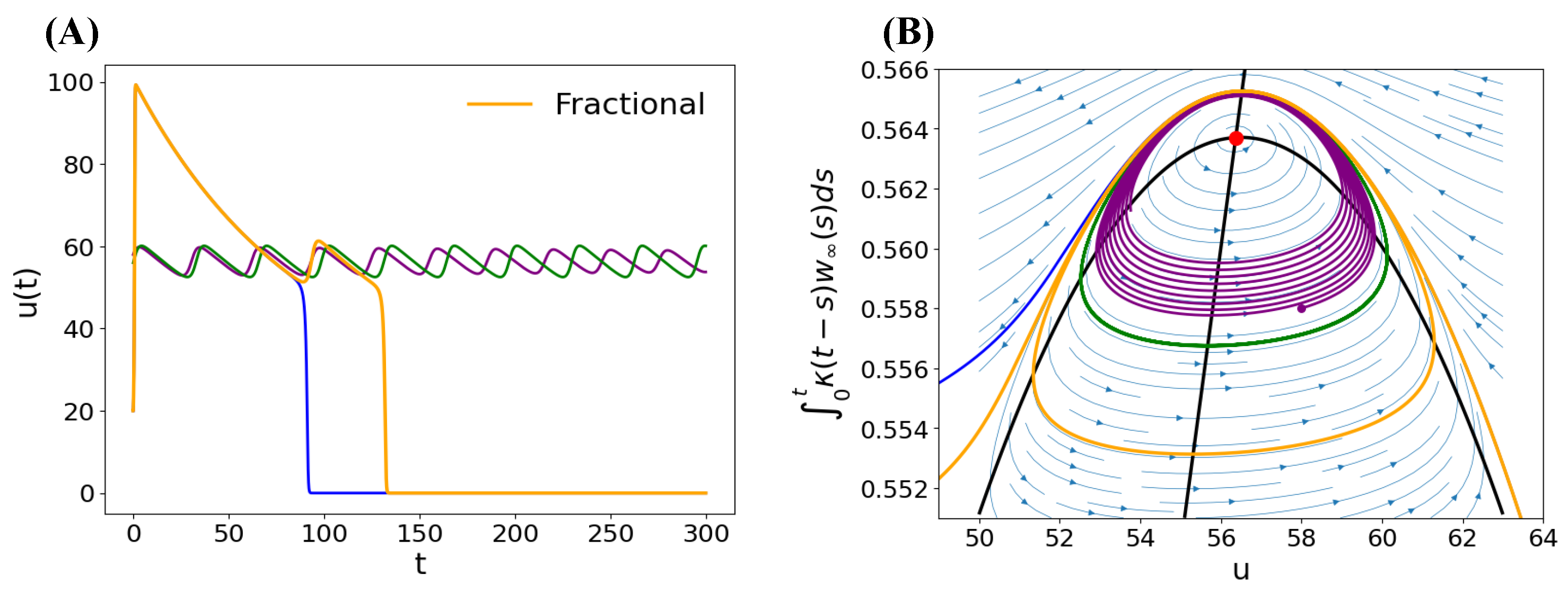
In Figure 11, we show the case in which there is an unstable limit cycle. The equilibrium point, in red, is a stable spiral of the integer model. The purple solution moves away from the green one, the limit cycle, showing this is unstable. Note that the fractional solution enters the spiral due to the unstable limit cycle and is free of it due to the possibility of autointersection of the trajectory. Also in this example, the yellow fractional and blue classic trajectories coincide until the neighbor of the equilibrium point.
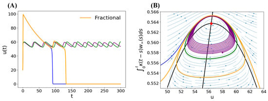
Figure 11.
The phase portrait of the solutions in (A) is plotted in (B) with the parameters of Equation (35), but , so . For the simulation of the fractional model, we consider . The nullclines of the integer-order model are depicted in black, and the red dot is the equilibrium . The purple small dot indicates the initial point of the purple trajectory, that spirals inwards. The initial condition for the fractional yellow and the blue trajectories is .
These stability observations support the modifications made to the MS and Karma models, as detailed in Appendix C.
5. Discussions and Conclusions
This study exhibits and discusses the emergence of EADs by altering the memory kernel of the slow variable in simple two-variable models using tools from Fractional Calculus. To this aim, we developed a mathematical protocol with which Hodgkin-Huxley type equations can be extended with gamma Mittag- Leffler distributed delays, resulting in fractional models. With this construction, two-variable adapted FitzHugh-Nagumo, Mitchell-Schaeffer and Karma cardiac models generate mixed-mode oscillations that can be named as EADs. This phenomenon can only be described by autonomous systems of ODEs with at least three variables.
One of the major challenges recent discussed Fractional Calculus is to determine how, where and why fractional derivatives interfere in the models [41,42]. Recent studies as [18,19,43] advanced towards presenting constructive methods for fractional modeling, establishing where the fractional functions are acting in the model (waiting times, delay kernels, etc.). We followed this type of construction in the current work.
There are four parameters that raise in the fractional extension of the models: and . The time constant is not present in the generalized model, but then a and are generally related to it. To achieve the aim of discuss the intrinsic relation of the memory kernel and the generated AP, we conducted a thorough analysis of the sensitivity of parameters for two specific instances of memory kernels: namely, Mittag-Leffler and gamma memory kernels. Then, the emergence of EADs is characterized by changes in the mean and variance of gamma memory kernels. The analysis reveals that transitioning from a state without EADs to one with EADs can be achieved by a slight decrease of the mean or a slight increase of the variance. Any of these two discreet shifts implies that recent voltage values have more influence on the potassium current during repolarization, leading to a temporary increase in the action potential and triggering EADs. This adjustment in the kernel’s characteristics explains the emergence of EADs during repolarization.
Furthermore, we notice that EADs occur when the fractional trajectory passes close to an unstable spiral equilibrium or limit cycle of the integer-order system. The fractional trajectory can enter the spiral but has the ability to escape due to the non-autonomous nature of fractional generalizations, allowing trajectories to intersect themselves. The significance of spiral points in the formation of EADs is consistent with previous findings, such as [44], who showed in a Luo-Rudy cardiac model that EADs arise when the nonresting steady state of the voltage/Ca current subsystem loses stability through a Hopf bifurcation, leading to oscillations terminated by a homoclinic bifurcation. The relationship between oscillations and Hopf-like bifurcations in fractional models has been explored in recent studies (e.g., [11,12,13,14,15,16,17]). It is important to note that these models differ from the presented model as they use Caputo fractional derivatives on the left side, which may lead to issues with physical interpretation, mass balance, units, positivity, and monotonicity. These concerns have been discussed in [45,46,47], and other related literature. The approach presented here addresses these issues effectively, as outlined in [18].
Future studies should investigate from a biological and measurable viewpoint the relationship between mixed-mode oscillations and the parameters and , delving into the richness of the gamma Mittag-Leffler PDF kernels. We also suggest that by utilizing integral formulations of the model, the stability studies can potentially be formalized.
Author Contributions
Conceptualization, N.Z.M., R.W.d.S. and S.R.M.; methodology, N.Z.M., R.W.d.S. and S.R.M.; software, N.Z.M.; validation, N.Z.M.; investigation, N.Z.M.; writing—original draft, N.Z.M.; writing—review & editing, N.Z.M. and R.W.d.S.; supervision, R.W.d.S. and S.R.M.; project administration, R.W.d.S.; funding acquisition, R.W.d.S. All authors have read and agreed to the published version of the manuscript.
Funding
The authors would like to express their thanks to FAPEMIG, FINEP, CAPES, CNPq and UFJF.
Data Availability Statement
Dataset (codes) available on request from the authors.
Conflicts of Interest
The authors declare no conflicts of interest. The funders had no role in the design of the study; in the collection, analyses, or interpretation of data; in the writing of the manuscript; or in the decision to publish the results.
Appendix A. Study of the Gamma Mittag-Leffler PDF Kernel
In this Appendix, we discuss how the parameters and impact the memory kernel given in Equation (6).
Figure A1A,B presents how and impact the memory kernel for and , which are chosen from simulations of the fractional FHN model (see Section 3). To analyze the effect of in Figure A1A, we keep constant at . Decreasing causes the kernel to decrease more rapidly in its initial stages, while slightly increasing the weight of the right tail. Conversely, to investigate the influence of in Figure A1B, we fix at . As increases within the specified time range, the kernel exhibits lower values at earlier times, with the right tail becoming more prominent. The kernels exhibit a singularity at time 0 when is less than 1. Note that, with the time range and the set of parameters considered, the fractional order has more impact in the memory kernel.
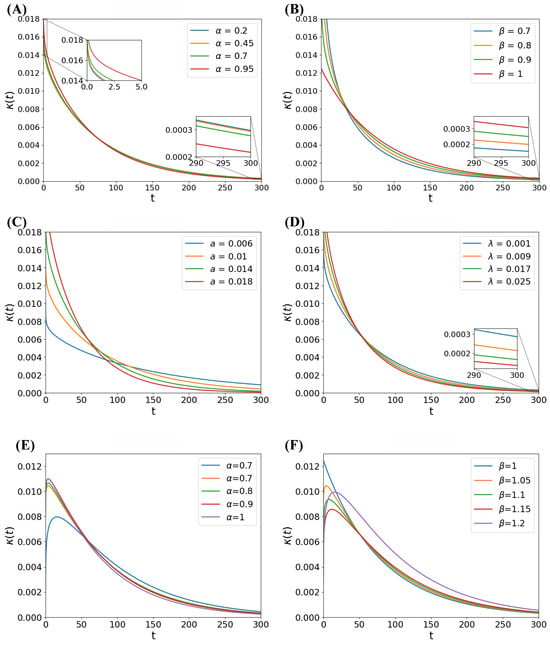
Figure A1.
For panels (A–D) we fix three of the four parameters . We consider in panel E and in panel F. In the specified time interval: (A) Effect of : Decreasing leads to a faster decrease in the kernel at the beginning, with a slightly heavier right tail. (B) Effect of : Increasing results in smaller values in the early moments of the kernel, with a heavier right tail. (C) Effect of a: Decreasing a causes smaller values in the early stages of the kernel, but a slower decay. (D) Effect of : it affects the kernel similarly to a, but with less impact. (E) Effect of —Strong kernels: Decreasing leads to a smaller peak, although most spread out with a slightly heavier right tail. (F) Effect of —Strong kernels: Decreasing causes the kernel to shift towards the origin.
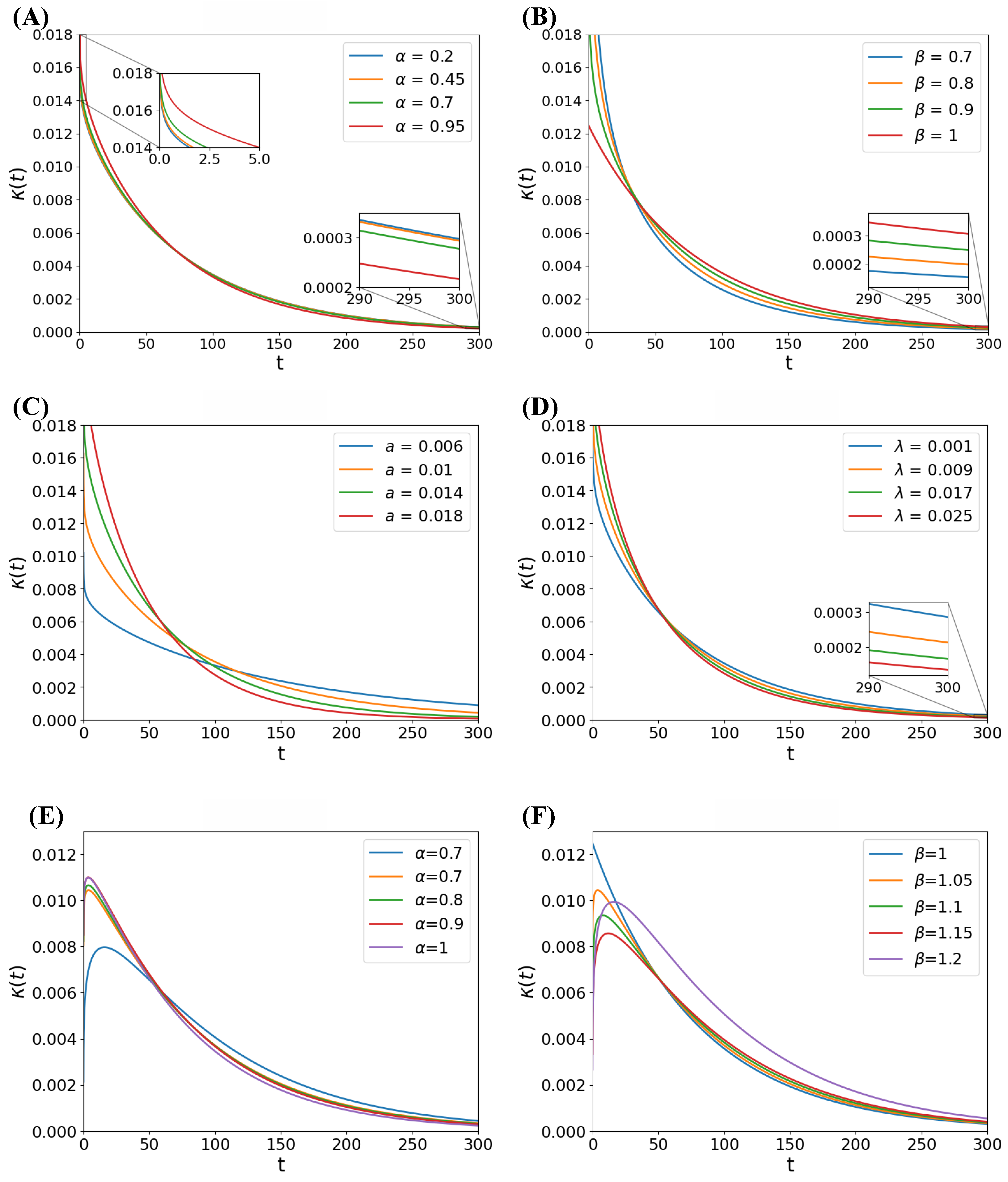
On the other hand, Figure A1C,D discusses how a and impact the memory kernel (6) for and . To analyze the effect of a in Figure A1C, we keep constant at . In the time interval of interest, as a decreases, the early stages of the kernel have smaller values, but the decay is slower. To analyze the effect of , we keep a constant at . Figure A1D shows that affects the kernel in a similar way to a, but with less intensity. The parameters a and relate to the velocity of the model and can be understood as a type of time constant.
Appendix B. EADs Examples in the Fractional FHN Model
In this Appendix, we present examples of the emergence of EADs for specific simplifications and other combinations of the fractional FHN model. Upon solving the system (37), a comparison of a classic and a modified AP is illustrated in Figure A2A, while Figure A2B compares the kernels. Once , the memory kernel is singular and, during the interest interval, the only significant difference between the kernels is in the early times. This example illustrates that EADs can occur with minimal changes of an exponential memory kernel.
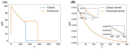
Figure A2.
Solution of the model (37) with gamma memory kernel, for parameters , , , and . (A) Comparison of memoryless AP and AP with EADs emergence, showing similar initial repolarization. (B) Comparison of exponential and gamma distributed memory kernel given by . They intersect, but are very similar. The fractional memory kernel is singular once .
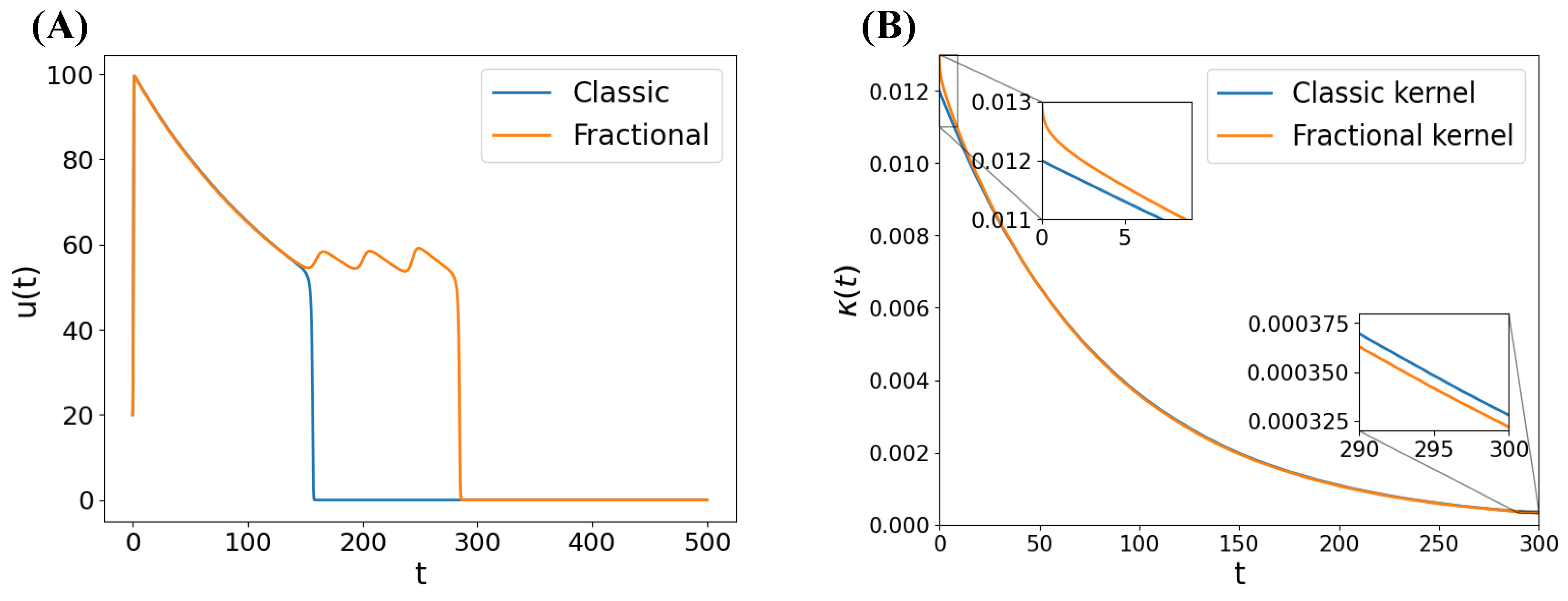
Figure A3A shows the emergence of EAD with the example in which and (system (38) and (39)). Figure A3B compares the kernels. Once , the kernel is non-singular, although it is greater than the classic kernel in the early times. Note that the fractional AP is faster in the initial repolarization. This is related to a greater numerical mean in the first moments. With a longer delay, the gating variable w corresponds to a higher voltage earlier and may be relatively greater than anticipated.
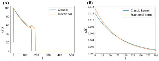
Figure A3.
Solution of the model (38) and (39), for parameters , , , . (A) Comparison of memoryless AP and AP with EADs emergence, showing faster initial repolarization in the latter. (B) Comparison of exponential and fractional memory kernel given by . The fractional memory kernel is non-singular once . In the time interval of interest, it starts above the exponential and crosses it, decaying more rapidly.
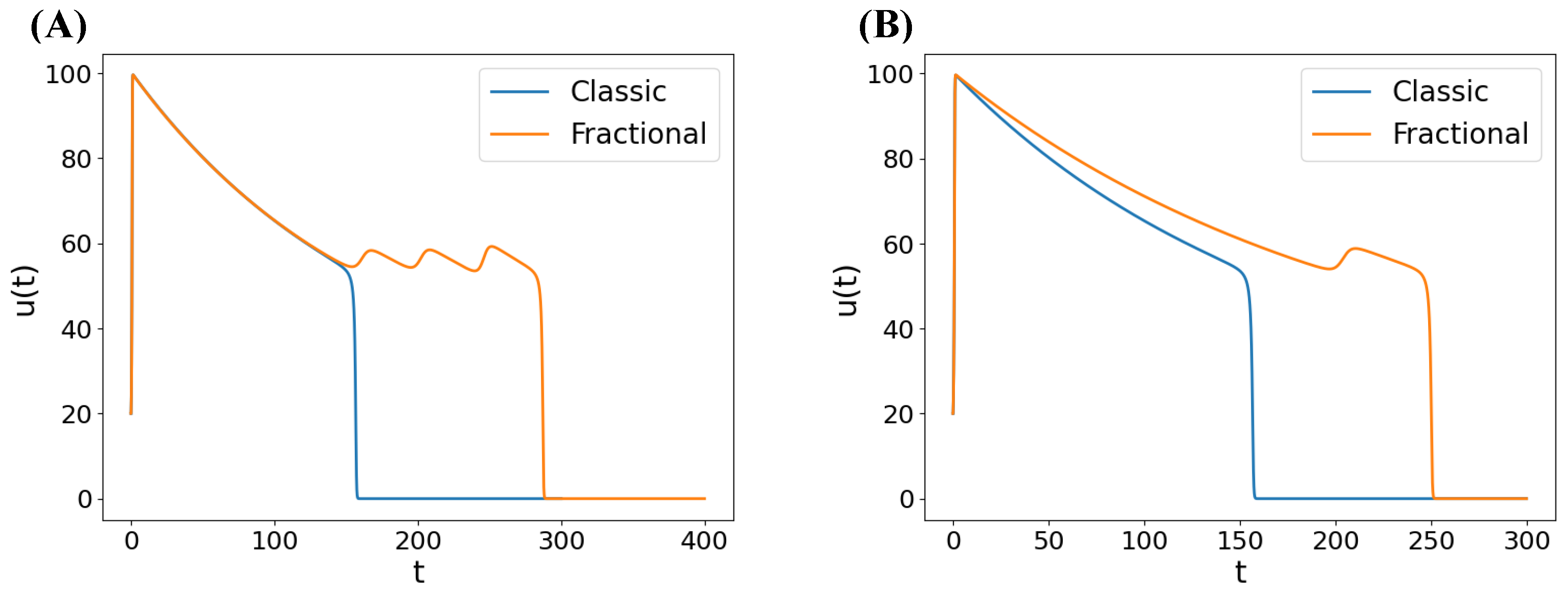
Several other combinations of parameters allow for different mixed-mode oscillations. See, for example, Figure A4.
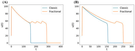
Figure A4.
(A) Comparison of memoryless AP and AP with EADs emergence, for parameters , , , . (B) Comparison of memoryless AP and AP with EADs emergence, for parameters , , , .
Figure A4.
(A) Comparison of memoryless AP and AP with EADs emergence, for parameters , , , . (B) Comparison of memoryless AP and AP with EADs emergence, for parameters , , , .
Appendix C. Justification of Our Adaptations in the MS and Karma Models
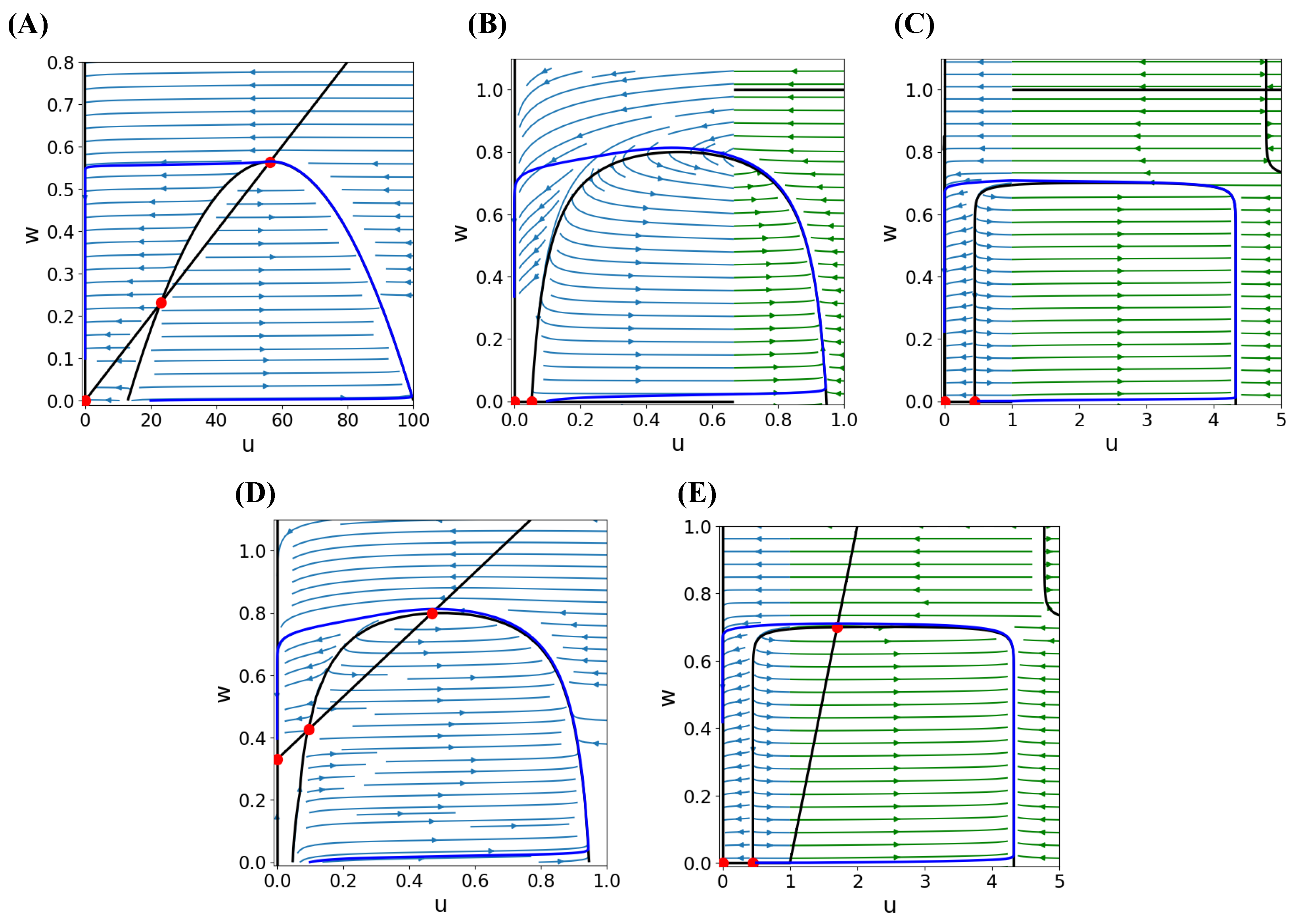
In this Appendix, we justify our adaptations in the MS and Karma models based in the stability observations discussed in the Section 4.3. Figure A5 displays the phase portraits of the integer FHN, MS, and Karma adapted models with parameter sets that induce EADs. The geometry of the phase portraits in Figure A5B,C cannot exhibit a spiral equilibrium. The adaptations of the MS and Karma models aimed to replicate the geometric characteristics of the phase portrait in Figure A5A. Numerical simulations show that the third equilibrium in Figure A5D,E are unstable spirals.
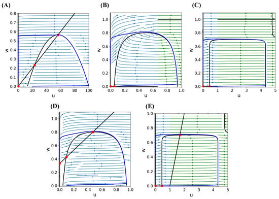
Figure A5.
Phase portraits with vector fields are shown, where nullclines are depicted in black, the model’s solution in blue, and equilibrium points as red dots. (A) Phase portrait of the integer FHN model given by Equations (29) and (30) with parameters from Equation (35). Note that are three equilibrium, with two of them arising from the intersection of a linear and a parabolic nullcline. (B) Phase portrait of the integer classical MS model with Equations (40) and (41), using the change of variable and parameters from Equation (46). There are two equilibrium in which . (C) Phase portrait of the integer classical Karma model with Equations (48) and (49), using the parameters from Equation (52). Similarly, there are two equilibrium in which . (D) Phase portrait of the integer linear MS model with Equations (42) and (43). The geometry resembles that of the FHN model, with three equilibrium, two of them on the curve nullcline (E) Phase portrait of the integer linear Karma model with Equations (50) and (51). Similar to the MS case, the geometry resembles that of the FHN model. Note that the curved nullclines are non-trivial due to the term in the first equation.
References
- Hodgkin, A.L.; Huxley, A.F. A quantitative description of membrane current and its application to conduction and excitation in nerve. J. Physiol. 1952, 117, 500. [Google Scholar] [CrossRef] [PubMed]
- Cranefield, P.F. Action potentials, afterpotentials, and arrhythmias. Circ. Res. 1977, 41, 415–423. [Google Scholar] [CrossRef]
- Charpentier, F.; Drouin, E.; Gauthier, C.; Marec, H.L. Early after/depolarizations and triggered activity: Mechanisms and autonomic regulation. Fundam. Clin. Pharmacol. 1993, 7, 39–49. [Google Scholar] [CrossRef] [PubMed]
- Huang, X.; Song, Z.; Qu, Z. Determinants of early afterdepolarization properties in ventricular myocyte models. PLoS Comput. Biol. 2018, 14, e1006382. [Google Scholar] [CrossRef]
- Stein, J.; Greene, D.; Fenton, F.; Shiferaw, Y. Mechanism of Arrhythmogenesis Driven by Early After Depolarizations in Cardiac Tissue. PLoS Comput. Biol. 2025, 21, e1012635. [Google Scholar] [CrossRef] [PubMed]
- Wang, R.; Qu, Z.; Huang, X. Dissecting the roles of calcium cycling and its coupling with voltage in the genesis of early afterdepolarizations in cardiac myocyte models. PLoS Comput. Biol. 2024, 20, e1011930. [Google Scholar] [CrossRef]
- Barrio, R.; Jover-Galtier, J.A.; Martínez, M.; Pérez, L.; Serrano, S. Mathematical birth of Early Afterdepolarizations in a cardiomyocyte model. Math. Biosci. 2023, 366, 109088. [Google Scholar] [CrossRef]
- Kügler, P.; Erhardt, A.H.; Bulelzai, M. Early afterdepolarizations in cardiac action potentials as mixed mode oscillations due to a folded node singularity. PLoS ONE 2018, 13, e0209498. [Google Scholar] [CrossRef]
- de Barros, L.C.; Lopes, M.M.; Santo Pedro, F.; Esmi, E.; dos Santos, J.P.C.; Sánchez, D.E. The memory effect on Fractional Calculus: An application in the spread of COVID-19. Comput. Appl. Math. 2021, 40, 72. [Google Scholar] [CrossRef]
- Du, M.; Wang, Z.; Hu, H. Measuring memory with the order of fractional derivative. Sci. Rep. 2013, 3, 3431. [Google Scholar] [CrossRef]
- Ngueuteu, G.; Yamapi, R.; Woafo, P. Quasi-static transient and mixed mode oscillations induced by fractional derivatives effect on the slow flow near folded singularity. Nonlinear Dyn. 2014, 78, 2717–2729. [Google Scholar] [CrossRef]
- Abdelouahab, M.S.; Lozi, R. Hopf-like bifurcation and mixed mode oscillation in a fractional-order FitzHugh-Nagumo model. In AIP Conference Proceedings; AIP Publishing: Melville, NY, USA, 2019; Volume 2183. [Google Scholar]
- Teka, W.W.; Upadhyay, R.K.; Mondal, A. Spiking and bursting patterns of fractional-order Izhikevich model. Commun. Nonlinear Sci. Numer. Simul. 2018, 56, 161–176. [Google Scholar] [CrossRef]
- Lozi, R.; Abdelouahab, M.S.; Chen, G. Mixed-Mode Oscillations Based on Complex Canard Explosion in a Fractional-Order Fitzhugh-Nagumo Model. Appl. Math. Nonlinear Sci. 2020, 5, 239–256. [Google Scholar] [CrossRef]
- Mbouna, S.G.N. Fractional Calculus-Based Generalization of the FitzHugh-Nagumo Model: Biophysical Justification, Dynamical Analysis and Neurocomputational Implications. In Nonlinear Systems-Recent Developments and Advances; IntechOpen: London, UK, 2022. [Google Scholar]
- Gao, X.L.; Zhang, H.L.; Wang, Y.L.; Li, Z.Y. Research on pattern dynamics behavior of a fractional vegetation-water model in arid flat environment. Fractal Fract. 2024, 8, 264. [Google Scholar] [CrossRef]
- He, K.; Song, J.; Zhao, N.; Liu, S. Hopf bifurcation and dynamical transitions in a fractional-order FitzHugh-Rinzel model with multiple time delays. Commun. Nonlinear Sci. Numer. Simul. 2025, 141, 108471. [Google Scholar] [CrossRef]
- Monteiro, N.Z.; dos Santos, R.W.; Mazorche, S.R. Bridging the gap between models based on ordinary, delayed, and fractional differentials equations through integral kernels. Proc. Natl. Acad. Sci. USA 2024, 121, e2322424121. [Google Scholar] [CrossRef]
- Monteiro, N.Z.; dos Santos, R.W.; Mazorche, S.R. Constructive fractional models through Mittag-Leffler functions. Comput. Appl. Math. 2024, 43, 177. [Google Scholar] [CrossRef]
- Colli Franzone, P.; Pavarino, L.F. A parallel solver for reaction–diffusion systems in computational electrocardiology. Math. Model. Methods Appl. Sci. 2004, 14, 883–911. [Google Scholar] [CrossRef]
- Rogers, J.M.; McCulloch, A.D. A collocation-Galerkin finite element model of cardiac action potential propagation. IEEE Trans. Biomed. Eng. 1994, 41, 743–757. [Google Scholar] [CrossRef]
- Mitchell, C.C.; Schaeffer, D.G. A two-current model for the dynamics of cardiac membrane. Bull. Math. Biol. 2003, 65, 767–793. [Google Scholar] [CrossRef]
- Karma, A. Spiral breakup in model equations of action potential propagation in cardiac tissue. Phys. Rev. Lett. 1993, 71, 1103. [Google Scholar] [CrossRef] [PubMed]
- Diethelm, K.; Kiryakova, V.; Luchko, Y.; Machado, J.; Tarasov, V.E. Trends, directions for further research, and some open problems of Fractional Calculus. Nonlinear Dyn. 2022, 107, 3245–3270. [Google Scholar] [CrossRef]
- Oldham, K.; Spanier, J. The Fractional Calculus Theory and Applications of Differentiation and Integration to Arbitrary Order; Elsevier: New York, NY, USA, 1974. [Google Scholar]
- Miller, K.S.; Ross, B. An Introduction to the Fractional Calculus and Fractional Differential Equations; Wiley: New York, NY, USA, 1993. [Google Scholar]
- Samko, S.G.; Kilbas, A.A.; Marichev, O.I. Fractional integrals and derivatives; Gordon and Breach Science Publishers: Yverdon Yverdon-les-Bains, Switzerland, 1993; Volume 1. [Google Scholar]
- Podlubny, I. Fractional Differential Equations: An Introduction to Fractional Derivatives, Fractional Differential Equations, to Methods of Their Solution and Some of Their Applications; Elsevier: San Diego, CA, USA, 1998. [Google Scholar]
- Kilbas, A.A.; Srivastava, H.M.; Trujillo, J.J. Theory and Applications of Fractional Differential Equations; Elsevier: Amsterdam, The Netherlands, 2006; Volume 204. [Google Scholar]
- Diethelm, K. The Analysis of Fractional Differential Equations: An Application-Oriented Exposition Using Differential Operators of Caputo Type; Springer Science & Business Media: Heidelberg, Germany, 2004. [Google Scholar]
- Gorenflo, R.; Kilbas, A.A.; Mainardi, F.; Rogosin, S.V. Mittag-Leffler Functions, Related Topics and Applications; Springer: Berlin, Germany, 2014; Volume 2. [Google Scholar]
- Cushing, J.M. Integrodifferential Equations and Delay Models in Population Dynamics; Springer Science & Business Media: New York, NY, USA, 2013; Volume 20. [Google Scholar]
- Nair, S.S. An Overview of Generalized Gamma Mittag–Leffler Model and Its Applications. Axioms 2015, 4, 365. [Google Scholar] [CrossRef]
- Rameh, R.B.; Cherry, E.M.; dos Santos, R.W. Single-variable delay-differential equation approximations of the Fitzhugh-Nagumo and Hodgkin-Huxley models. Commun. Nonlinear Sci. Numer. Simul. 2020, 82, 105066. [Google Scholar] [CrossRef]
- FitzHugh, R. Impulses and physiological states in theoretical models of nerve membrane. Biophys. J. 1961, 1, 445–466. [Google Scholar] [CrossRef]
- Fenton, F.H.; Cherry, E.M. Models of cardiac cell. Scholarpedia 2008, 3, 1868. [Google Scholar] [CrossRef]
- Weiss, J.N.; Garfinkel, A.; Karagueuzian, H.S.; Chen, P.S.; Qu, Z. Early afterdepolarizations and cardiac arrhythmias. Heart Rhythm 2010, 7, 1891–1899. [Google Scholar] [CrossRef]
- Monteiro, N.Z.; Mazorche, S.R.; dos Santos, R.W. Positivity and equilibrium in a fractional SIR model with Mittag-Leffler memory. Trends Comput. Appl. Math. 2024, 25, e01789. [Google Scholar] [CrossRef]
- Ahmed, E.; El-Sayed, A.M.; El-Saka, H.A. Equilibrium points, stability and numerical solutions of fractional-order predator–prey and rabies models. J. Math. Anal. Appl. 2007, 325, 542–553. [Google Scholar] [CrossRef]
- Tavazoei, M.S.; Haeri, M. A proof for non existence of periodic solutions in time invariant fractional order systems. Automatica 2009, 45, 1886–1890. [Google Scholar] [CrossRef]
- Mazorche, S.R.; Monteiro, N.Z. Modelos epidemiológicos fracionários: O que se perde, o que se ganha, o que se transforma? In Proceeding Series of the Brazilian Society of Computational and Applied Mathematics; SBMAC: São Carlos, Brazil, 2021; Volume 8. [Google Scholar]
- Calatayud, J.; Jornet, M.; Pinto, C.M. On the interpretation of Caputo fractional compartmental models. Chaos, Solitons Fractals 2024, 186, 115263. [Google Scholar] [CrossRef]
- Angstmann, C.N.; Erickson, A.M.; Henry, B.I.; McGann, A.V.; Murray, J.M.; Nichols, J.A. A General Framework for Fractional Order Compartment Models. SIAM Rev. 2021, 63, 375–392. [Google Scholar] [CrossRef]
- Tran, D.X.; Sato, D.; Yochelis, A.; Weiss, J.N.; Garfinkel, A.; Qu, Z. Bifurcation and chaos in a model of cardiac early afterdepolarizations. Phys. Rev. Lett. 2009, 102, 258103. [Google Scholar] [CrossRef] [PubMed]
- Monteiro, N.Z.; Mazorche, S.R. Fractional Derivatives Applied to Epidemiology. Trends Comput. Appl. Math. 2021, 22, 157–177. [Google Scholar] [CrossRef]
- Diethelm, K. Monotonicity of functions and sign changes of their Caputo derivatives. Fract. Calc. Appl. Anal. 2016, 19, 561–566. [Google Scholar] [CrossRef]
- Dokoumetzidis, A.; Magin, R.; Macheras, P. A commentary on fractionalization of multi-compartmental models. J. Pharmacokinet. Pharmacodyn. 2010, 37, 203–207. [Google Scholar] [CrossRef]
Disclaimer/Publisher’s Note: The statements, opinions and data contained in all publications are solely those of the individual author(s) and contributor(s) and not of MDPI and/or the editor(s). MDPI and/or the editor(s) disclaim responsibility for any injury to people or property resulting from any ideas, methods, instructions or products referred to in the content. |
© 2025 by the authors. Licensee MDPI, Basel, Switzerland. This article is an open access article distributed under the terms and conditions of the Creative Commons Attribution (CC BY) license (https://creativecommons.org/licenses/by/4.0/).

