Sure Independence Screening for Ultrahigh-Dimensional Additive Model with Multivariate Response

Abstract

This paper investigated an ultrahigh-dimensional feature screening approach for additive models with multivariate responses. We proposed a nonparametric screening procedure based on random vector correlations between each predictor and multivariate response, and we established the theoretical results of sure screening and ranking consistency properties under regularity conditions. We also developed an iterative sure independence screening algorithm for convenient and efficient implementation. Extensive finite-sample simulations and a real data example demonstrate the superiority of the proposed procedure over 58–100% of existing candidates. On average, the proposed method outperforms 79% of existing methods across all scenarios considered.

1. Introduction

Many scientific fields work with ultrahigh-dimensional data, where the data dimensionality far exceeds the sample size. Examples include microarray analysis, tumor classification, and biomedical imaging. Analyzing such data presents challenges in terms of computational expediency, statistical accuracy, and algorithmic stability, as pointed out in Fan and Lv [1], Fan et al. [2], Li et al. [3] and Liu et al. [4].

Several methods have been proposed to tackle the challenges associated with handling ultrahigh-dimensional data. Fan and Lv [1] introduced the concept of sure screening, which screens for a property that all the important variables survive after applying a variable screening procedure with probability tending to 1, and they proposed the sure independence screening (SIS) method based on the Pearson correlation for Gaussian predictors and responses in linear models. They also developed an iterative sure independence screening (ISIS) method to improve its effectiveness. Fan and Song [5] extended SIS and ISIS to generalized linear models by ranking the maximum marginal likelihood estimates. Zhu et al. [6] proposed a sure-independent ranking and screening (SIRS) procedure for selecting active predictors in multi-index models. Fan et al. [7] extended correlation learning to marginal nonparametric learning and introduced a nonparametric independence screening (NIS) procedure for sparse additive models, utilizing B-spline expansion for approximating the nonparametric projections. They also developed an iterative nonparametric independence screening (INIS) procedure to improve the performance of NIS in terms of false positive rates. Yuan and Billor [8] proposed a functional version of SIS (functional SIS) by applying the SIS method to functional regression models with a scalar response and functional predictors. Cui et al. [9] introduced a modified SIS (EVSIS) to select important predictors in ultrahigh-dimensional linear models with measurement errors.

The methods mentioned above are model-based. On the other hand, there are model-free feature screening procedures that use the measure of independence. For example, Li et al. [10] developed a sure independence screening procedure based on distance correlation (DC-SIS). Shao and Zhang [11] employed martingale difference correlation to construct a screening procedure (MDC-SIS). Cui et al. [12] proposed a screening method (MV-SIS) using a mean–variance index for ultrahigh-dimensional discriminant analysis. Chen and Lu [13] proposed a quantile-composited feature screening (QCS) procedure for ultrahigh-dimensional grouped data by transforming the continuous predictor to a Bernoulli variable. Liu et al. [14] introduced a screening method based on the proposed generalized Jaccard coefficient (GJAC-SIS) in ultrahigh-dimensional survival data. Sang and Dang [15] utilized the Gini distance correlation between a group of covariates with responses to establish a grouped screening method for discriminant analysis in ultrahigh-dimensional data. Wu and Cui [16] developed feature screening procedures on the basis of the Hellinger distance (HD-SIS and AHD-SIS), which are applicable to both discrete and continuous response variables. Zhong et al. [17] offered a groupwise feature screening procedure via the semi-distance correlation for ultrahigh-dimensional classification problems. Tian et al. [18] proposed a conditional mean independence screening procedure via variations in the conditional mean.

Out of the screening methods mentioned earlier, only DC-SIS can handle multivariate responses. However, there is a growing need for ultrahigh-dimensional feature selection for multivariate response in applications such as pathway analysis. If we overlook the correlation among the multivariate response and only apply the screening procedure to each component of the response, we may miss some important predictors. As a result, Li et al. [3] developed a projection screening procedure to select variables for linear models with multivariate response and ultrahigh-dimensional covariates. Using the generalized correlation between each predictor and multivariate response, Liu et al. [4] proposed a screening method form ultrahigh-dimensional additive models (GCPS and IGCPS). Li et al. [19] generalized the martingale difference correlation (GMDC) to measure the conditional mean independence and conditional quantile independence, and they utilized it as a marginal utility to develop high-dimensional variable screening (GMDC-SIS and quantile GMDC-SIS) procedures.

Due to the lack of a priori information about the model structure, a more flexible class of nonparametric models, such as the additive model, can be used to promote the flexibility of models. Some studies on additive model with multivariate response are listed as follows. Liu et al. [20] proposed a novel approach for multivariate additive models by treating the coefficients in the spline expansions as a third-order tensor and combined dimension reduction with penalized variable selection to deal with ultrahigh dimensionality. They applied the proposed method to a breast cancer study and selected several important genes that have significant associations between the measured genome copy numbers and the level of gene transcripts. Desai et al. [21] introduced a new method for the simultaneous selection and estimation of multivariate sparse additive models with correlated errors. The method was utilized to investigate the protein–mRNA expression levels, and it helped to explore and establish nonlinear mRNA–protein associations.

Therefore, in this study, we focus on an additive model for sparse ultrahigh-dimensional data with multivariate response. A nonparametric screening procedure is proposed to measure the relationship between the multivariate response and each predictor simultaneously in the additive model. In particular, we obtain a normalized B-spline basis for each predictor and then compute the random vector correlation between the multivariate response and this basis. The predictors are then ranked based on the random vector correlation. The proposed method has sure screening and ranking consistency properties under some regularity conditions. Furthermore, to address the issue of the marginal method selecting unimportant predictors, which is due to their high correlations with important ones, an iterative sure independence screening method is also developed to improve the finite sample’s performance.

The remainder of this paper is organized as follows. In Section 2, we proposed sure independence screening based on the random vector correlation (RVC-SIS) procedure for sparse additive models with multivariate response and study its theoretical properties. Section 3 presents an iterative sure independence screening (RVC-ISIS) procedure to enhance the performance of RVC-SIS. In Section 4, we conduct numerical studies and real data analysis to demonstrate the new procedure’s finite sample performance in comparison to some existing methods. Section 5 provides an application example. Finally, we discuss the performance and limitations of the proposed method in Section 6 and conclude in Section 7. The technical proofs are presented in Appendix A.

2. Sure Independence Screening Using Random Vector Correlation

Suppose $\mathbf{Y}={(Y_1,\dots ,Y_q)}^{\top }\in {\mathbb{R}}^q$ is from the following additive model:

$$\mathbf{Y}=\mathit{\mu }+\sum _{j=1}^p{\mathbf{f}}_j\left(X_j\right)+\mathit{\epsilon },$$

where $\mathbf{X}={(X_1,\dots ,X_p)}^{\top }\in {\mathbb{R}}^p$ is a predictor vector, ${\mathbf{f}}_j(·)={(f_{1j}(·),\dots ,f_{qj}(·))}^{\top }$ denotes the unknown vector functions, $\mathit{\epsilon }={({\epsilon }_1,\dots ,{\epsilon }_q)}^{\top }$ is the random error with the zero mean, and $\mathit{\mu }$ is a q-vector intercept term. Note that $f_{lj}$ is a nonparametric smoothing functions; we use a cubic B-spline parameterization method to approximate them. Specifically, let $\{B_{jk},k=1,\dots ,d_n\}$ be a normalized B-spline basis with $\parallel B_{jk}{\parallel }_{\infty }\le 1$, where $d_n$ is the number of the basis function, and ${\parallel ·\parallel }_{\infty }$ is the sup norm. Then, $f_{lj}\left(X_j\right)$ can be well approximated by

$$f_{nlj}\left(X_j\right)=\sum _{k=1}^{d_n}{\beta }_{ljk}{B}_{jk}\left(X_j\right)={\mathbf{B}}_j^{\top }{\mathit{\beta }}_{lj},$$

with ${\mathit{\beta }}_{lj}={({\beta }_{lj1},\dots ,{\beta }_{lj{d}_n})}^{\top }$ and ${\mathbf{B}}_j={(B_{j1}\left(X_j\right),\dots ,B_{j{d}_n}\left(X_j\right))}^{\top }$, which motivates us to utilize the random vector correlation (RVC hereafter) defined by Escoufier [22] as a marginal utility screening index:

$${\omega }_j={\displaystyle \frac{\mathrm{tr}\left({\mathsf{\Sigma }}_{\mathbf{Y}{\mathbf{B}}_{\mathrm{j}}}{\mathsf{\Sigma }}_{{\mathbf{B}}_{\mathrm{j}}\mathbf{Y}}\right)}{\sqrt{\mathrm{tr}\left({\mathsf{\Sigma }}_{\mathbf{Y}\mathbf{Y}}^2\right)\mathrm{tr}\left({\mathsf{\Sigma }}_{{\mathbf{B}}_{\mathrm{j}}{\mathbf{B}}_{\mathrm{j}}}^2\right)}}}=:{\displaystyle \frac{\mathcal{V}(\mathbf{Y},{\mathbf{B}}_j)}{\sqrt{\mathcal{V}(\mathbf{Y},\mathbf{Y})\mathcal{V}({\mathbf{B}}_j,{\mathbf{B}}_j)}}},$$

where ${\mathsf{\Sigma }}_{\mathbf{Y}{\mathbf{B}}_j}$ is the population covariance matrix between $\mathbf{Y}$ and ${\mathbf{B}}_j$, ${\mathsf{\Sigma }}_{\mathbf{Y}\mathbf{Y}}^2$ is the square covariance matrix of $\mathbf{Y}$ and ${\mathsf{\Sigma }}_{{\mathbf{B}}_j{\mathbf{B}}_j}^2$ and the squared covariance matrix of ${\mathbf{B}}_j$, and $\mathrm{tr}$ denotes the trace operator. Intuitively, if $\mathbf{Y}$ and $X_j$ are independent, then ${\omega }_j=0$. Otherwise, ${\omega }_j$ would be positive. This desired property allows us to use ${\omega }_j$ to propose a feature screening method for additive models with multivariate responses.

Suppose that ${\mathbf{X}}_i={(X_{i1},\dots ,X_{ip})}^{\top }$ and ${\mathbf{Y}}_i={(Y_{i1},\dots ,Y_{iq})}^{\top }$, $1\le i\le n$ are the samples from $\mathbf{X}$ and $\mathbf{Y}$, respectively. Then, the sample version of ${\mathbf{B}}_j$ is ${\mathbf{B}}_{ji}={(B_{j1}\left(X_{ij}\right),\dots ,B_{j{d}_n}\left(X_{ij}\right))}^{\top }$. An unbiased estimator of $\mathcal{V}(\mathbf{Y},{\mathbf{B}}_j)$ is given by

$$\begin{array}{c}\hfill {\widehat{\mathcal{V}}}_n(\mathbf{Y},{\mathbf{B}}_j)={\displaystyle \frac{1}{n(n-3)}}\sum _{i\ne k}{A}_{ik}{B}_{ik},\end{array}$$

where $A_{ik}$ and $B_{ik}$ are

$$\begin{array}{ccc}\hfill A_{ik}& =& a_{ik}-{\displaystyle \frac{1}{n-2}}\sum _{l=1}^n{a}_{il}-{\displaystyle \frac{1}{n-2}}\sum _{s=1}^n{a}_{sk}+{\displaystyle \frac{1}{(n-1)(n-2)}}\sum _{s,l=1}^n{a}_{sl},\hfill \\ \hfill B_{ik}& =& b_{ik}-{\displaystyle \frac{1}{n-2}}\sum _{l=1}^n{b}_{il}-{\displaystyle \frac{1}{n-2}}\sum _{s=1}^n{b}_{sk}+{\displaystyle \frac{1}{(n-1)(n-2)}}\sum _{s,l=1}^n{b}_{sl},\hfill \end{array}$$

with $a_{ik}={\parallel {\mathbf{B}}_{ji}-{\mathbf{B}}_{jk}\parallel }^2/2$ and $b_{ik}={\parallel {\mathbf{Y}}_i-{\mathbf{Y}}_k\parallel }^2/2$. The sample RVC between $\mathbf{Y}$ and ${\mathbf{B}}_j$ is defined by

$${\widehat{\omega }}_j={\displaystyle \frac{{\widehat{\mathcal{V}}}_n(\mathbf{Y},{\mathbf{B}}_j)}{\sqrt{{\widehat{\mathcal{V}}}_n(\mathbf{Y},\mathbf{Y}){\widehat{\mathcal{V}}}_n({\mathbf{B}}_j,{\mathbf{B}}_j)}}},j=1,\dots ,p.$$

Thus, a sure independence screening procedure based on a random vector can be carried out according to ${\left\{{\widehat{\omega }}_j\right\}}_{j=1}^p$.

To study the sure screening property of the RVC-SIS procedure, we define the subset of the truly important predictors as

$$\mathcal{A}=\{j:\mathrm{E}(\parallel {\mathbf{f}}_j\left(X_j\right)\parallel )>0,1\le j\le p\}.$$

The following conditions are imposed to facilitate the proof of the properties:

(C1)

The distribution of $\mathbf{X}$ is absolutely continuous, and its density is bounded away from zero and infinity on ${[a,b]}^p$, where a and b are finite real numbers.

(C2)

The nonparametric components $\{f_{lj}$, $1\le j\le p$,$1\le l\le q\}$ belong to $\mathcal{F}$, where the rth derivative, $f^{\left(r\right)}$, exists and satisfies the Lipschitz Condition with exponent $\alpha$: $|f^{\left(r\right)}\left(t\right)-f^{\left(r\right)}\left(t^{\prime }\right)|\le K|t-t^{\prime }{|}^{\alpha }\mathrm{for}t,t^{\prime }\in [a,b]$ for some positive constant K. Here, r is a non-negative integer and $\alpha \in (0,1]$ such that $d=r+\alpha >0.5$.

(C3)

$\parallel {\sum }_{j\in \mathcal{A}}{f}_{lj}{\parallel }_{\infty }$ is bound: $l=1,\dots ,q$.

(C4)

The random error vector $\mathit{\epsilon }$ satisfies ${\mathrm{E}\{exp(\mathrm{t}\parallel \mathit{\epsilon }\parallel }^2\left)\right\}<\infty$ for all $0<t\le 2t_0$.

(C5)

${min}_{j\in \mathcal{A}}{max}_{1\le l\le q}\mathrm{E}\left[{\left\{\mathrm{E}\left(Y_l\right|X_j)\right\}}^2\right]\ge c_1{d}_n{n}^{-2\kappa }$ for some $0<\kappa <d/(2d+1)$ and $c_1>0$.

(C6)

There exist $\xi \in (0,1)$ and $c>0$ such that $d_n^{-2d-1}\le c_1(1-\xi )n^{-2\kappa }/C_1$ and $2c<c_1{D}_1\xi /\sqrt{D_2\mathcal{V}(\mathbf{Y},\mathbf{Y})}$. Here, $C_1$, $D_1$, and $D_2$ are given in Fact 1 and Fact 3 of [7].

Based on Condition (C1), we can infer that the marginal density of $X_j$ is bounded on the interval $[a,b]$, away from zero and infinity. The Lipschitz Condition (C2) requires the function to be sufficiently smooth to determine the convergence rate for its spline estimates. Condition (C4) controls the tail distribution of the random error vector to ensure the sure screening property. Condition $\left(\mathbf{C}5\right)$ requires that the signal of the important predictors is not too weak. Condition (C6) is imposed to show the good approximation of $f_{nlj}\left(X_j\right)$ relative to $f_{lj}\left(X_j\right)$. Together with Conditions (C4) and (C6), Condition (C3) ensures uniform control in the probability inequality. These conditions are given in light of Li et al. [3], Liu et al. [4], Fan et al. [7] and the reference therein.

Note that it will be shown that

$$\underset{j\in \mathcal{A}}{min}{\omega }_j\ge 2c{d}_n^{1/2}{n}^{-2\kappa }$$

under the conditions aforementioned. We thus select a set of predictors

$$\widehat{\mathcal{A}}=\{j:{\widehat{\omega }}_j\ge c{d}_n^{1/2}{n}^{-2\kappa },j=1,\dots ,p\}$$

from a theoretical perspective. In addition, there exists an efficient way to choose a subset of variables $\widehat{\mathcal{A}}$ at a practical application level. To be specific, we sort ${\left\{{\widehat{\omega }}_j\right\}}_{j=1}^p$ in descending order and pick out the first and largest $[n/log(n\left)\right]$ to form $\widehat{\mathcal{A}}$, where $\left[a\right]$ denotes the integer part of a.

Theorem 1

(Sure Screening Property). Under Conditions (C1)–(C4), for $0<\gamma <1/2-2\kappa$ and $c_2>0$, there exist some positive constants $c_3$ and $c_4$ such that

$$Pr(\underset{1\le j\le p}{max}|{\widehat{\omega }}_j-{\omega }_j|\ge c_2{d}_n^{1/2}{n}^{-2\kappa })\le O\left(p[exp\{-c_3{n}^{1-4\kappa -2\gamma }{d}_n^{-2}\}+nexp(-c_4{n}^{\gamma })]\right).$$

(1)

Along with Conditions (C5)–(C6), we have that

$$Pr(\mathcal{A}\subseteq \widehat{\mathcal{A}})\ge 1-O\left(s_n[exp\{-c_3{n}^{1-4\kappa -2\gamma }{d}_n^{-2}\}+nexp(-c_4{n}^{\gamma })]\right),$$

(2)

where $s_n=\left|\mathcal{A}\right|$ is the cardinality of $\mathcal{A}$.

Theorem 1 states that the proposed procedure is capable of handling the NP-dimensionality $logp=o(n^{1-4\kappa -2\gamma }{d}_n^{-2}+n^{\gamma })$. To balance the two terms on the right side of (1), we have $n^{1-4\kappa -2\gamma }{d}_n^{-2}=n^{\gamma }$. As a result, (1) can be expressed as

$$Pr(\underset{1\le j\le p}{max}|{\widehat{\omega }}_j-{\omega }_j|\ge c_2{d}_n^{1/2}{n}^{-2\kappa })\le O\left(p[exp\{-c_3{n}^{(1-4\kappa )/3}{d}_n^{-2/3}\}]\right).$$

This implies that we can handle the NP-dimensionality $logp=o\left(n^{(1-4\kappa )/3}{d}_n^{-2/3}\right)$, indicating that dimensionality depends on the the minimum true signal strength and the number of basis functions.

The proposed procedure enjoys the ranking consistency property.

Theorem 2

(Ranking Consistency Property). If Conditions (C1)–(C6) hold, then we have

$$\underset{n\to \infty }{liminf}\{\underset{j\in \mathcal{A}}{min}{\widehat{\omega }}_j-\underset{j\in {\mathcal{A}}^c}{max}{\widehat{\omega }}_j\}>0\mathit{in}\mathit{probability}.$$

Compared to the sure screening property, Theorem 2 demonstrates a stronger theoretical result. It indicates, with overwhelming probability, that the truly active predictors tend to have larger magnitudes of ${\widehat{\omega }}_j$ than the inactive ones. In other words, the active predictors can be ranked at the top by our screening method.

3. Iterative Sure Independence Screening Using Random Vector Correlation

Three main challenges identified by Fan and Lv [1] may also arise with RVC-SIS. Firstly, RVC-SIS may prioritize unimportant predictors that are highly correlated with important predictors over other important predictors that are relatively weakly related to the response. Secondly, RVC-SIS may fail to select an important predictor that is marginally uncorrelated but jointly correlated with the response, leading to its exclusion from the estimated model. Finally, all the important predictors may not be screened out by RVC-SIS due to the collinearity among predictors. To address these three challenges, we use the joint information of the covariates more comprehensively in variable selection rather than solely relying on marginal information, to develop the RVC-ISIS method that is summarized in Algorithm 1.

Algorithm 1 RVC-ISIS Algorithm

0: Start with an empty important set $\widehat{\mathcal{A}}=\varnothing$. 1: First, use RVC-SIS to select $d_1$ predictors with the first $d_1$ largest ${\widehat{\omega }}_j$ values.    Add the indices of these selected predictors to $\widehat{\mathcal{A}}$. 2: Calculate ${\mathbf{X}}_{new}=\{{\mathbf{I}}_n-{\mathbf{X}}_{\widehat{\mathcal{A}}}{\left({\mathbf{X}}_{\widehat{\mathcal{A}}}^{\top }{\mathbf{X}}_{\widehat{\mathcal{A}}}\right)}^{-1}{\mathbf{X}}_{\widehat{\mathcal{A}}}^{\top }\}{\mathbf{X}}_{{\widehat{\mathcal{A}}}^c}$. 3: Conduct RVC-SIS procedure for $\mathbf{Y}$ and ${\mathbf{X}}_{new}$. Choose $d_2$ predictors in the same way as Step 1 and update $\widehat{\mathcal{A}}$ by adding the indices of these selected $d_2$ predictors. 4: Repeat Step 2 and Step 3 until the total number of selected predictors reaches a predetermined value, such as $|\widehat{\mathcal{A}}|=[n/log\left(n\right)]$. 5: Output the final indices of the selected predictors $\widehat{\mathcal{A}}$.

RVC-ISIS focuses on Step 3, which operates in two ways: Firstly, when an active variable is correlated with other active variables but marginally independent of the response, Step 3 helps make it relevant to the response, and then, it becomes marginally detectable. Secondly, when many irrelevant variables are highly correlated with the active variables, Step 3 utilizes the correlated active variables selected in Step 1 to make the rest of the active variables easier to detect, rather than detecting the irrelevant variables.

4. Numerical Studies

In this section, we evaluate the finite-sample performance of our proposed screening procedure through a series of simulation studies and a real data example. We compare its performance with Naive-SIS1, Naive-ISIS1, Naive-SIS2, Naive-ISIS2, PS, and IPS in Li et al. [3]; GCPS and IGCPS in [4]; DC-SIS in Li et al. [10]; and DC-ISIS in Zhong and Zhu [23]. Our simulation studies are conducted using R version 4.1.2. We set the total number of predictors as $p=2000$ and the sample size as $n=400$. For our proposed method, we take $\left[n^{1/5}\right]$ as the number of internal knots. We adopt the criteria from Liu et al. [24] to assess the performance of the proposed method:

(i)

$R_j$: The average rank of $X_j$ in terms of the sorted list via the screening procedure based on 1000 replications. The higher the ranking of $X_j$, the greater the probability of being selected.

(ii)

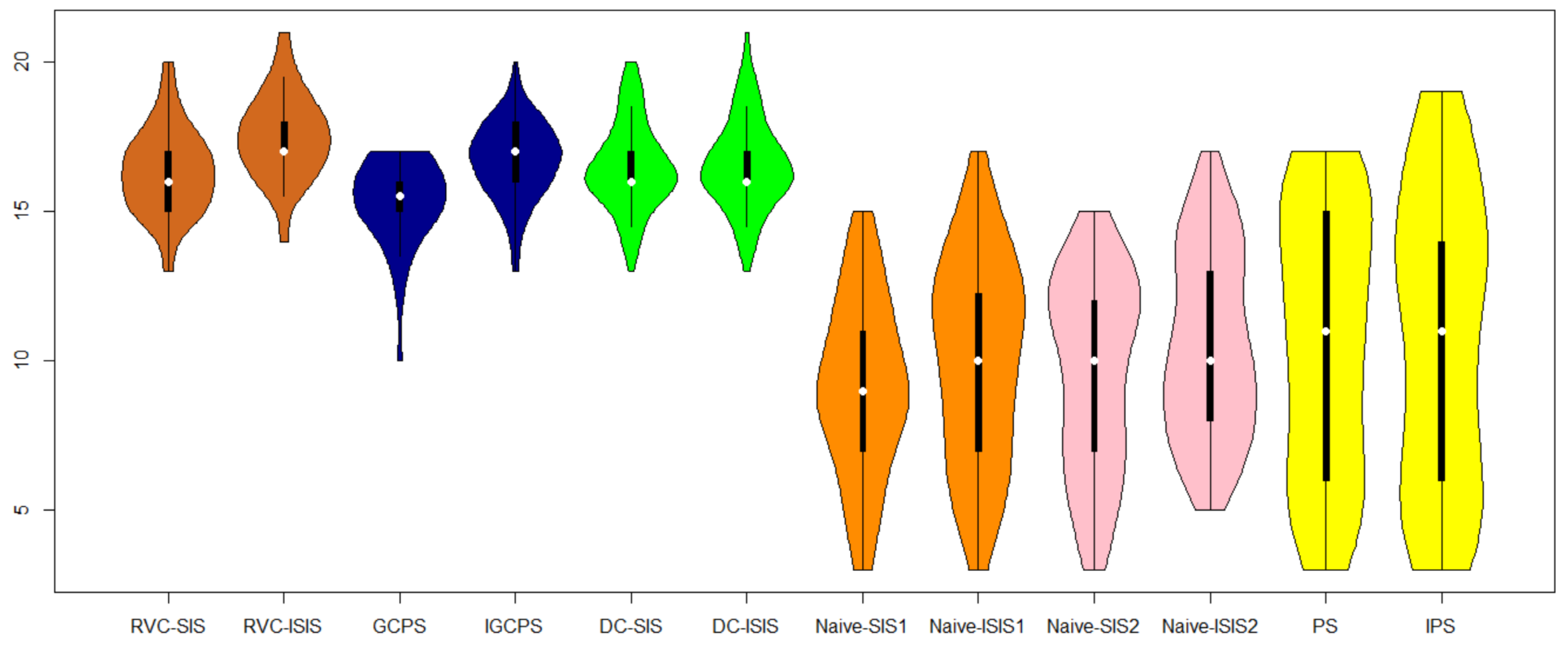
M: The minimum model size to include all active predictors. In other words, M represents the largest rank of the true predictors: $M={max}_{j\in \mathcal{A}}{R}_j$, where $\mathcal{A}$ is the true model. We report the $5\%,25\%,50\%,75\%$, and $95\%$ quantiles of M from 1000 repetitions.

(iii)

$P_j$: The proportion of important predictor $X_j,j\in \mathcal{A}$ being selected for a given model size $[n/log(n\left)\right]$ in the 1000 replications.

(iv)

$P_a$: The proportion of all active predictors being selected into the submodel with size $[n/log(n\left)\right]$ over 1000 simulations.

Example 1.

Following Li et al. [3], we consider a linear model with multivariate responses as follows.

$$\begin{array}{ccc}\hfill Y_1& =& {\beta }_{11}{X}_1+{\beta }_{12}{X}_2+\cdots +{\beta }_{15}{X}_5+{\epsilon }_1,\hfill \\ \hfill ⋮& & ⋮\hfill \\ \hfill Y_{q_n}& =& {\beta }_{q_n,1}{X}_1+{\beta }_{q_n,2}{X}_2+\cdots +{\beta }_{q_n,5}{X}_5+{\epsilon }_{q_n}.\hfill \end{array}$$

The dimension of the response is $q_n=\left[n^{\alpha }\right],\alpha \sim U(0.2,0.9)$. The truly active predictors set is $\mathcal{M}=\{X_1,\dots ,X_5\}$. $\mathbf{X}={(X_1,\dots ,X_p)}^{\top }$ is drawn from a multivariate normal distribution $\mathcal{N}({\mathit{0}}_{p\times 1},\mathsf{\Sigma })$, where Σ is a $p\times p$ covariance matrix with elements ${\sigma }_{ij}=0.8^{|i-j|}$. The nonzero coefficient is given by ${\beta }_{kj}={(-1)}^{W_{kj}}(log\left(\sqrt{n}\right)+|Z_{kj}\left|\right),k=1,\dots ,q_n,j=1,\dots ,5,$ where $W_{kj}$ is a binary random variable with $Pr(W_{kj}=1)=0.6$ and $Z_{kj}\sim \mathcal{N}(0,1)$. The random error term ${\epsilon }_k$ follows the standard normal distribution $\mathcal{N}(0,1)$.

Example 2.

We apply the screening procedures to the additive model when the components of the multivariate response are strongly correlated:

$$\begin{array}{ccc}\hfill Y_1& =& 5f_1\left(X_1\right)+8f_2\left(X_2\right)+4f_3\left(X_3\right)+6f_4\left(X_4\right)+{\epsilon }_1,\hfill \\ \hfill Y_2& =& 4f_1\left(X_1\right)+6f_2\left(X_2\right)+5f_3\left(X_3\right)+8f_4\left(X_4\right)+{\epsilon }_2,\hfill \\ \hfill Y_3& =& 6f_1\left(X_1\right)+4f_2\left(X_2\right)+3f_3\left(X_3\right)+5f_4\left(X_4\right)+{\epsilon }_3,\hfill \end{array}$$

with

$$f_1\left(x\right)=exp\left(sin\left(\pi x\right)\right),f_2\left(x\right)=exp\left(x\right){(2x-1)}^2,f_3\left(x\right)={\displaystyle \frac{sin\left(2\pi x\right)}{2-sin\left(2\pi x\right)}}$$

and

$$f_4\left(x\right)=0.1sin\left(2\pi x\right)+0.2cos\left(2\pi x\right)+0.3{sin}^2\left(2\pi x\right)+0.4{cos}^3\left(2\pi x\right)+0.5{sin}^3\left(2\pi x\right).$$

The predictor $\mathbf{X}={(X_1,\dots ,X_p)}^{\top }$ is generated by

$$X_j={\displaystyle \frac{W_j+U}{2}},j=1,\dots ,p,$$

where $W_1,\dots ,W_p$ and U are i.i.d. U(0,1). The truly active predictors set is $\mathcal{M}=\{X_1,\dots ,X_4\}$. The random error term ${\epsilon }_k$ is from the standard normal distribution $\mathcal{N}(0,1)$.

Example 3.

The following model is taken from Fan and Lv [1] and Li et al. [3].

$$\begin{array}{ccc}\hfill Y_1& =& 5X_1+5X_2+5X_3-15X_4\sqrt{0.5}+{\epsilon }_1,\hfill \\ \hfill Y_2& =& 4X_1+6X_2+8X_3-18X_4\sqrt{0.5}+{\epsilon }_2,\hfill \\ \hfill Y_3& =& 5X_1+4X_2+6X_3-15X_4\sqrt{0.5}+{\epsilon }_3.\hfill \end{array}$$

$\mathbf{X}={(X_1,\dots ,X_p)}^{\top }$ follows a multivariate normal distribution $\mathcal{N}(0_{p\times 1},\mathsf{\Sigma })$. The covariance matrix Σ satisfies ${\sigma }_{11}=\dots ={\sigma }_{pp}=1$ and the off-diagonal elements ${\sigma }_{ij}=0.5,i\ne j$, except for ${\sigma }_{4j}={\sigma }_{j4}=\sqrt{0.5},j\ne 4$. The random error term ${\epsilon }_k$ follows a standard normal distribution $\mathcal{N}(0,1)$. The set of truly active predictors is $\mathcal{M}=\{X_1,\dots ,X_4\}$.

Example 4.

We adopt the simulation model in [1,3] as follows.

$$\begin{array}{ccc}\hfill Y_1& =& 5X_1+5X_2+5X_3-15X_4\sqrt{0.5}+1.25X_5+{\epsilon }_1,\hfill \\ \hfill Y_2& =& 4X_1+6X_2+8X_3-18X_4\sqrt{0.5}+1.5X_5+{\epsilon }_2,\hfill \\ \hfill Y_3& =& 5X_1+4X_2+6X_3-15X_4\sqrt{0.5}+1.25X_5+{\epsilon }_3.\hfill \end{array}$$

The covariance matrix Σ is the same as in Example 3, except that ${\sigma }_{5j}={\sigma }_{j5}=0,j\ne 5$. $X_5$ is uncorrelated with any $X_j,j\ne 5$. The random error term ${\epsilon }_k$ is from the standard normal distribution $\mathcal{N}(0,1)$.

In Example 1, the model is linear, and the response is multivariate. All methods perform well under this scenario, as shown in

Table 1. The average rank $R_j$ of the true predictor $X_j$ for Examples 1–4.

	Method	${\mathit{R}}_{\mathbf{1}}$	${\mathit{R}}_{\mathbf{2}}$	${\mathit{R}}_{\mathbf{3}}$	${\mathit{R}}_{\mathbf{4}}$	${\mathit{R}}_{\mathbf{5}}$
Example 1	Naive-SIS1	4.108	2.48	2.002	2.488	4.056
	Naive-ISIS1	3.856	2.742	2.202	2.342	3.878
	Naive-SIS2	3.71	2.726	2.408	2.722	3.634
	Naive-ISIS2	4.236	3.056	2.408	2.546	2.886
	PS	2.94	2.998	2.99	2.988	3.084
	IPS	3.656	1.016	1.986	3.258	3.798
	DC-SIS	4.53	2.442	1.862	2.464	4.154
	DC-ISIS	4.38	2.347	2.036	2.898	3.956
	GCPS	4.653	2.462	1.362	2.474	4.468
	IGCPS	4.038	2.847	1.362	2.998	4.854
	RVC-SIS	4.156	2.45	1.898	2.494	4.114
	RVC-ISIS	3.832	2.55	2.134	2.256	4.234
Example 2	Naive-SIS1	1006.022	617.534	1709.544	1774.618	-
	Naive-ISIS1	927.04	465.648	107.872	48.554	-
	Naive-SIS2	1078.528	654.678	1737.142	1800.202	-
	Naive-ISIS2	1032.746	509.788	149.616	41.562	-
	PS	1076.362	865.076	734.618	570.108	-
	IPS	1000.356	156.824	9.482	5.864	-
	DC-SIS	125.704	385.02	2.012	1	-
	DC-ISIS	19.254	14.596	2.316	1	-
	GCPS	1.035	677.842	345.654	887.356	-
	IGCPS	1.035	28.647	77.336	96.256	-
	RVC-SIS	8.618	8.12	2.232	1	-
	RVC-ISIS	7.756	4.61	2.536	1	-
Example 3	Naive-SIS1	2.746	2.248	1.028	1002.92	-
	Naive-ISIS1	4.232	2.756	1.028	5.376	-
	Naive-SIS2	2.646	2.358	1.052	1003.12	-
	Naive-ISIS2	3.836	3.112	1.052	5.332	-
	PS	1.556	2.86	1.584	1014.08	-
	IPS	1.556	3.948	1.596	5.386	-
	DC-SIS	2.706	2.284	1.028	982.866	-
	DC-ISIS	4.112	2.878	1.028	5	-
	GCPS	2.732	2.342	1.126	856.562	-
	IGCPS	4.126	2.964	1.126	5.051	-
	RVC-SIS	2.734	2.236	1.032	965.084	-
	RVC-ISIS	4.216	2.758	1.032	5	-
Example 4	Naive-SIS1	2.908	2.306	1.026	1010.838	12.572
	Naive-ISIS1	4.208	2.806	1.026	41.296	6.024
	Naive-SIS2	2.668	2.452	1.036	1011.006	12.306
	Naive-ISIS2	3.796	3.224	1.036	56.808	6.044
	PS	1.552	2.862	1.586	977.962	33.456
	IPS	1.552	3.904	1.586	72.238	5.638
	DC-SIS	2.894	2.316	1.032	968.662	22.386
	DC-ISIS	4.068	2.926	1.032	3.000	6.016
	GCPS	2.825	2.212	1.262	1126.124	36.746
	IGCPS	4.534	2.647	1.262	3.898	8.956
	RVC-SIS	3.054	2.264	1.044	989.44	22.552
	RVC-ISIS	4.134	2.838	1.044	3.000	6.106

NOTE: “-” denotes that there is no corresponding content because of the difference in $\mathcal{M}$.

,

Table 2. The selecting rate $P_j$ of the true predictors and $P_a$ for Examples 1–4.

	Method	${\mathit{P}}_{\mathbf{1}}$	${\mathit{P}}_{\mathbf{2}}$	${\mathit{P}}_{\mathbf{3}}$	${\mathit{P}}_{\mathbf{4}}$	${\mathit{P}}_{\mathbf{5}}$	${\mathit{P}}_{\mathit{a}}$
Example 1	Naive-SIS1	1	1	1	1	1	1
	Naive-ISIS1	1	1	1	1	1	1
	Naive-SIS2	1	1	1	1	1	1
	Naive-ISIS2	1	1	1	1	1	1
	PS	1	1	1	1	1	1
	IPS	1	1	1	1	1	1
	DC-SIS	1	1	1	1	1	1
	DC-ISIS	1	1	1	1	1	1
	GCPS	1	1	1	1	1	1
	IGCPS	1	1	1	1	1	1
	RVC-SIS	1	1	1	1	1	1
	RVC-ISIS	1	1	1	1	1	1
Example 2	Naive-SIS1	0.026	0.168	0	0	-	0
	Naive-ISIS1	0.054	0.234	0.798	0.916	-	0.015
	Naive-SIS2	0.028	0.176	0	0	-	0
	Naive-ISIS2	0.055	0.220	0.702	0.916	-	0.02
	PS	0	0.070	0.110	0.130	-	0
	IPS	0.022	$0.752$	1	1	-	0.016
	DC-SIS	0.628	0.268	1	1	-	0.158
	DC-ISIS	0.986	0.998	1	1	-	0.984
	GCPS	1	0.156	0.278	0.002	-	0
	IGCPS	1	0.996	0.883	0.824	-	0.648
	RVC-SIS	0.964	0.982	1	1	-	0.966
	RVC-ISIS	0.988	0.996	1	1	-	0.986
Example 3	Naive-SIS1	1	1	1	0	-	0
	Naive-ISIS1	1	1	1	1	-	1
	Naive-SIS2	1	1	1	0	-	0
	Naive-ISIS2	1	1	1	1	-	1
	PS	1	1	1	0	-	0
	IPS	1	1	1	1	-	1
	DC-SIS	1	1	1	0	-	0
	DC-ISIS	1	1	1	1	-	1
	GCPS	1	1	1	0	-	0
	IGCPS	1	1	1	1	-	1
	RVC-SIS	1	1	1	0	-	0
	RVC-ISIS	1	1	1	1	-	1
Example 4	Naive-SIS1	1	1	1	0	1	0
	Naive-ISIS1	1	1	1	1	1	1
	Naive-SIS2	1	1	1	0	1	0
	Naive-ISIS2	1	1	1	1	1	1
	PS	1	1	1	0	1	0
	IPS	1	1	1	1	1	1
	DC-SIS	1	1	1	0	1	0
	DC-ISIS	1	1	1	1	1	1
	GCPS	1	1	1	0	1	0
	IGCPS	1	1	1	1	1	1
	RVC-SIS	1	1	1	0	1	0
	RVC-ISIS	1	1	1	1	1	1

and

Table 3. The quantiles of $M={max}_{j\in \mathcal{A}}{R}_j$ for Examples 1–4.

	Method	$\mathbf{5}\mathbf{\%}$	$\mathbf{25}\mathbf{\%}$	$\mathbf{50}\mathbf{\%}$	$\mathbf{75}\mathbf{\%}$	$\mathbf{95}\mathbf{\%}$
Example 1	Naive-SIS1	5	5	5	5	6
	Naive-ISIS1	5	5	5	5	6
	Naive-SIS2	5	5	5	5	6
	Naive-ISIS2	5	5	5	5	6
	PS	5	5	5	5	5
	IPS	5	5	5	5	5
	DC-SIS	5	5	5	5	5
	DC-ISIS	5	5	5	5	5
	GCPS	5	5	5	5	5
	IGCPS	5	5	5	5	5
	RVC-SIS	5	5	5	5	6
	RVC-ISIS	5	5	5	5	6
Example 2	Naive-SIS1	1668.45	1990.75	1969	1994	2000
	Naive-ISIS1	277.9	669	1015	1407.25	1887.05
	Naive-SIS2	1713.4	1913	1975	1995	2000
	Naive-ISIS2	261.25	724.95	1069	1466.5	1846.1
	PS	811.95	1215.25	1488.5	1739.25	1957.15
	IPS	122	512.75	982	1476.5	1940.4
	DC-SIS	22.95	122.75	315.5	653.5	1317.2
	DC-ISIS	5	5	9	12	40.1
	GCPS	280.56	634.85	948.32	1203.46	1568.12
	IGCPS	20.86	38.95	57.78	286.96	500.85
	RVC-SIS	4	4	4	7	46
	RVC-ISIS	4	4	4	7	38
Example 3	Naive-SIS1	430.65	628.5	887.5	1326.25	1879.55
	Naive-ISIS1	5	5	5	5	5
	Naive-SIS2	444.25	639	903.5	1343.5	1878.15
	Naive-ISIS2	5	5	5	5	5
	PS	458.85	682.75	939	1325.75	1829.3
	IPS	4	4	4	5	5
	DC-SIS	337.75	590	871	1389.25	1828.3
	DC-ISIS	5	5	5	5	5
	GCPS	268.65	457.54	671.88	999.58	1509.98
	IGCPS	5	5	5	5	5
	RVC-SIS	284.65	596.75	880	1299.25	1811.35
	RVC-ISIS	5	5	5	5	5
Example 4	Naive-SIS1	426.8	639.5	903	1394	1840.2
	Naive-ISIS1	6	6	6	6	6
	Naive-SIS2	421.9	641.25	890.5	1368.25	1835.35
	Naive-ISIS2	6	6	6	6	6
	PS	373.85	676.75	935	1253.25	1809.25
	IPS	5	5	5.5	6	7
	DC-SIS	304.9	609.75	922	1324.5	1809.05
	DC-ISIS	6	6	6	6	6
	GCPS	298.25	807.75	1130.42	1628.75	1811.50
	IGCPS	6	6	6	6	6
	RVC-SIS	258.95	572.5	934.5	1424.25	1876.15
	RVC-ISIS	6	6	6	6	6

.

In Example 2, the model is nonlinear. Each component of the multivariate response has the same nonlinear function of the active predictors. The only difference is the corresponding coefficients. It is easy to check, in this example, that the components of the response are strongly correlated. Note that the smaller the rank of a predictor, the easier it is to be selected. Thus, we can conclude from Table 1 that our proposed method RVC-SIS and RVC-ISIS outperforms the remaining ones in terms of the rank of the important predictors. Naive-SIS1, Naive-SIS2, and PS perform badly in selecting the important predictors $X_1$–$X_4$. Naive-ISIS1 and Naive-ISIS2 still fail to detect $X_1$–$X_2$, while IPS still exhibits bad performances in choosing $X_1$ due to the large rank. The rank of active variables $X_2$–$X_4$ in GCPS is too high to be chosen, while the rank of $X_2$ in IGCPS is low enough to be selected. Although DC-SIS behaves badly in selecting $X_2$ in this context, DC-ISIS dramatically improves its performance. From Table 2, we can see that DC-ISIS, RVC-SIS, and RVC-ISIS can pick up $X_1$–$X_4$ with an overwhelming probability. Naive-SIS1, Naive-SIS2, and PS select these predictors with little chance. Naive-ISIS1 and Naive-ISIS2 still fail to detect $X_1$–$X_2$, while IPS cannot identify $X_1$. GCPS selects $X_1$ with overwhelming probability, while IGCPS chooses $X_2$–$X_4$ with a large probability. Table 3 demonstrates that only DC-ISIS, RVC-SIS, and RVC-ISIS include all important predictors $X_1$–$X_4$ with a low M, indicating that the four predictors have a higher priority of being selected by these screening methods and thus are ranked at the top.

In Example 3, it is evident that predictor $X_4$ is marginally uncorrelated with $\mathbf{Y}$ at the population level, but it is important to $\mathbf{Y}$. Table 1 shows that Naive-SIS1, Naive-SIS2, PS, DC-SIS, GCPS, and RVC-SIS consistently identify $X_4$ with a larger rank, while the proposed iterative screening procedures of these methods screen out $X_4$ with a smaller rank. This indicates that the iterative screening procedure can effectively tackle the second challenge that is mentioned at the beginning of Section 3. Table 2 demonstrates that Naive-SIS1, Naive-SIS2, PS, DC-SIS, GCPS, and RVC-SIS select $X_4$ with little probability, while their respective iterative screening procedures can pick it up with an overwhelming probability. It can be seen from Table 3 that the model size of Naive-SIS1, Naive-SIS2, PS, DC-SIS, GCPS, and RVC-SIS is consistently large due to the incapability of identifying $X_4$.

In Example 4, it is worth noting that important predictor $X_4$ is again uncorrelated with the response $\mathbf{Y}$, and $X_5$ has a very small correlation with response $\mathbf{Y}$. In fact, variable $X_5$ has the same proportion of contributions to the response as noise ${\epsilon }_i$ does. Similar conclusions can be drawn from these tables due to the existence of $X_4$. Furthermore, these screening methods have a lower priority of selecting $X_5$ than $X_1$–$X_3$ due to the small contribution of $X_5$ to the response.

5. Application

In order to demonstrate the application of our proposed method, we used yeast cell-cycle gene expression data in Spellman et al. [25] and chromatin immunoprecipitation on chip (CHIP-chip) data from Lee et al. [26]. The yeast cell-cycle gene expression data consist of 542 genes from a factor-based experiment in which 18 mRNA levels are measured every 7 min for 119 min.

The chromatin immunoprecipitation on chip (ChIP-chip) data contain the binding information for 106 transcription factors (TFs), which are related to cell regulation. These two datasets are combined as the yeast cell-cycle dataset available in the R package spls. For further details about this dataset, please refer to Chun and Keles [27].

First, the data are randomly split into a training set of 300 and a test set of 242. We apply all screening methods on the training set to select the active predictors. To obtain the threshold in the screening procedures, we introduce auxiliary variables proposed by Zhu et al. [6]. That is, we independently generate $d=2000$ auxiliary variables $\mathbf{Z}\sim {\mathcal{N}}_d(0,{\mathbf{I}}_d)$ such that $\mathbf{Z}$ is independent of both $\mathbf{Y}$ and $\mathbf{X}$. Consider the $(p+d)$-dimensional vector ${({\mathbf{X}}^{\top },{\mathbf{Z}}^{\top })}^{\top }$ as the predictors and $\mathbf{Y}$ as the response. Then, we calculate $\widehat{{\omega }_j}$ for $j=1,\dots ,p+d$. Note that $\mathbf{Z}$ is truly inactive via artificial construction, and we can define a threshold

$$C_d=\underset{j=p+l\dots ,p+d}{max}\widehat{{\omega }_j}$$

to select the important predictors. We repeated the random data segmentation 100 times to avoid the impact of random segmentation on the results and comparisons.

Note that there are 21 known and experimentally verified TFs related to the cell-cycle process, as stated in Wang et al. [28]. We then compare the number of confirmed TFs selected in the screening procedure mentioned earlier. The results are reported in Figure 1. From this figure, it can be concluded that RVC-ISIS performs best among all screening procedures, and RVC-SIS performs best among the screening procedures except the iterative ones.

Furthermore, we applied the test set to assess the performance of the screening procedures in terms of the mean square error of the predictions, which can be found in Figure 2 and

Table 4. Averaged mean squared errors (AMSEs) of the prediction over 100 random data partitions and the corresponding standard deviations of the screening procedures.

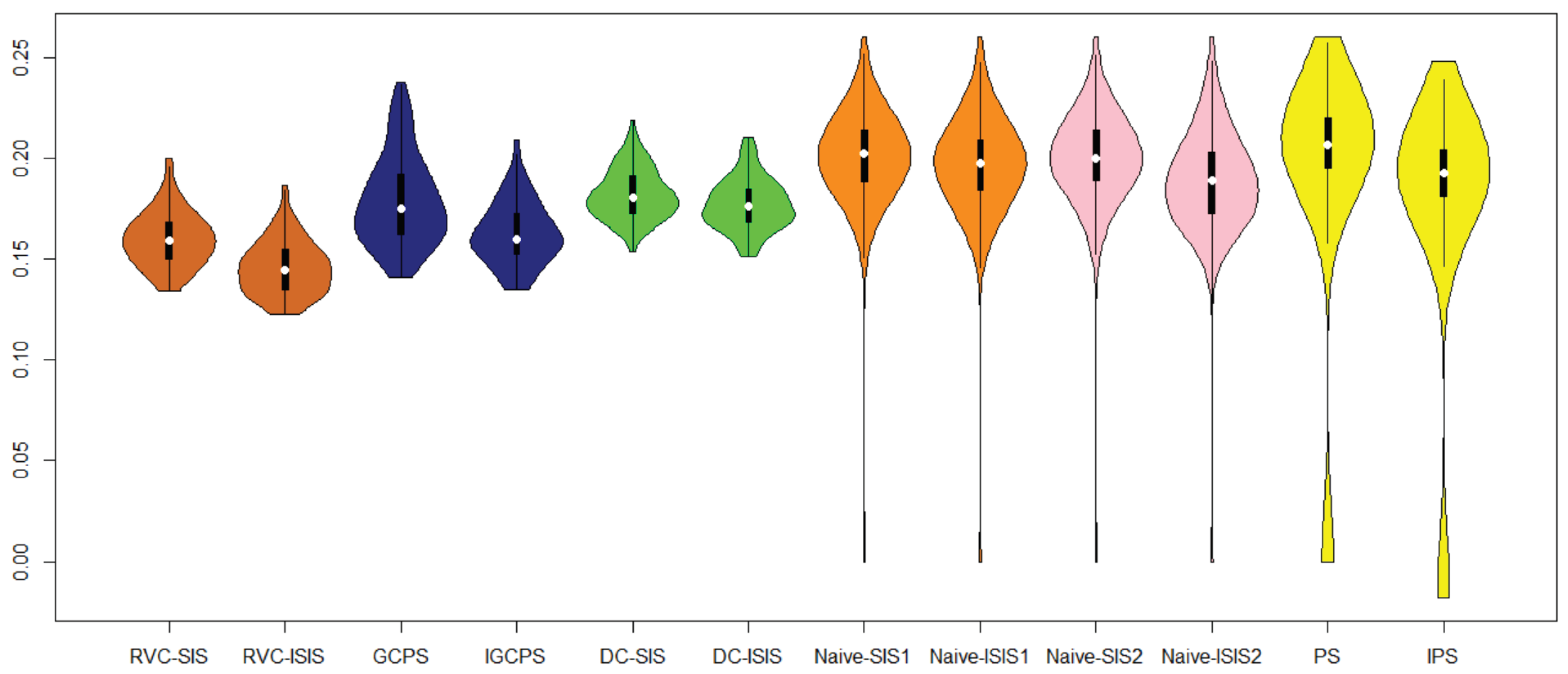
Method	AMSE	Standard Deviation
Naive-SIS1	0.1997	0.0281
Naive-ISIS1	0.1959	0.0286
Naive-SIS2	0.1991	0.0278
Naive-ISIS2	0.1878	0.0288
PS	0.1898	0.0652
IPS	0.1749	0.0604
DC-SIS	0.1822	0.0124
DC-ISIS	0.1772	0.0126
GCPS	0.1668	0.0223
IGCPS	0.1629	0.0221
RVC-SIS	0.1601	0.0136
RVC-ISIS	0.1422	0.0134

. It can be seen that these iterative screening procedures uniformly outperform the original non-iterative screening ones.

6. Discussion

Through extensive simulations and a real data example, we see that the proposed procedure outperforms 58–100% of the existing candidates such as the Naive-SIS1, Naive-ISIS1, Naive-SIS2, Naive-ISIS2, PS and IPS by Li et al. [3], GCPS and IGCPS by Liu et al. (2020) [4], DC-SIS by Li et al. [10], and DC-ISIS by Zhong and Zhu [23]. On average, the proposed method outperforms 79% of existing methods across both linear and nonlinear scenarios. In particular, the proposed method has an enormous advantage in the nonlinear scenarios, with multivariate responses being strongly correlated, like in Example 2.

There exists some limitations in the proposed screening method as well. First, as Muthyala et al. (2024) [29] pointed out, although sure independence screening methods have been proven to be particularly effective in the natural sciences and clinical studies, its widespread adoption has been limited by performance inefficiencies and the challenges posed by its R-based or FORTRAN-based implementation, especially in modern computing environments with massive data. More fast and efficient implementation using new techniques, such as PyTorch 3.12 —based implementations, are necessary for the proposed RVC-SIS and RVC-ISIS algorithms, which is critical for projects like chronic thromboembolic pulmonary hypertension studies [30] with ultrahigh-dimensional multimodal medical data, including radiomics features, genomics data, laboratory omics data, and so on.

Second, this paper only considered the sure independence screening for additive models of continuous multivariates response. However, in clinical practice, such as the pulmonary thromboembolism study, the majority of clinical outcomes is of the binary or survival type. The proposed method and algorithm cannot be directly applied to either scenarios with multivariate, binary, or multilevel categorical outcomes or the scenarios with survival outcomes. However, it is relatively easy to adaptive the proposed RVC-SIS and RVC-ISIS to other types of outcomes using routine methods of related statistical fields.

Last but not the least, we do not investigate the performance of our proposed method for the skewed and heavy-tailed distributed data [31]. Further exploring the interactions between (among) predictors and detecting the corresponding ones is beyond the scope of this paper. These could be interesting topics for future research.

7. Conclusions

This paper investigated a nonparametric screening method for sparse, ultrahigh-dimensional additive models with multivariate responses. We proved that the RVC-SIS exhibits sure screening and ranking consistency properties under certain regularity conditions. In addition, we show, through extensive simulation study, that the proposed RVC-ISIS procedure effectively detects the truly important predictors even in the presence of complex correlations among predictors. The proposed method in this article has great potential for applications in developing nonlinear models with both ultrahigh-dimensional predictors and multivariate responses, especially in the chronic thromboembolic pulmonary hypertension study, where there exist multi-organ linkage responses, such as the right-sided heart failure in hearts, chronic thromboembolic pulmonary hypertension in lungs, and cerebral thrombosis in the brain.

References

- Fan, J.; Lv, J. Sure independence screening for ultrahigh-dimensional feature space. J. R. Stat. Soc. Ser. (Stat. Methodol.) 2008, 70, 849–911. [Google Scholar] [CrossRef]
- Fan, J.; Samworth, R.; Wu, Y. Ultrahigh-dimensional feature selection: Beyond the linear model. J. Mach. Learn. Res. 2009, 10, 2013–2038. [Google Scholar] [PubMed]
- Li, X.; Cheng, G.; Wang, L.; Lai, P.; Song, F. Ultrahigh-dimensional feature screening via projection. Comput. Stats Data Anal. 2017, 114, 88–104. [Google Scholar] [CrossRef]
- Liu, S.; Li, X.; Zhang, J. Ultrahigh-dimensional feature screening for additive model with multivariate response. J. Stat. Comput. Simul. 2020, 90, 775–799. [Google Scholar] [CrossRef]
- Fan, J.; Song, R. Sure independence screening in generalized linear models with NP-dimensionality. Ann. Stat. 2010, 38, 3567–3604. [Google Scholar] [CrossRef]
- Zhu, L.P.; Li, L.; Li, R.; Zhu, L.X. Model-free feature screening for ultrahigh-dimensional data. J. Am. Stat. Assoc. 2011, 106, 1464–1475. [Google Scholar] [CrossRef]
- Fan, J.; Feng, Y.; Song, R. Nonparametric independence screening in sparse ultra-high-dimensional additive models. J. Am. Stat. Assoc. 2011, 106, 544–557. [Google Scholar] [CrossRef]
- Yuan, Y.; Billor, N. Sure independent screening for functional regression model. Commun. Stat.-Simul. Comput. 2024, 1–20. [Google Scholar] [CrossRef]
- Cui, H.; Zou, F.; Ling, L. Feature screening and error variance estimation for ultrahigh-dimensional linear model with measurement errors. Commun. Math. Stat. 2025, 13, 139–171. [Google Scholar] [CrossRef]
- Li, R.; Zhong, W.; Zhu, L. Feature screening via distance correlation learning. J. Am. Stat. Assoc. 2012, 107, 1129–1139. [Google Scholar] [CrossRef]
- Shao, X.; Zhang, J. Martingale difference correlation and its use in high-dimensional variable screening. J. Am. Stat. Assoc. 2014, 109, 1302–1318. [Google Scholar] [CrossRef]
- Cui, H.; Li, R.; Zhong, W. Model-free feature screening for ultrahigh-dimensional discriminant analysis. J. Am. Stat. Assoc. 2015, 110, 630–641. [Google Scholar] [CrossRef]
- Chen, S.; Lu, J. Quantile-Composited feature screening for ultrahigh-dimensional data. Mathematics 2023, 11, 2398. [Google Scholar] [CrossRef]
- Liu, R.; Deng, G.; He, H. Generalized Jaccard feature screening for ultra-high dimensional survival data. AIMS Math. 2024, 9, 27607–27626. [Google Scholar] [CrossRef]
- Sang, Y.; Dang, X. Grouped feature screening for ultrahigh-dimensional classification via Gini distance correlation. J. Multivar. Anal. 2024, 204, 105360. [Google Scholar] [CrossRef]
- Wu, J.; Cui, H. Model-free feature screening based on Hellinger distance for ultrahigh-dimensional data. Stat. Pap. 2024, 65, 5903–5930. [Google Scholar] [CrossRef]
- Zhong, W.; Li, Z.; Guo, W.; Cui, H. Semi-distance correlation and its applications. J. Am. Stat. Assoc. 2024, 119, 2919–2933. [Google Scholar] [CrossRef]
- Tian, Z.; Lai, T.; Zhang, Z. Variation of conditional mean and its application in ultrahigh-dimensional feature screening. Commun. Stat.-Theory Methods 2025, 54, 352–382. [Google Scholar] [CrossRef]
- Li, L.; Ke, C.; Yin, X.; Yu, Z. Generalized martingale difference divergence: Detecting conditional mean independence with applications in variable screening. Comput. Stat. Data Anal. 2023, 180, 107618. [Google Scholar] [CrossRef]
- Liu, L.; Lian, H.; Huang, J. More efficient estimation of multivariate additive models based on tensor decomposition and penalization. computational statistics and data analysis. J. Mach. Learn. Res. 2024, 25, 1–27. [Google Scholar]
- Desai, N.; Baladandayuthapani, V.; Shinohara, R.; Morris, J. Covariance Assisted Multivariate Penalized Additive Regression (CoMPAdRe). J. Comput. Graph. Stat. 2024, 1–10. [Google Scholar] [CrossRef]
- Escoufier, Y. Le traitement des variables vectorielles. Biometrics 1973, 29, 751–760. [Google Scholar] [CrossRef]
- Zhong, W.; Zhu, L. An iterative approach to distance correlation-based sure independence screening. J. Stat. Comput. Simul. 2015, 85, 2331–2345. [Google Scholar] [CrossRef]
- Liu, J.; Li, R.; Wu, R. Feature selection for varying coefficient models with ultrahigh-dimensional covariates. J. Am. Stat. Assoc. 2014, 109, 266–274. [Google Scholar] [CrossRef]
- Spellman, P.T.; Sherlock, G.; Zhang, M.Q.; Iyer, V.R.; Anders, K.; Eisen, M.B.; Brown, P.O.; Botstein, D.; Futcher, B. Comprehensive identification of cell cycle–regulated genes of the yeast Saccharomyces cerevisiae by microarray hybridization. Mol. Biol. Cell 1998, 9, 3273–3297. [Google Scholar] [CrossRef]
- Lee, T.I.; Rinaldi, N.J.; Robert, F.; Odom, D.T.; Bar-Joseph, Z.; Gerber, G.K.; Hannett, N.M.; Harbison, C.T.; Thompson, C.M.; Young, R.A.; et al. Transcriptional regulatory networks in Saccharomyces cerevisiae. Science 2002, 298, 799–804. [Google Scholar] [CrossRef] [PubMed]
- Chun, H.; Keles, S. Sparse partial least squares regression for simultaneous dimension reduction and variable selection. J. R. Stat. Soc. Ser. (Stat. Methodol.) 2010, 72, 3–25. [Google Scholar] [CrossRef]
- Wang, L.; Chen, G.; Li, H. Group SCAD regression analysis for microarray time course gene expression data. Bioinformatics 2007, 23, 1486–1494. [Google Scholar] [CrossRef]
- Muthyala, M.; Sorourifar, F.; Paulson, J.A. TorchSISSO: A PyTorch-based implementation of the sure independence screening and sparsifying operator for efficient and interpretable model discovery. Digit. Chem. Eng. 2024, 13, 100198. [Google Scholar] [CrossRef]
- Xie, W.; Yu, Y.; Huang, Q.; Yan, X.; Yang, Y.; Xiong, C.; Liu, Z.; Wan, J.; Gong, S.; Wang, L.; et al. Epidemiology and management patterns of chronic thromboembolic pulmonary hypertension in China: A systematic literature review and meta-analysis. Chin. Med J. 2025, 138, 1000–1002. [Google Scholar] [CrossRef]
- Song, Y.; Zhou, W.; Zhou, W.X. Large-scale inference of multivariate regression for heavy-tailed and asymmetric data. Stat. Sin. 2023, 33, 1831–1852. [Google Scholar] [CrossRef]
- Serfling, R.J. Approximation Theorems of Mathematical Statistics; John Wiley & Sons: Hoboken, NJ, USA, 1980. [Google Scholar]