An Analytical Solution for the Steady Seepage of Localized Line Leakage in Tunnels

Abstract

This paper proposes an analytical solution for the seepage field when a localized line leakage occurs in a tunnel by accurately considering the boundary conditions at the leakage site, which overcomes the problem of current methods, such as the equivalent method or methods improving on the existing analytical solution for fully drained tunnels, being unable to give an accurate analytical solution. First, the semi-infinite seepage region is converted into a rectangular seepage region using two conformal transformations. Subsequently, in order to accurately consider the boundary conditions at the leakage site, the rectangular seepage region with a discontinuous boundary is divided into three subregions with continuous boundaries, and the water head solution for each subregion is given by using the separated variable method. Finally, the principle of orthogonality of trigonometric functions is specially adopted to construct a non-homogeneous system of equations to solve the unknowns in the analytical solution, and through the inverse transformation of the conformal transformation, an analytical solution for the steady-state seepage field when localized line leakage occurs in a tunnel is obtained. The solution proposed is verified by its satisfactory agreement with the numerical simulation results and existing experimental results, and is much more accurate than the existing analytical solution. In addition, the proposed analytical solution is much less computationally demanding compared to numerical simulations. Finally, the capability of the proposed analytical solution is demonstrated by a parametric analysis of the tunnel burial depth, leakage location, and leakage width, and some meaningful conclusions are drawn.

1. Introduction

Water seepage due to local leakage is a common tunnel defect [1,2]. Three types of leakages (point, line, and surface) correspond to the different levels of damage, with which water leaks through the tunnel lining structure [3]. In Shanghai shield tunnels [4], line leakage is the most common of the three types and more severe than point leakage. Line leakage has a certain continuity and regularity, mainly realized as seam leakage, which mainly appears in construction joints, deformation joints, and longitudinal cracks (mainly in the foot of the arch and the side wall, in the shape of a strip, generally up to tens of meters long). For example, in shield tunnels, line water leakage usually occurs at joints, which could reduce the pore pressure and increase the effective stress in the soil around the tunnels, inducing settlement and disrupting the operation of tunnels [5,6]. In this context, the severity of local line leakage may determine the performance of tunnel linings [7]. Therefore, the prediction and evaluation of line leakage are essential and deserve detailed investigation.

Water leakage in tunnels is a typical tunnel seepage problem which requires the accurate evaluation of seepage volume and attendant pore water pressure. To this end, both numerical and analytical methods have been developed. There are three categories of numerical methods, i.e., homogeneous [8], differential [6], and local [4,9,10] leakage models. These models have been validated and facilitated by finite-difference software but are generally computationally intensive due to the complicated modeling, gridding, and computing procedure. In contrast to the numerical methods, the analytical methods are more straightforward and computationally more efficient but could yield results as accurate as numerical methods. Remarkably, they reflect the influence of multiple factors as explicit functions, enabling the parametric study of the seepage pattern in practice.

Various methods have been employed to derive analytical solutions for tunnel seepage fields under different assumptions [11,12,13,14]. Park et al. [15] propose two different circumferential boundary conditions of a tunnel under zero water pressure or constant total water head. With these two boundary conditions, semi-analytical or analytical solutions for tunnel seepage can be derived by introducing conformal mapping for tunnels without or with grouting rings [16,17,18,19,20,21,22]. However, these analytical solutions are based on the assumption that the tunnel is fully drained and the leakage is distributed globally. Therefore, they cannot be used to accurately solve localized line leakage, which is a common situation in practice. Guo et al. [23] present an approximate solution for groundwater seepage through a line defect into a sewer by Mobius transform and the equivalent perimeter method. Tang et al. [24] present another analytical method for the pore water pressure around a pipe with a line defect and groundwater seepage through the defective pipe. However, this analytical solution is obtained by assuming that the leakage site is a fully drained circle and improving the analytical solution for fully drained tunnels proposed in [17]. This assumption of the leakage boundary is obviously very different from the actual situation, so unsurprisingly, these results deviate significantly from the numerical simulation and experimental results. In summary, the existing analytical solutions for the seepage fields in tunnels with localized water leakage are not exact analytical solutions. There is a big gap between them and the numerical simulation results and experimental results, because they do not accurately consider the boundary conditions of the leakage location, and most of the analytical methods adopt the equivalent method or the method of improving the existing solutions, without a strict derivation process.

This paper proposes an analytical solution for a seepage field when localized line leakage occurs in a tunnel by accurately considering the boundary conditions at the leakage site, which overcomes the problem of current approaches which use the equivalent method, or a method that improves on the existing analytical solution for fully drained tunnels, being unable to give an accurate analytical solution. The proposed solution is validated by comparing it to the numerical simulation results and experimental results. Its accuracy is evaluated in comparison with existing similar approximate methods. Finally, a parametric analysis of the tunnel burial depth, leakage location, and leakage width is carried out to explore the effects of these three parameters on the seepage field and to demonstrate the capability of the proposed analytical solution.

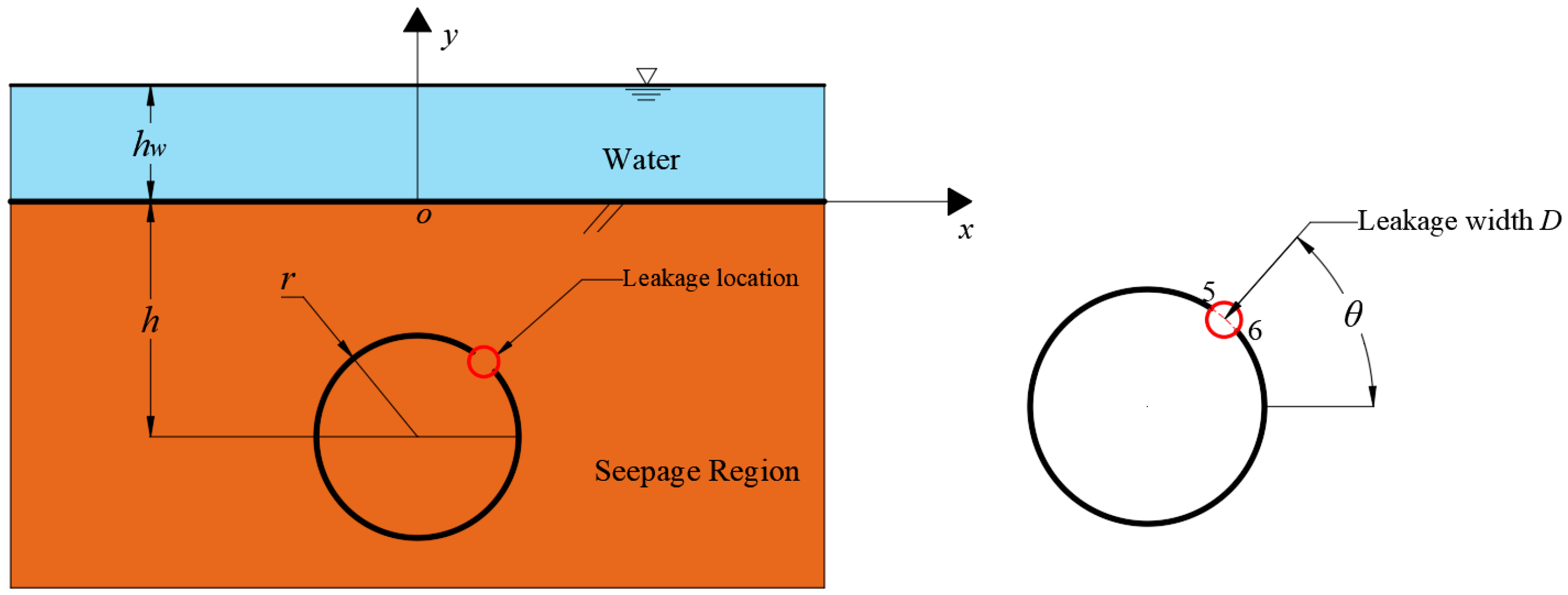
2. Problem Statement

The local line leakage in circular tunnels in semi-infinite saturated soils is usually approximated as a planar seepage problem because the along-tunnel longitudinal dimension of a line leakage is, by definition, much larger than the transversal dimension. Figure 1 shows the planar model for the local line leakage in which the geometrical metrics are as follows: r is the radius of the circular tunnel; h is the distance between the tunnel center and the ground; θ is the azimuthal angle of the leakage center; D is the arc length of the leakage; and points 5 and 6 are the boundaries of the leakage site, i.e., the tunnel leakage site is located between points 5 and 6. By this model, the problem of evaluating local line leakage is described as follows: given the surface water level h_w and the leakage geometry in Figure 1, solve the seepage and the pore pressure by the following governing equation:

$${\displaystyle \frac{{\partial }^{2}H}{\partial x^2}}+{\displaystyle \frac{{\partial }^{2}H}{\partial y^2}}=0$$

(1)

where H is the total hydraulic head. To yield an analytical solution to this equation, it must be solved with the following boundary conditions:

• At the infinite distance from the tunnel center, an impermeable boundary is assumed, indicating that the portion of the tunnel lining outside the water leakage location is impermeable;
• The leakage location is regarded as the zero pore pressure boundary. Because the water leakage fissure is usually small, it is reasonable to utilize the hydraulic head of the leakage location as the elevation head at the leakage center, i.e., h₂ = −h + rsinθ.

Other hypotheses for the analytical solution include the following: the soil is homogeneous and isotropic with a constant permeability coefficient; the groundwater seepage is steady-state; the groundwater level is fixed; and the seepage in the soil follows Darcy’s law.

3. Analytical Solution

Due to the complex geometry of the computational region inherent in the problem of local line leakage (Figure 1), the analytical solution can neither be solved by the mirror method [11] due to the boundary conditions, nor by any direct applications of the conformal mapping method. Consequently, the conformal mapping method and the separation-of-variables method are jointly utilized in this study to solve the seepage field in the problem specified. More specifically, the complex computational domain in the z-plane was first mapped onto the ζ-plane by conformal mapping. The complex domain was converted into a whole rectangular computational region. The mapping does not change the corresponding boundary conditions; thus, the boundary conditions of the rectangular regions in the ζ-plane are still discontinuous due to the occurrence of leakage, which violates the requirement for the continuous boundary of the separation-of-variables method and does not allow for an accurate consideration of the leakage boundary. Therefore, to apply this method and to consider accurately the leakage boundary, the whole rectangular region in the ζ-plane was further divided into several subregions and then decomposed into some pseudo subregions with the same geometry but with different continuous boundary conditions. In such a way, the analytical solutions were given on the decomposed pseudo subregions by the separation-of-variables method and then superposed to yield the analytical solution of the rectangular region. Finally, the analytical solutions of the rectangular regions were combined and then inversely conformal-transformed, yielding the analytical solution of the given problem on the z-plane. This joint application of the conformal mapping method and the separation-of-variables method enables an analytical solution to the local line leakage problem.

The innovation of the proposed method lies in the fact that it overcomes the difficulty of conformal mapping to deal with the boundary conditions at the leakage and to obtain an accurate solution for the seepage field in the case of local leakage [24].

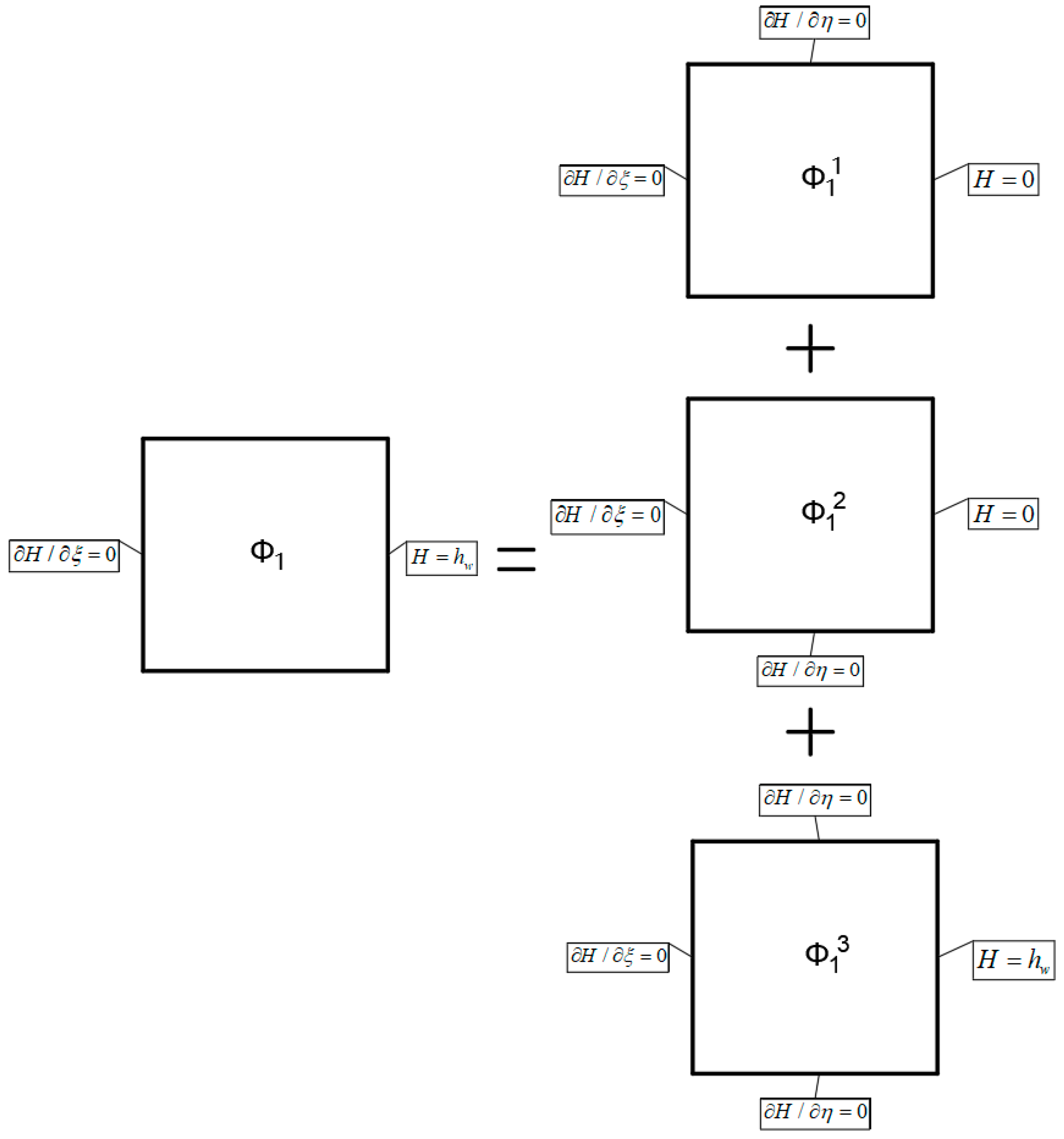
3.1. Conformal Mapping

To carry out the conformal mapping, the problem depicted in Figure 1 is represented by the computational domain in Figure 2a on the z-plane. The computational region is restricted by six nodes (nodes 1–6), where the local leakage is situated between nodes 5 and 6. The mapping function [17,25,26] is utilized to map this region in the z-plane in Figure 2a to the rectangular regions in the ζ-plane in Figure 2b:

$$\zeta =\xi +i\eta =\ln {\displaystyle \frac{z+iA}{z-iA}}$$

(2)

where $A=h{\displaystyle \frac{1-{\alpha }^2}{1+{\alpha }^2}},{\displaystyle \frac{r}{h}}={\displaystyle \frac{2\alpha }{1+{\alpha }^2}},z=x+yi$; i is the imaginary unit; and x-y and ξ-η are the z-plane and ζ-plane coordinates, respectively.

After the above conformal mapping process, the original semi-infinite region is transformed into a whole rectangular seepage region in Figure 2b. However, it is difficult to solve the whole rectangular seepage region in Figure 2b directly by the separation-of-variables method and it is difficult to consider the leakage boundary, because the boundary conditions of the 5–6 boundary are different from those of the 3′–5 and 3–6 boundaries on the same straight line, i.e., the boundary conditions of the 3–3′ boundary are not continuous. Therefore, the entire rectangular seepage region was divided into three rectangular seepage regions to ensure that the boundary conditions of each side of the rectangular seepage region were continuous and that the boundary condition at the seepage site could be accurately taken into account, so as to facilitate the later solution of the analytical formulas for the head of the rectangular seepage regions by the method of separated variables.

It is worth noting that, although the conformal transformation method of converting the seepage region from a concentric circle region to a rectangular region has been applied in many studies [17], these studies did not divide the rectangular seepage region into subregions, which can only consider the continuous boundary conditions of a fully drained tunnel, and cannot consider the case of localized leakage. In contrast, this study divides the rectangular seepage region into subregions, allowing it to accurately consider the boundary conditions at the leakage site and also facilitate the application of the separated variable method to solve the head solution. Finally, the unknowns in the head solution can be solved by the continuity condition between the subregions. Therefore, this conformal transformation combined with the subregion method is a great improvement to the conformal transformation method alone, which provides an accurate solution to the problem of localized water leakage in tunnels, and can also provide solution ideas for other problems with discontinuous boundary conditions.

After two conformal mappings and dividing the ζ-plane rectangular region, the boundary conditions for the three rectangular regions in the ζ-plane are obtained as follows:

• Region ①: the left boundary (ξ = u₀) is impermeable, i.e., $\partial H/\partial \xi =0$; the right boundary is the surface water head h_w;
• Region ②: the left boundary is assumed to be the elevation head at the leakage center h₂; the right boundary is the surface water head h_w;
• Region ③: the left boundary (ξ = u₀) is impermeable, i.e., $\partial H/\partial \xi =0$; the right boundary is the surface water head h_w.

Finally, throughout the conformal mapping process, points are assumed to have one-to-one correspondence, such as points 1 to 6 in Figure 2a corresponding to points 1 to 6 in Figure 2b. Therefore, the unknown coordinate values of points 1 to 6 in Figure 2b can be obtained according to the coordinate values of points 1 to 6 in Figure 2a combined with the conformal mapping formula Equation (2), and the specific unknown coordinate values are as follows:

$$u_0=\ln \alpha$$

(3)

$$v_1=\mathrm{Im}(\ln {\displaystyle \frac{r\cos (\theta -\frac{D}{2r})+(-h+r\sin (\theta -\frac{D}{2r}))i+Ai}{r\cos (\theta -\frac{D}{2r})+(-h+r\sin (\theta -\frac{D}{2r}))i-Ai}})$$

(4)

$$v_2=\mathrm{Im}(\ln {\displaystyle \frac{r\cos (\theta +\frac{D}{2r})+(-h+r\sin (\theta +\frac{D}{2r}))i+Ai}{r\cos (\theta +\frac{D}{2r})+(-h+r\sin (\theta +\frac{D}{2r}))i-Ai}})$$

(5)

3.2. Analytical Solutions for the Seepage Fields

According to Darcy’s law, the seepage in each rectangular region in the ζ-plane is governed by the Laplace equation (Equation (1)). After the conformal mapping, this governing equation is expressed as the mapped equations in three rectangular regions:

$${\displaystyle \frac{{\partial }^2{H}_i}{\partial {\xi }^2}}+{\displaystyle \frac{{\partial }^2{H}_i}{\partial {\eta }^2}}=0;i=1,2,3$$

(6)

where H₁, H_2, and H₃ are the total hydraulic heads of the three subregions, respectively. The continuity condition between these subregions requires the following:

$$\left\{\begin{array}{l}{H}_1{|}_{\eta =v_2}=H_2{|}_{\eta =v_2}\\ {\displaystyle \frac{\partial H_1}{\partial \eta }}{|}_{\eta =v_2}={\displaystyle \frac{\partial H_2}{\partial \eta }}{|}_{\eta =v_2}\end{array}\right.,\left\{\begin{array}{l}{H}_2{|}_{\eta =v_1}=H_3{|}_{\eta =v_1}\\ {\displaystyle \frac{\partial H_2}{\partial \eta }}{|}_{\eta =v_1}={\displaystyle \frac{\partial H_3}{\partial \eta }}{|}_{\eta =v_1}\end{array}\right.,\left\{\begin{array}{l}{H}_1{|}_{\eta =2\pi }=H_3{|}_{\eta =0}\\ {\displaystyle \frac{\partial H_1}{\partial \eta }}{|}_{\eta =2\pi }={\displaystyle \frac{\partial H_3}{\partial \eta }}{|}_{\eta =0}\end{array}\right.$$

(7)

The next step is to apply the separated variable method to solve Equation (6) to obtain the analytical solution of the water head in each region. However, it is worth noting that Regions ①, ②, and ③ do not have homogeneous boundary conditions on the opposite side, so all of them cannot be solved directly by applying the method of separated variables. Therefore, their boundary conditions need to be processed and homogeneous boundaries used in order to apply the separation-of-variables method to solve the analytical solution of the water head.

The most common way to change the non-homogeneous boundary conditions into homogeneous boundaries is the superposition method, which is based on the following ideas [27]:

Firstly, the region is decomposed into several pseudo subregions with opposite sides of homogeneous boundaries. Subsequently, these pseudo subregions are solved by the method of separating variables to obtain the analytical solutions of the water head of each pseudo subregion. Finally, they are superimposed to act as the analytical solution of the water head of the original region.

We take the rectangular Region ① as an example to illustrate the decomposition and superposition of the pseudo subregions. Based on the superposition principle, Region ① is decomposed into the pseudo subregions ${\Phi }_1^1$, ${\Phi }_1^2$, and ${\Phi }_1^3$ with different continuous boundary conditions:

$${\Phi }_1={\Phi }_1^1+{\Phi }_1^2+{\Phi }_1^3$$

(8)

The specific boundary condition superimposition process is shown in Figure 3. For the pseudo subregion ${\Phi }_1^1$, the left and upper boundaries are impermeable, while the hydraulic head at its right boundary is 0. The pseudo subregion ${\Phi }_1^2$ has impermeable left and lower boundaries but a zero hydraulic head at the right boundary. ${\Phi }_1^3$ indicates that the left boundary of Region ① is an impermeable boundary. Its upper and lower boundaries are impermeable, and the hydraulic head at the right boundary is h_w. With these boundary conditions, the total hydraulic head for each pseudo subregion is derived by the separation-of-variables method [28,29] as:

$$H_1^1\left(\xi ,\eta \right)={\displaystyle \sum _{m=1}^{\infty }{A}_m\cosh k_m(\eta -2\pi )\sin k_m\xi }$$

(9)

$$H_1^2\left(\xi ,\eta \right)={\displaystyle \sum _{m=1}^{\infty }{B}_m\cosh k_m(\eta -v_2)\sin k_m\xi }$$

(10)

$$H_1^3\left(\xi ,\eta \right)=h_w$$

(11)

where A_m and B_m are the parameters to be determined, and k_m = (2m − 1)π/2u₀, m = 1, 2, 3…. Accordingly, the total hydraulic head solution for Region ① is the sum of the total hydraulic heads of the three subregions:

$$H_1\left(\xi ,\eta \right)=h_w+{\displaystyle \sum _{m=1}^{\infty }[A_m\cosh k_m(\eta -2\pi )+B_m\cosh k_m(\eta -v_2)]\sin k_m\xi }$$

(12)

By following a similar procedure, the total hydraulic head solutions for Region ② and Region ③ are derived as:

$$H_2\left(\xi ,\eta \right)=h_w-{\displaystyle \frac{h_w-h_2}{u_0}}\xi +{\displaystyle \sum _{n=1}^{\infty }(C_n\cosh k_n(\eta -v_2)+D_n\cosh k_n(\eta -v_1))\sin k_n\xi }$$

(13)

$$H_3\left(\xi ,\eta \right)=h_w+{\displaystyle \sum _{p=1}^{\infty }[E_p\cosh k_p\eta +F_p\cosh k_p(\eta -v_1)]\sin k_p\xi }$$

(14)

where C_n, D_n, E_p, and F_p are the parameters to be determined, and k_n = nπ/u₀, k_p = (2p − 1)π/2u₀, n, p = 1, 2, 3….

By substituting the total hydraulic head solutions for the three regions into the continuity condition between regions (Equation (7)), the following equations are yielded for determining the parameters A_m, B_m, C_n, D_n, E_p, and F_p:

$$\begin{array}{l}{\displaystyle \sum _{m=1}^{\infty }[A_m\cosh k_m(v_2-2\pi )+B_m]\sin k_m\xi }=\\ -{\displaystyle \frac{h_w-h_2}{u_0}}\xi +{\displaystyle \sum _{n=1}^{\infty }(C_n+D_n\cosh k_n(v_2-v_1))\sin k_n\xi }\end{array}$$

(15)

$${\displaystyle \sum _{m=1}^{\infty }{A}_m{k}_m\sinh k_m(v_2-2\pi )\sin k_m\xi }={\displaystyle \sum _{n=1}^{\infty }{D}_n{k}_n\sinh k_n(v_2-v_1)\sin k_n\xi }$$

(16)

$${\displaystyle \sum _{p=1}^{\infty }[E_p\cosh k_p{v}_1+F_p]\sin k_p\xi }=-{\displaystyle \frac{h_w-h_2}{u_0}}\xi +{\displaystyle \sum _{n=1}^{\infty }(C_n\cosh k_n(v_1-v_2)+D_n)\sin k_n\xi }$$

(17)

$${\displaystyle \sum _{p=1}^{\infty }{E}_p{k}_p\sinh k_p{v}_1\sin k_p\xi }={\displaystyle \sum _{n=1}^{\infty }{C}_n{k}_n\sinh k_n(v_1-v_2)\sin k_n\xi }$$

(18)

$${\displaystyle \sum _{m=1}^{\infty }[A_m+B_m\cosh k_m(2\pi -v_2)]\sin k_m\xi }={\displaystyle \sum _{p=1}^{\infty }[E_p+F_p\cosh k_p{v}_1]\sin k_p\xi }$$

(19)

$${\displaystyle \sum _{m=1}^{\infty }{B}_m{k}_m\sinh k_m(2\pi -v_2)\sin k_m\xi }=-{\displaystyle \sum _{p=1}^{\infty }{F}_p{k}_p\sinh k_p{v}_1\sin k_p\xi }$$

(20)

By multiplying both sides of Equations (15)–(20) by sink_nξ, sink_mξ, sink_nξ, sink_pξ, sink_pξ, and sink_pξ and integrating over the interval [u₀,0], respectively, the following equations are yielded:

$$\begin{array}{r}-{\displaystyle \sum _{m=1}^{\infty }[A_m\cosh k_m(v_2-2\pi )+B_m]\sin k_m{u}_0\cos k_n{u}_0\frac{k_n}{k_m^2-k_n^2}}=\\ -{\displaystyle \frac{h_w-h_2}{k_n}}\cos k_n{u}_0-{\displaystyle \frac{u_0}{2}}(C_n+D_n\cosh k_n(v_2-v_1))\end{array}$$

(21)

$$-{\displaystyle \frac{u_0}{2}}{A}_m{k}_m\sinh k_m(v_2-2\pi )=-{\displaystyle \sum _{n=1}^{\infty }{D}_n{k}_n\sinh k_n(v_2-v_1)\sin k_m{u}_0\cos k_n{u}_0\frac{k_n}{k_m^2-k_n^2}}$$

(22)

$$\begin{array}{l}-{\displaystyle \sum _{p=1}^{\infty }[E_p\cosh k_p{v}_1+F_p]\sin k_p{u}_0\cos k_n{u}_0\frac{k_n}{k_p^2-k_n^2}}=\\ -{\displaystyle \frac{h_w-h_2}{k_n}}\cos k_n{u}_0-{\displaystyle \frac{u_0}{2}}(C_n\cosh k_n(v_1-v_2)+D_n)\end{array}$$

(23)

$$-{\displaystyle \frac{u_0}{2}}{E}_p{k}_p\sinh k_p{v}_1=-{\displaystyle \sum _{n=1}^{\infty }{C}_n{k}_n\sinh k_n(v_1-v_2)\sin k_p{u}_0\cos k_n{u}_0\frac{k_n}{k_p^2-k_n^2}}$$

(24)

$$-{\displaystyle \frac{u_0}{2}}[A_m+B_m\cosh k_m(2\pi -v_2)]=-{\displaystyle \frac{u_0}{2}}[E_p+F_p\cosh k_p{v}_1]$$

(25)

$$-{\displaystyle \frac{u_0}{2}}{B}_m{k}_m\sinh k_m(2\pi -v_2)={\displaystyle \frac{u_0}{2}}{F}_p{k}_p\sinh k_p{v}_1$$

(26)

In the derivation of the above six equations, the orthogonality between trigonometric functions is utilized, e.g., ${\displaystyle {\int }_{u_0}^0\sin k_m\xi \sin k_{m^{\prime }}\xi }\mathrm{d}\xi =\left\{\begin{array}{l}0,m\ne m^{\prime }\\ -{\displaystyle \frac{u_0}{2}},m=m^{\prime }\end{array}\right.$. The application of trigonometric orthogonality ensures that infinite series equations can be written in the form of simple matrices, which facilitates solving them by programming them in programming software, and greatly improves the computational efficiency of the analytical solution.

Equations (21)–(26) act as a linear equation system of the coefficients A_m, B_m, C_n, D_n, E_p, and F_p. To solve this system, the infinite order of m, n, and p must be truncated at the first N order. In this situation, it consists of 6N equations and 6N unknowns and thus could be solved by any numerical method without numerical difficulties. The procedure for constructing and solving this system of linear equations can be found in Appendix A.

By substituting these coefficients into Equations (12)–(14) and carrying out the inverse conformal transformation, the analytical solution of the problem stated, i.e., the total hydraulic head under the z-plane, can be derived as:

$$\begin{array}{l}{H}_1\left(x,y\right)=h_w+{\displaystyle \sum _{m=1}^N{A}_m\cosh k_m[(\arctan \frac{A+y}{x}-\arctan \frac{y-A}{x})-2\pi ]\sin k_m\ln \frac{\sqrt{x^2+{(A+y)}^2}}{\sqrt{x^2+{(y-A)}^2}}}\\ +{\displaystyle \sum _{m=1}^N{B}_m\cosh k_m[(\arctan \frac{A+y}{x}-\arctan \frac{y-A}{x})-v_2]\sin k_m\ln \frac{\sqrt{x^2+{(A+y)}^2}}{\sqrt{x^2+{(y-A)}^2}}}\end{array}$$

(27)

$$\begin{array}{ll}{H}_2\left(x,y\right)& =h_w-{\displaystyle \frac{h_w-h_2}{\ln (\frac{h}{r}-\sqrt{\frac{h^2}{r^r}-1})}}\ln {\displaystyle \frac{\sqrt{x^2+{(A+y)}^2}}{\sqrt{x^2+{(y-A)}^2}}}\\ & +{\displaystyle \sum _{n=1}^N{C}_n\cosh k_n[(\arctan \frac{A+y}{x}-\arctan \frac{y-A}{x})-v_2]\sin k_n}\ln {\displaystyle \frac{\sqrt{x^2+{(A+y)}^2}}{\sqrt{x^2+{(y-A)}^2}}}\\ & +{\displaystyle \sum _{n=1}^N{D}_n\cosh k_n[(\arctan \frac{A+y}{x}-\arctan \frac{y-A}{x})-v_1]\sin k_n\ln \frac{\sqrt{x^2+{(A+y)}^2}}{\sqrt{x^2+{(y-A)}^2}}}\end{array}$$

(28)

$$\begin{array}{c}{H}_3\left(x,y\right)=h_w+{\displaystyle \sum _{p=1}^N{E}_p\cosh k_p(\arctan \frac{A+y}{x}-\arctan \frac{y-A}{x})\sin k_p\ln \frac{\sqrt{x^2+{(A+y)}^2}}{\sqrt{x^2+{(y-A)}^2}}}\\ +{\displaystyle \sum _{p=1}^N{F}_p\cosh k_p[(\arctan \frac{A+y}{x}-\arctan \frac{y-A}{x})-v_1]\sin k_p\ln \frac{\sqrt{x^2+{(A+y)}^2}}{\sqrt{x^2+{(y-A)}^2}}}\end{array}$$

(29)

It is worth noting that although the analytical solution presented in this study is for a seepage field when localized water leakage occurs in a tunnel, this analytical solution can be simplified to the analytical solutions assuming constant head at the tunnel boundary [13,17], as specified below:

Since tunnel leakage sites are generally small in size, this study assumes that the lining sites of the tunnel where no water leakage occurs are impermeable boundaries, and the sites of water leakage are constant head boundaries. Therefore, to simplify the analytical solution of this study to the previous solutions [13,17], which assumed that the tunnel boundary is a constant head, it is only necessary to assume that the tunnel boundary is the only leakage boundary in this study, i.e., only Region ② is retained in Figure 2b.

When only the Region in Figure 2b is retained, the boundary conditions of Region ② are as follows: the left boundary is the constant head boundary h₂ (h₂ here can be selected according to the demand), and the right boundary is the surface water head h_w. The continuity conditions of the Region ② boundary are:

$$\left\{\begin{array}{l}{H_2}^{\prime }{|}_{\eta =2\pi }={H_2}^{\prime }{|}_{\eta =0}\\ {\displaystyle \frac{\partial {H_2}^{\prime }}{\partial \eta }}{|}_{\eta =2\pi }={\displaystyle \frac{\partial {H_2}^{\prime }}{\partial \eta }}{|}_{\eta =0}\end{array}\right.$$

(30)

According to the boundary conditions of Region ② and the continuity conditions, the head solution of Region ② in the ζ-plane can be obtained by using the solving method of this study:

$${H_2}^{\prime }\left(\xi ,\eta \right)=h_w-{\displaystyle \frac{h_w-h_2}{u_0}}\xi$$

(31)

The head solution for Region ② in the z-plane can be obtained after the inverse transformation of the conformal transformation:

$${H_2}^{\prime }\left(x,y\right)=h_w-{\displaystyle \frac{h_w-h_2}{\ln (\frac{h}{r}-\sqrt{\frac{h^2}{r^r}-1})}}\ln {\displaystyle \frac{\sqrt{x^2+{(A+y)}^2}}{\sqrt{x^2+{(y-A)}^2}}}$$

(32)

This solution is consistent with the solutions in papers [13,17] that assume a constant head at the tunnel boundary. Therefore, under the assumption that the leakage occurs throughout the tunnel boundary, this solution can be simplified to the previous analytical solutions in papers [13,17] assuming a constant head at the tunnel boundary.

3.3. Analytical Solution for the Seepage Volume at the Leakage Location

The seepage volume at the leakage location between nodes 5 and 6 at the z-plane is equal to that between lines 5 and 6 in the ζ-plane. According to Equation (13), the hydraulic gradient i between lines 5 and 6 can be obtained as:

$$i=-{\displaystyle \frac{h_w-h_2}{u_0}}+{\displaystyle \sum _{n=1}^N(C_n{k}_n\cosh k_n(\eta -v_2)+D_n{k}_n\cosh k_n(\eta -v_1))\cos k_n{u}_0}$$

(33)

Therefore, the seepage flow is given by:

$$\begin{array}{ll}q& ={\displaystyle {\int }_{v_1}^{v_2}ki}d\eta \\ & =k[-{\displaystyle \frac{h_w-h_2}{u_0}}(v_2-v_1)-{\displaystyle \sum _{n=1}^N{C}_n\sinh k_n(v_1-v_2)\cos k_n{u}_0}\\ & +{\displaystyle \sum _{n=1}^N{D}_n\sinh k_n(v_2-v_1)\cos k_n{u}_0}]\end{array}$$

(34)

which gives the analytical solution of the local leakage seepage volume.

3.4. Analytical Solution for the Pore Water Pressure

According to Equations (27)–(29), the analytical solution for pore water pressure is:

$$p_i\left(x,y\right)=H_i(x,y){\gamma }_w-y{\gamma }_w,i=1,2,3$$

(35)

where ${\gamma }_w$ is the weight of water.

4. Validation of the Proposed Analytical Solution

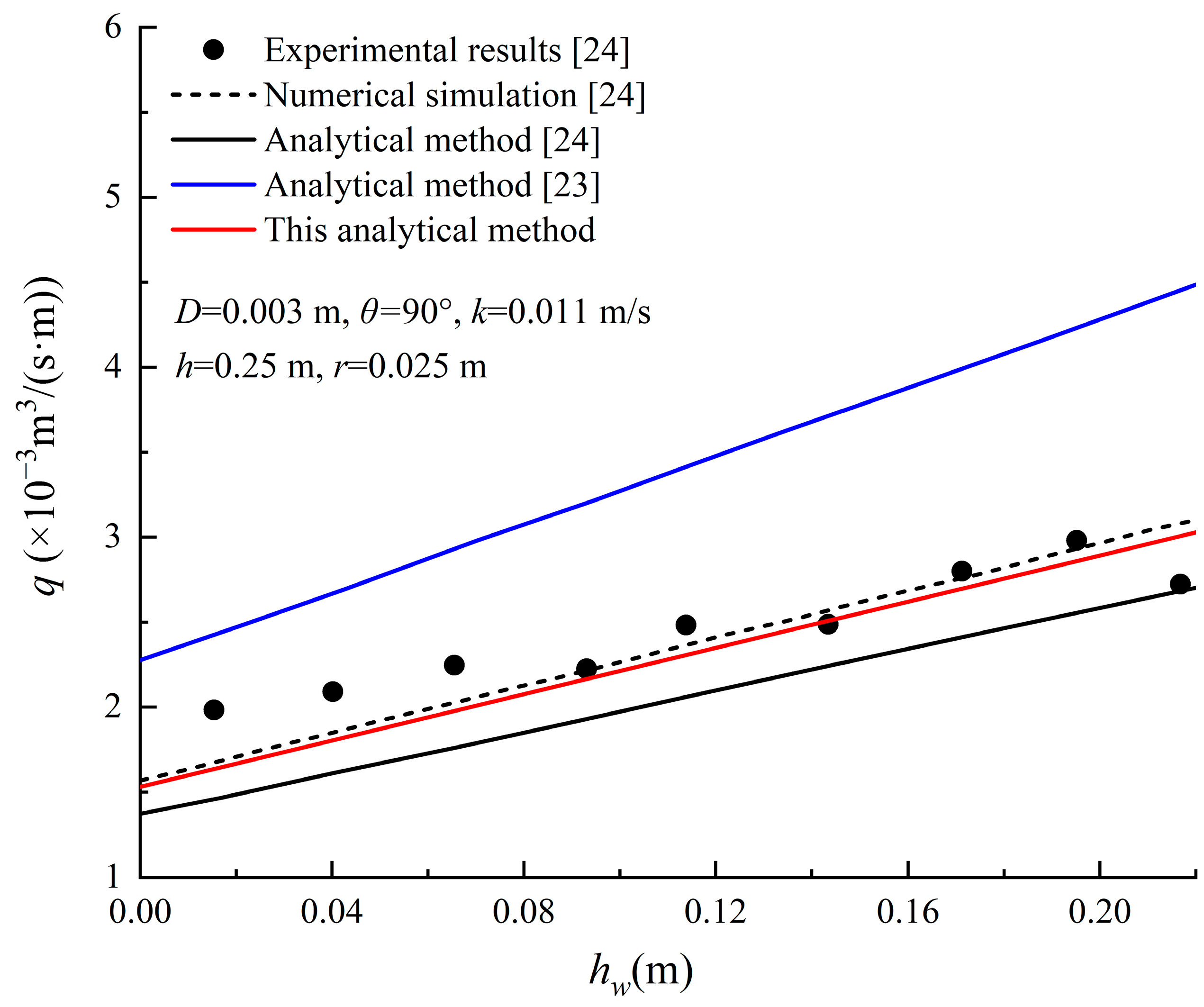
4.1. Seepage Volume

In order to validate the analytical solution proposed, its results were compared to numerical simulation and experimental results in the existing literature. The baseline examples (with various leakage locations) given in Tang et al. [24] were carried out by the proposed analytical solution. The specific model parameters are given in Figure 4 and Figure 5. In the numerical tests, the proposed analytical solution converged when N ≥ 100, which was utilized throughout all the sequential calculations. When N = 100, the analytical solution takes less than 1 s on a computer with Core i7 CPU.

Figure 4 compares the seepage volume calculated by the proposed solution to the numerical simulation results and the test results of Tang et al. [24] with the local leakage at the top of the tunnel. It is evident from Figure 4 that the analytical solution proposed almost overlaps the numerical simulation with a maximum error of less than 2.5%, while the minimum error between the analytical solution of Tang et al. [24] and the numerical simulation results is not less than 12%, which is a large difference. In addition, the proposed analytical solution also agrees well with the experimental data with the maximum error of 17% but mostly within 10%. The errors between the analytical solution of Tang et al. [24] and the experimental data are in the range of 10–25%, which is a large difference, and the approximate solution of Guo et al. [23] has an even larger difference from the numerical simulation results and experimental results. In summary, the proposed analytical solution is far more accurate than the existing analytical solutions.

Figure 5a,b compare the seepage volume calculated by the proposed solution and by numerical simulations (Tang et al. [24]) with various local leakage locations and different leakage widths. The solution of Tang et al. [24] is also presented for reference. It is confirmed that the analytical solution of this paper is almost identical to the numerical solution, and it is much more accurate than the solution given by Tang et al. [21]. It can be seen that the proposed analytical solution can accurately predict the amount of seepage with any leakage locations/widths in the tunnel. Notably, the seepage volume calculation results of this paper’s analytical solution in Figure 5a are almost unchanged, which is because the data in Figure 5a are under the condition of keeping the head difference Δh between the surface water level and the leakage site constant. When Δh is constant, the hydraulic gradient at the leakage site is unchanged, so the seepage volume of the analytical solution in this paper does not change with a change in the leakage location.

The proposed method shows far more accurate predictions than of Tang et al. [24] for a few reasons.

Tang et al. [24] mandates that the site of leakage occurs on a fully permeable circle so that the existing analytical solution (Huangfu et al. [17]) can be utilized. However, this is not the same as the actual leakage, so the results of the solution are clearly inaccurate. In addition, Tang et al. [24] used only the conformal mapping method and were unable to accommodate solutions with different boundary conditions. These accuracies have been partially circumvented in the proposed method. By integrating the conformal mapping with the separation variable method for the partitioned solution, the effects of the leakage site and impermeable lining on the seepage flow field can be accounted for. In this perspective, the proposed method is apparently closer to the numerical simulation results and the experimental results.

4.2. Total Hydraulic Head and Pore Water Pressure

To further validate the analytical solution proposed, the finite-difference software FLAC2D 7.0 was utilized to carry out the numerical simulation of an example with the parameters in

Table 1. Model parameters.

hw (m)	h (m)	r (m)	θ (°)	D (m)	h2 (m)	k (m/s)
15	9	3	0	0.3	−9	1

. This example’s geometry, boundary conditions, and permeability were the same as in the proposed analytical solution. Notably, the permeability coefficient k is only useful when solving for seepage volume, and the effect of different permeability coefficients on seepage volume is simply a multiplicative relationship, so for simplicity of data k = 1 m/s was chosen for this example.

The details of the numerical simulation are as follows: firstly, according to Li et al. [18], it is known that the lateral boundary is at least 9 times the diameter of the tunnel when a numerical simulation of the steady-state seepage field is carried out, so in order to effectively reduce the influence of the simulation domain on the accuracy, the simulation domain of this numerical simulation was determined to be 800 m × 400 m. Subsequently, the geometric model was established by using the finite element software ABAQUS and meshing was carried out, with a focus on encrypting the mesh around the leakage location. Finally, the mesh was imported into FLAC2D 7.0 software, boundary conditions were set, and seepage calculations were performed. The boundary conditions were set as follows: the left, right, and bottom boundaries were fixed horizontally and vertically. The left, right, and lower boundaries were set as permeable boundaries and the pore pressure distributed along the depth was fixed. The ground boundary was free and permeable, converting the surface head to pore pressure applied to the ground. The tunnel lining was set as an impermeable boundary and the water leakage site was set as a zero pore pressure boundary.

Figure 6 and Figure 7 show the comparisons of hydraulic head and water pressure, respectively, between the results given by the analytical solution and the numerical simulation. As observed from the figures, the analytical solution almost coincides with the numerical simulation results, thus validating the proposed analytical solution. However, it is worth noting that the analytical solution in this paper is computationally efficient, and it only takes about 1 s to compute the results using a computer with Core i7 CPU, while the numerical simulation software FLAC2D requires more than 10 s to complete a calculation. In addition, other numerical simulation software, such as ABAQUS 2022 and COMSOL Multiphysics 6.0, require more than 10 s to complete a calculation for the same model. Changing the parameters to recalculate only requires a change the input values in the program without the steps of re-modeling and meshing in numerical software, so the computation time consumed is much shorter than that of the numerical software calculations, which facilitates a large number of parametric analyses.

5. Application of the Proposed Solution: Parametric Study

In this section, the proposed analytical solution is demonstrated by applying it to a parametric study of the local line leakage of a specified tunnel. The varying parameters considered in this section include leakage location, tunnel depth, and leakage width. This parametric study is facilitated only by the proposed analytical solution. As mentioned in the preceding section, the other approximate solutions are not as accurate, while the numerical simulation is computationally far too demanding.

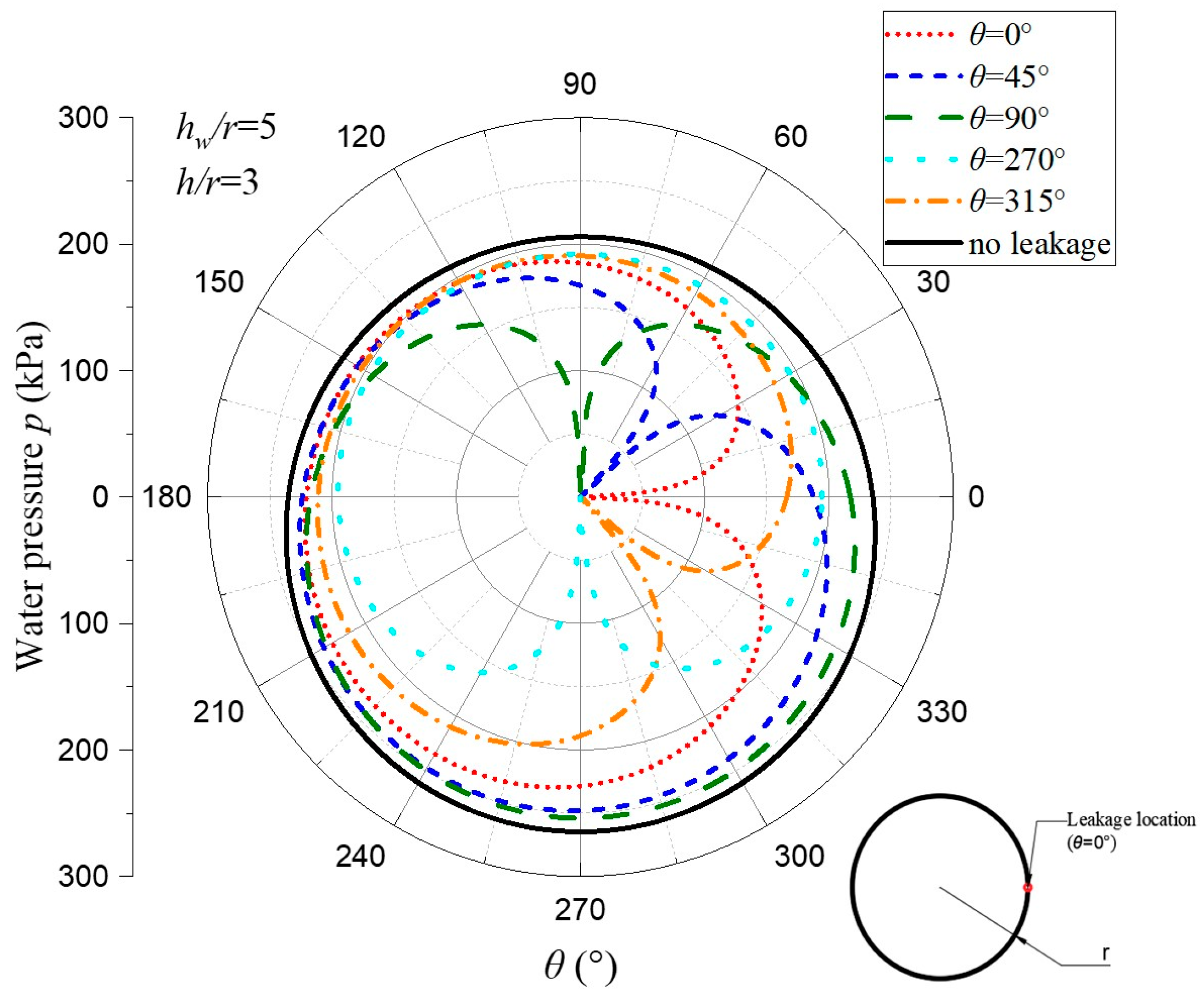
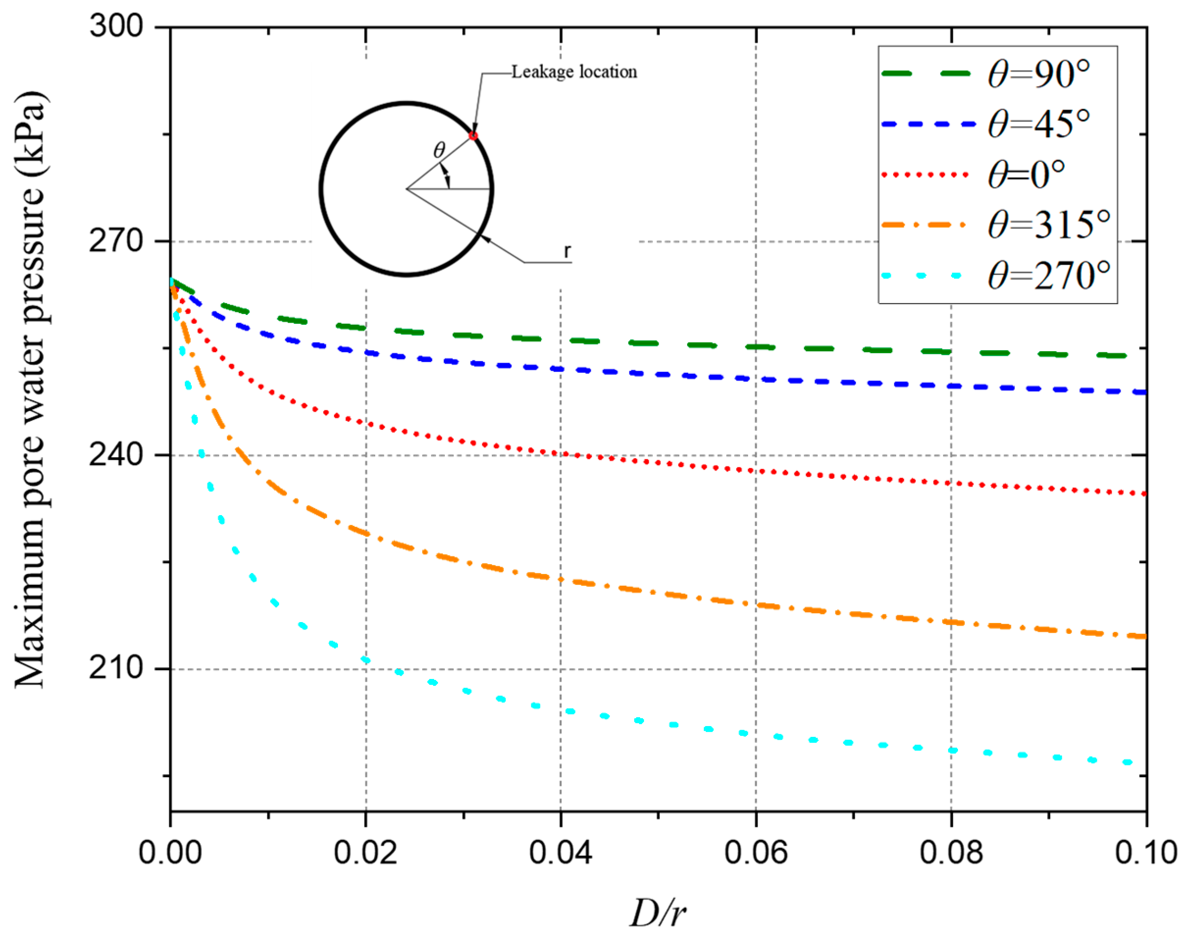
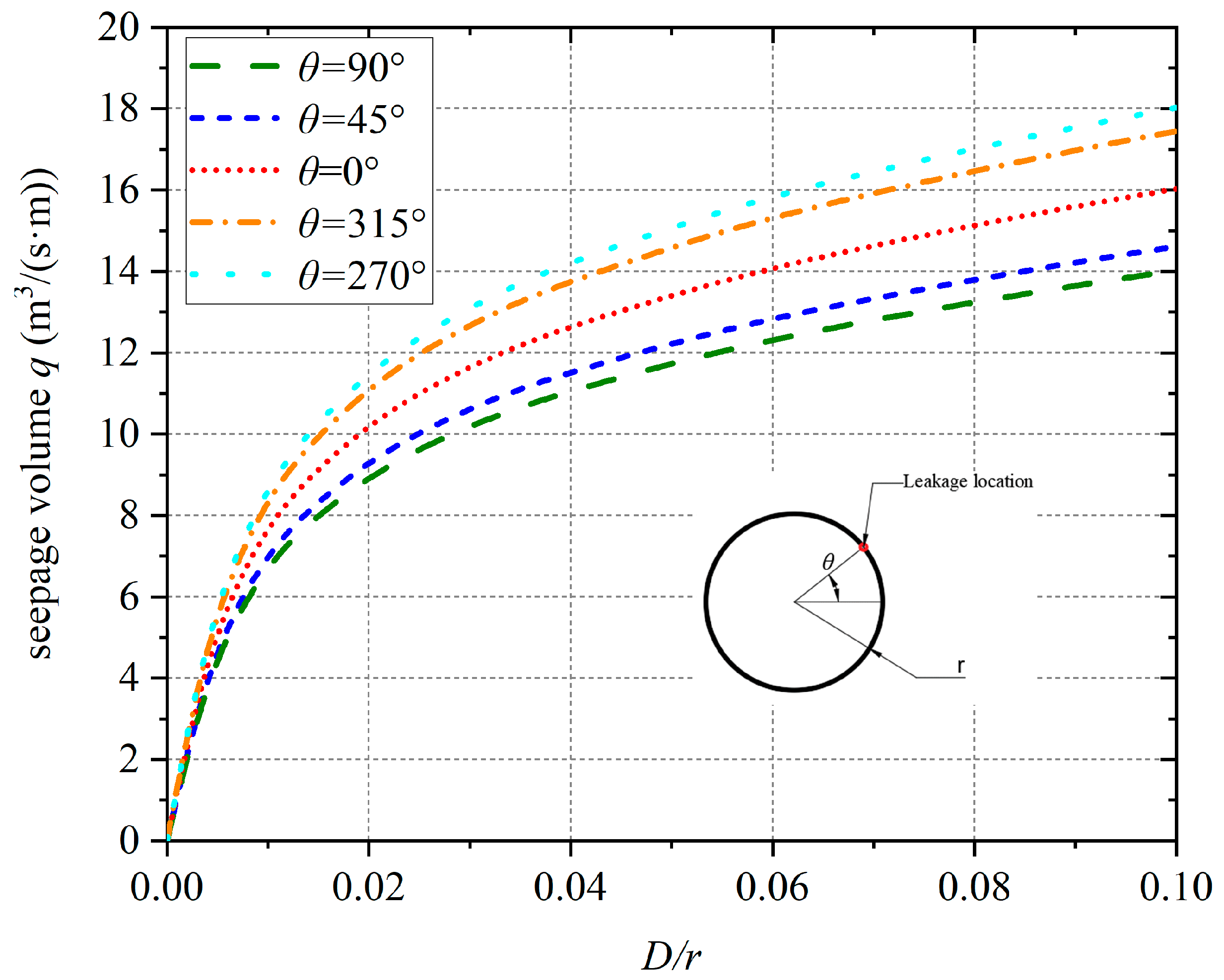
5.1. Leakage Location

Figure 8 shows the effect of the leakage location on the water pressure. The minimum water pressure occurs at the leakage locations as zero water pressure. Compared to the hydrostatic pressure without leakage, the water pressure within θ < 120° is significantly reduced, while the reduction is smaller for the lining away from the leakage location. This provides a reference for the design of drainage holes in tunnels in high-pressure water-rich areas to select an appropriate location of the hole for effectively reducing the water pressure outside the lining. In addition, it can be seen from Figure 8 that when θ = 270°, 315°, 0°, 45°, and 90°, the maximum pore water pressure on the tunnel lining is 197 kPa, 214 kPa, 234 kPa, 248 kPa, and 254 kPa, the location of the maximum pore water pressure on the tunnel lining is 147°, 214°, 238°, 256°, and 270°, and the angle difference from the leakage location is 123°, 101°, 122°, 149°, and 180°, respectively. Therefore, as the leakage location moves from the top of the tunnel to the bottom of the tunnel, the maximum pore water pressure on the tunnel lining gradually decreases. The location of the maximum pore water pressure also gradually moves closer to the leakage location, until the leakage location is close to the bottom of the tunnel, and the location of the maximum pore water pressure is slightly away from the leakage location.

Figure 9 shows the effect of the leakage location on the maximum water pressure over the tunnel lining. As the leakage moves from the top to the bottom of the tunnel, the maximum water pressure on the lining gradually decreases. The maximum water pressure on the lining when the leakage is at the bottom of the tunnel is only 0.77 times that of the leakage at the top of the tunnel. The most significant effect on reducing water pressure on the tunnel lining occurs when the leakage is at the bottom of the tunnel, which could provide a reference for the placement of tunnel drainage holes in high-pressure water-rich areas. In addition, it can be seen from Figure 9 that when the leakage is located in the lower half of the tunnel, the variation in the maximum pore water pressure is more obvious than when the leakage is located in the upper half of the tunnel. This phenomenon has been shown in other similar studies [4,30]. The reason for this phenomenon is that as the leakage location moves from the top of the tunnel to the bottom of the tunnel, in addition to the gradual increase in the seepage inflow into the tunnel that will lead to a decrease in the maximum pore water pressure of the tunnel lining, the reduction in the distance between the location of the maximum pore water pressure and the leakage site, and the increase in the effect of the leakage site on the reduction in the pore water pressure at the location of the maximum pore water pressure will also aggravate the decrease in the maximum pore water pressure of the tunnel lining. The conclusion that the distance between the maximum pore water pressure location and the leakage site decreases as the leakage location moves from the top of the tunnel to the bottom of the tunnel is shown in the analysis of Figure 8.

Figure 10 shows the effect of the leakage location on the seepage volume. As seen from the figure, the seepage volume minimizes and maximizes when the leakage is at the top/bottom of the tunnel. When the leakage is at the top of the tunnel, the seepage volume is only 0.78 times that of the leakage at the bottom of the tunnel. This is because, as the leakage location moves from the top to the bottom, the hydraulic head at the leakage location decreases while the hydraulic gradient increases. They jointly increase seepage flow.

5.2. Tunnel Depth

Figure 11 shows the effect of the tunnel burial depth on the water pressure in the tunnel lining. As the tunnel depth increases, the water pressure also increases. When h/r = 3, the water pressure within 120° of the localized water leakage location is less than 0.82 times the hydrostatic pressure; when h/r = 6, the water pressure within 120° of the localized water leakage location is less than 0.76 times the hydrostatic pressure; and when h/r = 9, the water pressure within 120° of the localized water leakage location is less than 0.74 times the hydrostatic pressure. It can be seen that the greater the depth of the tunnel burial is, the greater the effect of the water leakage on reducing the water pressure. Figure 12 shows the effect of the burial depth on the maximum water pressure over the tunnel lining. The figure shows that the maximum water pressure increases linearly with the increasing burial depth, regardless of the leakage location.

Figure 13 shows the effect of the tunnel depth on the seepage volume. As seen from the figure, regardless of leakage location, the seepage volume decreases and increases as the tunnel depth increases. This is because when h/r is small, the tunnel is close to the surface, and the surface water can easily flow through the soil layer above the tunnel. However, as the tunnel depth increases, it becomes difficult for the surface water to flow into the tunnel, decreasing the seepage volume at first. Then, as the tunnel depth increases further, the hydraulic head and gradient at the leakage location gradually decrease and increase, thus increasing the seepage volume. Therefore, the seepage volume will have a minimum value as the tunnel burial depth changes. It can also be seen in Figure 13 that as the location of the seepage moves from the top of the tunnel to the bottom of the tunnel, the burial depth at which the minimum value of seepage volume occurs increases.

5.3. Leakage Width

Figure 14 shows the influence of the leakage width on the water pressure. The water pressure on the tunnel lining decreases as the leakage width increases. This effect is more significant around the leakage location and smaller away from the leakage.

Figure 15 and Figure 16 show the effect of the leakage width on the maximum water pressure and the volume of the seepage flow. No matter where the leakage occurs, as the leakage width increases, the maximum water pressure on the tunnel lining decreases, and the seepage volume increases. It can be seen from Figure 16 that when the leakage position θ = 270° and D/r increases from 0 to 1/30, the maximum water pressure of the lining decreases by 58.7 kPa, and the seepage volume increases by 13.5 m³/(s·m). But when the leakage position θ = 270° and D/r increases from 1/30 to 1/10, the maximum water pressure of the lining only decreases by 9.1 kPa, and the seepage volume only increases by 4.5 m³/(s·m). It is apparent that when D/r is larger than 1/30, the reduction in maximum water pressure and the increase in seepage volume are significantly less than the ones when the leakage width is less than 1/30.

Therefore, as long as the leakage width is small (D/r less than 1/30), groundwater inflow can be effectively stopped, provided the leaking area is repaired promptly.

6. Concluding Remarks

This paper proposes an analytical solution for a seepage field when a local line leakage occurs in a tunnel based on the conformal transformation and the separated variable method, which overcomes the problem of current methods using the equivalent method or a method improving on the existing analytical solution for fully drained tunnels being unable to give an accurate analytical solution. In the solution process, the boundary conditions of the leakage site are accurately considered by the subregion method, and the principle of orthogonality of trigonometric functions is purposely used to construct a non-homogeneous system of equations for solving the unknowns in the analytical solution. Finally, it is validated against numerical simulation and experimental results and demonstrated by parametric analysis. This study suggests the following conclusions:

• The hydraulic head and water pressure results calculated by the proposed solution agree with the simulation results of the numerical software, which thus validate the analytical solution. The results of the seepage volume calculation were compared with the existing numerical solutions and the experimental results. It was found that the solution proposed in this paper was almost the same as the existing numerical solution, with a maximum error of 2.5%. It also agrees well with the experimental solution. Regarding the simulation and experimental results, the proposed solution outperforms other existing solutions by far in terms of accuracy.
• Compared with the numerical simulation, the total calculation time of the analytical solution is computationally more efficient, as shown by the fact that it only needs less than 1 s to carry out one case. And this analytical solution does avoid the tedious model, grid, and simulation process in the numerical software. As the solution yields comparable accuracy to numerical software, it is a reliable alternative when the computational efficiency is sensitive; for example, in parametric analysis.
• A parametric analysis of the effects of leak location, tunnel burial depth, and leakage width on the pore pressure distribution, maximum pore pressure, and seepage flow volume is enabled by virtue of the analytical solution. The analysis results suggest the influence of some factors, explanations of the phenomenon observed, and advice on applying this solution. These could be utilized in practice to improve the prediction of local line leakage and mitigate its adverse effects.

References

1. Zhou, Z.; Ding, H.H.; Miao, L.W.; Gong, C. Predictive model for the surface settlement caused by the excavation of twin tunnels. Tunn. Undergr. Space Technol. 2021, 114, 104014. [Google Scholar] [CrossRef]
2. Lei, M.F.; Zhu, B.B.; Gong, C.J.; Ding, W.; Liu, L. Sealing performance of a precast tunnel gasketed joint under high hydrostatic pressures: Site investigation and detailed numerical modeling. Tunn. Undergr. Space Technol. 2021, 115, 104082. [Google Scholar] [CrossRef]
3. Zhang, W.D.; Lei, L.; Zhou, P.P.; Li, D.W.; Mu, T.H. Analysis of Tunnel Leakage on Existing Railways and Treatment Technology. China Railw. 2022, 5, 125–129. [Google Scholar]
4. Liu, Y.; Zhang, D.M.; Huang, H.W. Influence of long-term partial drainage of shield tunnel on tunnel deformation and surface settlement. Rock Soil Mech. 2013, 34, 290–298. [Google Scholar]
5. Mair, R.J. Tunnelling and geotechnics: New horizons. Géotechnique 2008, 58, 695–736. [Google Scholar] [CrossRef]
6. Wongsaroj, J.; Soga, K.; Mair, R.J. Modelling of long-term ground response to tunnelling under St James’s Park, London. In Stiff Sedimentary Clays: Genesis and Engineering Behaviour: Géotechnique Symposium in Print 2007; Thomas Telford Ltd.: London, UK, 2011; pp. 253–268. [Google Scholar]
7. Yuan, Y.; Bai, Y.; Liu, J. Assessment service state of tunnel structure. Tunn. Undergr. Space Technol. 2012, 27, 72–85. [Google Scholar] [CrossRef]
8. Arjnoi, P.; Jeong, J.H.; Kim, C.Y.; Park, K.H. Effect of drainage conditions on porewater pressure distributions and lining stresses in drained tunnels. Tunn. Undergr. Space Technol. 2009, 24, 376–389. [Google Scholar] [CrossRef]
9. Yang, J.; Yin, Z.Y.; Laouafa, F.; Hicher, P.Y. Numerical analysis of internal erosion impact on underground structures: Application to tunnel leakage. Geomech. Energy Environ. 2022, 31, 100378. [Google Scholar] [CrossRef]
10. Wu, H.M.; Shen, S.L.; Chen, R.P.; Zhou, A. Three-dimensional numerical modelling on localised leakage in segmental lining of shield tunnels. Comput. Geotech. 2020, 122, 103549. [Google Scholar] [CrossRef]
11. Harr, M.E. Groundwater and Seepage; McGraw-Hill: New York, NY, USA, 1962. [Google Scholar]
12. Lei, S. An analytical solution for steady flow into a Ttonnel. Groundwater 1999, 37, 23–26. [Google Scholar] [CrossRef]
13. Kolymbas, D.; Wagner, P. Groundwater ingress to tunnels–the exact analytical solution. Tunn. Undergr. Space Technol. 2007, 22, 23–27. [Google Scholar] [CrossRef]
14. Meng, W.; He, C.; Zhou, Z.H.; Yan, Q.; Yang, W.; Guo, D.; Chen, Z. Influence of constant total hydraulic head on pore pressure and water inflow of grouted tunnel calculated by complex variable method. Tunn. Undergr. Space Technol. 2023, 136, 105071. [Google Scholar] [CrossRef]
15. Park, K.H.; Owatsiriwong, A.; Lee, J.G. Analytical solution for steady-state groundwater inflow into a drained circular tunnel in a semi-infinite aquifer: A revisit. Tunn. Undergr. Space Technol. 2008, 23, 206–209. [Google Scholar] [CrossRef]
16. El Tani, M. Circular tunnel in a semi-infinite aquifer. Tunn. Undergr. Space Technol. 2003, 18, 49–55. [Google Scholar] [CrossRef]
17. Huangfu, M.; Wang, M.S.; Tan, Z.S. Analytical solutions for steady seepage into an underwater circular tunnel. Tunn. Undergr. Space Technol. 2010, 25, 391–396. [Google Scholar] [CrossRef]
18. Zhang, D.M.; Huang, Z.K.; Yin, Z.Y.; Ran, L.Z.; Huang, H.W. Predicting the grouting effect on leakage-induced tunnels and ground response in saturated soils. Tunn. Undergr. Space Technol. 2017, 65, 76–90. [Google Scholar] [CrossRef]
19. Li, P.F.; Wang, F.; Long, Y.Y.; Zhao, X. Investigation of steady water inflow into a subsea grouted tunnel. Tunn. Undergr. Space Technol. 2018, 80, 92–102. [Google Scholar] [CrossRef]
20. Li, L.; Chen, H.H.; Li, J.P. A semi-analytical solution to steady-state groundwater inflow into a circular tunnel considering anisotropic permeability. Tunn. Undergr. Space Technol. 2021, 116, 104115. [Google Scholar] [CrossRef]
21. Li, Z.; He, C.; Chen, Z.; Yang, S.; Ding, J.; Pen, Y. Study of seepage field distribution and its influence on urban tunnels in water-rich regions. Bull. Eng. Geol. Environ. 2019, 78, 4035–4045. [Google Scholar] [CrossRef]
22. Zhu, C.W.; Wu, W.; Ying, H.W.; Gong, X.N.; Guo, P.P. Drainage-induced ground response in a twin-tunnel system through analytical prediction over the seepage field. Undergr. Space 2022, 7, 408–418. [Google Scholar] [CrossRef]
23. Guo, S.; Zhang, T.; Zhang, Y.; Zhu, D.Z. An approximate solution for two-dimensional groundwater infiltration in sewer systems. Water Sci. Technol. 2013, 67, 347–352. [Google Scholar] [CrossRef] [PubMed]
24. Tang, Y.; Chan, D.H.; Zhu, D.Z.; Guo, S. An analytical solution for steady seepage into a defective pipe. Water Sci. Technol. Water Supply 2018, 18, 926–935. [Google Scholar] [CrossRef]
25. Bear, J. Dynamics of Fluids in Porous Media; Elsevier Publishing Company: Amsterdam, The Netherlands, 1972. [Google Scholar]
26. Verruijt, A. A complex variable solution for a deforming circular tunnel in an elastic half-plane. Int. J. Numer. Anal. Methods Geomech. 1997, 21, 77–89. [Google Scholar] [CrossRef]
27. Gu, Q. Mathematical Methods for Physics; Science Press: Beijing, China, 2012. [Google Scholar]
28. Kirkham, D.; Powers, W.L. Advanced Soil Physics; Wiley: New York, NY, USA, 1972. [Google Scholar]
29. Li, D.K.; Yu, J.; Zheng, J.F.; Fan, Y. Analytical study of steady state seepage in a circular tunnel considering the outer boundary of the grouting ring as a non-constant head boundary. Tunn. Undergr. Space Technol. 2024, 144, 105510. [Google Scholar] [CrossRef]
30. Xu, G.W.; Lu, D.Y. Mechanical behavior of shield tunnel considering nonlinearity of flexural rigidity and leakage of joints. Chin. J. Geotech. Eng. 2016, 38, 1202–1211. [Google Scholar]
Figure 1. Diagram of the seepage analysis model for local line leakage in a tunnel.
Mathematics 13 00082 g001
Figure 2. Diagram of the conformal mapping process.
Mathematics 13 00082 g002
Figure 3. Diagram of superposition of boundary conditions by superposition method.
Mathematics 13 00082 g003
Figure 4. Comparison of the calculations of the seepage volume in the case of leakage from the top of the tunnel (The data comes from papers [23,24]).
Mathematics 13 00082 g004
Figure 5. Comparison of the seepage volume calculation results. (a) Varying leakage locations. (b) Varying leakage widths (The data comes from paper [24]).
Mathematics 13 00082 g005
Figure 6. Comparison of the hydraulic head calculation results.
Mathematics 13 00082 g006
Figure 7. Comparison of the results of the water pressure calculations on the tunnel lining.
Mathematics 13 00082 g007
Figure 8. Influence of the leakage location on the water pressure on the tunnel lining.
Mathematics 13 00082 g008
Figure 9. Influence of the leakage location on the maximum water pressure in the tunnel lining.
Mathematics 13 00082 g009
Figure 10. Influence of the leakage location on seepage volume.
Mathematics 13 00082 g010
Figure 11. Influence of the tunnel burial depth on the water pressure in the tunnel lining.
Mathematics 13 00082 g011
Figure 12. Influence of the tunnel burial depth on the maximum water pressure in the tunnel lining.
Mathematics 13 00082 g012
Figure 13. Influence of the tunnel burial depth on the seepage volume.
Mathematics 13 00082 g013
Figure 14. Influence of the leakage width on the water pressure on the tunnel lining.
Mathematics 13 00082 g014
Figure 15. Influence of the leakage width on the maximum water pressure over the tunnel lining.
Mathematics 13 00082 g015
Figure 16. Influence of the seepage width on the seepage volume.
Mathematics 13 00082 g016