New Insights on Keller–Osserman Conditions for Semilinear Systems

Abstract

In this article, we consider a semilinear elliptic system involving gradient terms of the form $\left\{\begin{array}{ccc}\Delta y\left(x\right)+{\lambda }_1\left|\nabla y\left(x\right)\right|=p\left(\left|x\right|\right)f\left(y\left(x\right),z\left(x\right)\right)\hfill & if\hfill & x\in \Omega ,\hfill \\ \Delta z\left(x\right)+{\lambda }_2\left|\nabla z\left(x\right)\right|=q\left(\left|x\right|\right)g\left(y\left(x\right)\right)\hfill & if\hfill & x\in \Omega ,\hfill \end{array}\right.$ where ${\lambda }_1$, ${\lambda }_2\in \left[0,\infty \right)$, $\Omega$ is either a ball of radius $R>0$ or the entire space ${\mathbb{R}}^N$. Based on certain standard assumptions regarding the potential functions p and q, we introduce new conditions on the nonlinearities f and g to investigate the existence of entire large solutions for the given system. The method employed is successive approximation. Additionally, for specific cases of p, q, f and g, we employ Python code to plot the graph of both the numerical solution and the exact solution.

1. Introduction

This paper analyzes a system of partial differential equations derived from a well-known partial differential equation that models a physical phenomenon, namely the time-independent Schrödinger equation. Specifically, we consider the semilinear elliptic system involving gradient terms of the form

$$\left\{\begin{array}{ccc}\Delta y\left(x\right)+{\lambda }_1\left|\nabla y\left(x\right)\right|=p\left(\left|x\right|\right)f\left(y\left(x\right),z\left(x\right)\right)\hfill & if\hfill & x\in \Omega ,\hfill \\ \Delta z\left(x\right)+{\lambda }_2\left|\nabla z\left(x\right)\right|=q\left(\left|x\right|\right)g\left(y\left(x\right)\right)\hfill & if\hfill & x\in \Omega ,\hfill \end{array}\right.$$

(1)

where ${\lambda }_1$, ${\lambda }_2\in \left[0,\infty \right)$, $\Omega =B_R\left(0\right)$ is either a ball of radius $R>0$ centered at the origin or the entire space ${\mathbb{R}}^N$, with certain assumptions on the functions p, q, f, g.

By their nature, the authors of scientific articles seek to address various problems in their field of study. Most of these can be discovered either through the study of a real-world phenomenon or through the analysis of various already published works. Our knowledge indicates that the system (1) is a derivative of the time-independent Schrödinger equation in quantum mechanics

$$(h^2/2m)\Delta w=(R-E)w$$

(2)

where $h=6.625·{10}^{-27}$ erg sec is the Planck constant, m is the mass of a particle moving under the action of a force field described by the potential $R(s,t,l),$ and $w(s,t,l)$ is the wave function. Here, E is the total energy of the particle.

However, even though this system (1) is derived from a partial differential equation of the type (2) that models a real phenomenon, it also appears in various fields of science and engineering. In particular, this system models the cost of a factory which plans its production as to minimize the production costs (see  [1,2]).

In Equation (2), the interest is to find the solution $w\left(r\right)$ such that

$$w\left(r\right)\to \infty \mathrm{as}r\to \infty ,r=\sqrt{s^2+t^2+l^2}$$

whence the motivation of our paper is to find analogous solutions for (1), specifically radially symmetric convex solutions that increases with r. That is, with notation

$$r=\left|x\right|=\sqrt{x_1^2+...+x_N^2},x=\left(x_1,...,x_N\right)\in \Omega \subseteq {\mathbb{R}}^N,$$

we need to prove the existence of a radially symmetric, convex and increasing solution for the system (1) of the type

$$y\left(r\right)\to \infty \mathrm{as}r\to \infty \mathrm{and}z\left(r\right)\to \infty \mathrm{as}r\to \infty .$$

(3)

This (3) is referred to as entire large radially symmetric solutions (large since it tends to infinity and entire as they are in ${\mathbb{R}}^N$). In this context, the system (1) can be expressed in radial form

$$\left\{\begin{array}{ccc}{\left(r^{N-1}{e}^{{\lambda }_{1}r}{y}^{\prime }\left(r\right)\right)}^{\prime }=r^{N-1}{e}^{{\lambda }_{1}r}p\left(r\right)f\left(y\left(r\right),z\left(r\right)\right)\hfill & if\hfill & r\in D,\hfill \\ {\left(r^{N-1}{e}^{{\lambda }_{2}r}{z}^{\prime }\left(r\right)\right)}^{\prime }=r^{N-1}{e}^{{\lambda }_{2}r}q\left(r\right)g\left(y\left(r\right)\right)\hfill & if\hfill & r\in D,\hfill \end{array}\right.$$

(4)

where $D=\left[0,R\right]$ if $\Omega =B_R$ and $D=\left[0,+\infty \right)$ if $\Omega ={\mathbb{R}}^N$.

In practical terms, the system (3)–(4) arises in the context of production planning problems involving multiple economic regimes.

In pure mathematics, the interest lies in introducing new conditions for the functions f and g that guarantee the existence of a solution to the system (4) with the boundary condition (3).

To accomplish our objective, we present our assumptions on p, q, f and g as follows:

(A1)   p, $q:D\to \left(0,\infty \right)$ are continuous functions on $\left[0,\infty \right)$;

(A2)   $f:\left[0,\infty \right)\times \left[0,\infty \right)\to \left[0,\infty \right)$ and $g:\left[0,\infty \right)\to \left[0,\infty \right)$ are continuous and nondecreasing in each variables such that for all $s,t>0$, we have $f\left(s,t\right)>0,$ $g\left(s\right)>0$;

(A3)   for all $s,r,l,t\ge 0$ we have $f\left(lt,sr\right)\le f\left(l,s\right)f\left(t,r\right)$;

(A4)   for $a\in \left(0,\infty \right)$ by setting $F:\left[a,\infty \right)\to \left[0,\infty \right)$ defined by

$$F\left(t\right)={\int }_a^t{\displaystyle \frac{1}{\sqrt{{\int }_0^{s}f\left(x,m_{1}g\left(x\right)\right)dx}}}ds\mathrm{for}t\ge a\mathrm{and}{m}_1\ge max\left\{1,{\displaystyle \frac{a}{g\left(a\right)}}\right\},$$

we assume

$$F\left(\infty \right)=\infty \mathrm{where}F\left(\infty \right):=\underset{t\to \infty }{lim}F\left(t\right).$$

Recently, two works seem to provide an answer to our problem. For instance, Wan–Shi [3] proposed conditions of the Keller–Osserman type

$${\int }_1^{\infty }{\displaystyle \frac{1}{\sqrt{{\int }_0^t(f\left(s,s\right)+g\left(s\right))ds}}}dt=\infty$$

(5)

and Wang–Zhang–Ahmad [4] of the Osgood type

$${\int }_1^{\infty }{\displaystyle \frac{1}{f\left(s,s\right)+g\left(s\right)}}ds=\infty$$

(6)

in order to fulfill the condition (3). Unfortunately, neither of these two results apply to the system

$$\left\{\begin{array}{ccc}{\left(r^{N-1}{y}^{\prime }\left(r\right)\right)}^{\prime }=r^{N-1}{y}^{\alpha }\left(r\right)z^{\beta }\left(r\right)\hfill & if\hfill & r\in D,\hfill \\ {\left(r^{N-1}{z}^{\prime }\left(r\right)\right)}^{\prime }=r^{N-1}{y}^{\gamma }\left(r\right)\hfill & if\hfill & r\in D,\hfill \end{array}\right. \alpha ,\beta ,\gamma \in \left[0,\infty \right)$$

(7)

for which Lair and Mohammed [5] proved that it has a positive entire large radial solution if and only if $\alpha$$\le 1$ and $\beta ·\gamma \le 1-\alpha$. Indeed, let us first note that conditions (5) and (6) are satisfied for

$$f\left(y,z\right)=y^{\alpha }{z}^{\beta }\mathrm{and}g\left(y\right)=y^{\gamma }$$

with positive parameters $\alpha ,\beta ,\gamma$ such that $\alpha +\beta +\gamma \le 1$. Our new assumption (A4) implies that $F\left(\infty \right)=\infty$ holds for $\alpha$, $\beta$, $\gamma$ with

$$\beta ·\gamma \le 1-\alpha ,$$

meaning that our new conditions encompass both sublinear and superlinear cases of the nonlinearities f and g considered by [5].

By fixing the conditions on p, $q,$ the assumptions (5), (6) and (A4) have a long history and have garnered significant interest from many researchers (see [3,5,6,7,8] and references therein).

In the paper by Padhi and Dix [8], the authors investigate the existence and asymptotic behavior of positive radial solutions to a system of nonlinear elliptic equations under similar conditions to those on functions f and g of the form (6). This research enhances the broader understanding of nonlinear elliptic systems and their applications. The study is inspired by previous works of [6,7] on similar systems and aims to present new findings in this field.

The paper by Wan and Shi [3] presents conditions that are significantly less restrictive than those in previous studies. This research advances the mathematical understanding of q-k-Hessian problems and introduces new solutions under conditions of the form (5). More recently, Wang, Zhang and Ahmad [4] achieved similar results under conditions of the form (6) for a k-Hessian system with gradient term.

This paper [9], authored by Andrey B. Muravnik, delves into the Keller–Osserman phenomena for Kardar–Parisi–Zhang (KPZ) type inequalities. The study extends classical results and provides new insights into the behavior of solutions in mathematical physics, particularly in the context of blow-up phenomena and the absence of global solutions.

A more comprehensive discussion on conditions of the form (5)–(6) is available in the recent works of [3,4]. Therefore, we will omit some additional details to focus on proving our results.

Theorem 1.

Assume $D=\left[0,R\right]$ and $N\ge 2$. If conditions (A1), (A2), (A3) and (A4) are satisfied, then (4) has a nonnegative solution in $C^2\left(D\right)\times C^2\left(D\right)$ such that $y\left(0\right)=z\left(0\right)=a$.

To formulate the next result, we denote by

$$\begin{array}{ccc}\hfill P\left(r\right)& =& {\int }_0^r{t}^{1-N}{e}^{-{\lambda }_{1}t}{\int }_0^t{s}^{N-1}{e}^{{\lambda }_{1}s}p\left(s\right)dsdt,\hfill \\ \hfill Q\left(r\right)& =& {\int }_0^r{t}^{1-N}{e}^{-{\lambda }_{2}t}{\int }_0^t{s}^{N-1}{e}^{{\lambda }_{2}s}q\left(s\right)dsdt\hfill \\ \hfill P_{\infty }& =& \underset{r\to \infty }{lim}{\int }_0^r{t}^{1-N}{e}^{-{\lambda }_{1}t}{\int }_0^t{s}^{N-1}{e}^{{\lambda }_{1}s}p\left(s\right)f\left(a,a+g\left(a\right)Q\left(s\right)\right)dsdt\hfill \\ \hfill Q_{\infty }& =& \underset{r\to \infty }{lim}{\int }_0^r{t}^{1-N}{e}^{-{\lambda }_{2}t}{\int }_0^t{s}^{N-1}{e}^{{\lambda }_{2}s}q\left(s\right)g\left(a+f\left(a,a\right)P\left(s\right)\right)dsdt\hfill \end{array}$$

and then our second result is:

Theorem 2.

Assume$D=\left[0,+\infty \right)$ and $N\ge 3$. If conditions (A1)–(A4) and $P_{\infty }=Q_{\infty }=\infty$ are satisfied, then (4) has a nonnegative, convex, entire large solution in $C^2\left[0,\infty \right)\times C^2\left[0,\infty \right)$ such that $y\left(0\right)=z\left(0\right)=a$.

Our strategy is to construct the solution as the limit of a monotonically increasing sequence within $D=\left[0,R\right]$ with $R>0$ arbitrary. By  appealing to the Arzela–Ascoli theorem, which states that the sequence is both bounded and equicontinuous on the $\left[0,R\right]$, we ensure that it contains a subsequence that converges to the solution in the entire space $\left[0,\infty \right)$. With this observation, we can prove both of our results together.

2. Proof of Theorems 1 and 2

Let us highlight that our goal is to find the solutions $y\left(r\right)$ and $z\left(r\right)$ that increase with r. To achieve this, we will consider the radial form

$$\left\{\begin{array}{ccc}{y}^{″}\left(r\right)+{\displaystyle \frac{N-1}{r}}{y}^{\prime }\left(r\right)+{\lambda }_1{y}^{\prime }\left(r\right)=p\left(r\right)f\left(y\left(r\right),z\left(r\right)\right)\hfill & if\hfill & r\in \left(0,R\right],\hfill \\ z^{″}\left(r\right)+{\displaystyle \frac{N-1}{r}}{z}^{\prime }\left(r\right)+{\lambda }_2{z}^{\prime }\left(r\right)=q\left(r\right)g\left(y\left(r\right)\right)\hfill & if\hfill & r\in \left(0,R\right],\hfill \\ y\left(0\right)=z\left(0\right)=a,\hfill & \hfill & \\ y^{\prime }\left(0\right)=z^{\prime }\left(0\right)=0,\hfill & \hfill \end{array}\right.$$

(8)

instead of the classical form (4)/(1). We will start by proving the existence of a radial convex, increasing solution $\left(y\left(r\right),z\left(r\right)\right)$. The system (8) can be written in the integral form

$$\left\{\begin{array}{ccc}y\left(r\right)=a+{\int }_0^r{t}^{1-N}{e}^{-{\lambda }_{1}t}{\int }_0^t{s}^{N-1}{e}^{{\lambda }_{1}s}p\left(s\right)f\left(y\left(s\right),z\left(s\right)\right)dsdt\hfill & if\hfill & r\in D,\hfill \\ z\left(r\right)=a+{\int }_0^r{t}^{1-N}{e}^{-{\lambda }_{2}t}{\int }_0^t{s}^{N-1}{e}^{{\lambda }_{2}s}q\left(s\right)g\left(y\left(s\right)\right)dsdt\hfill & if\hfill & r\in D.\hfill \end{array}\right.$$

(9)

Next, we define the sequences ${\left\{y_n\right\}}_{n\in \mathbb{N}}$ and ${\left\{z_n\right\}}_{n\in \mathbb{N}}$ on $\left[0,\infty \right)$ as below

$$\left\{\begin{array}{ccc}{y}_0\left(r\right)=y\left(0\right)=z_0\left(r\right)=z\left(0\right)=a\hfill & if\hfill & r\in D\hfill \\ y_n\left(r\right)=a+{\int }_0^r{t}^{1-N}{e}^{-{\lambda }_{1}t}{\int }_0^t{s}^{N-1}{e}^{{\lambda }_{1}s}p\left(s\right)f\left(y_{n-1}\left(s\right),z_{n-1}\left(s\right)\right)dsdt\hfill & if\hfill & r\in \left(0,R\right],\hfill \\ z_n\left(r\right)=a+{\int }_0^r{t}^{1-N}{e}^{-{\lambda }_{2}t}{\int }_0^t{s}^{N-1}{e}^{{\lambda }_{2}s}q\left(s\right)g\left(y_{n-1}\left(s\right)\right)dsdt\hfill & if\hfill & r\in \left(0,R\right].\hfill \end{array}\right.$$

(10)

A straightforward calculation reveals that ${\left\{y_n\right\}}_{n\in \mathbb{N}}$ and ${\left\{z_n\right\}}_{n\in \mathbb{N}}$ are nondecreasing on $\left[0,\infty \right)$; see, for example, [8]. For

$$m_1\ge max\left\{1,{\displaystyle \frac{a}{g\left(a\right)}}\right\}\mathrm{and}{m}_2\ge max\left\{1,{\displaystyle \frac{a}{f\left(a,a\right)}}\right\}$$

we have

$$\begin{array}{ccc}\hfill y_n\left(r\right)& =& a+{\int }_0^r{t}^{1-N}{e}^{-{\lambda }_{1}t}{\int }_0^t{s}^{N-1}{e}^{{\lambda }_{1}s}p\left(s\right)f\left(y_{n-1}\left(s\right),z_{n-1}\left(s\right)\right)dsdt\hfill \\ & \le & a+{\int }_0^r{t}^{1-N}{e}^{-{\lambda }_{1}t}{\int }_0^t{s}^{N-1}{e}^{{\lambda }_{1}s}p\left(s\right)f\left(y_n\left(s\right),z_n\left(s\right)\right)dsdt\hfill \\ & \le & a+f\left(y_n\left(r\right),z_n\left(r\right)\right){\int }_0^r{t}^{1-N}{e}^{-{\lambda }_{1}t}{\int }_0^t{s}^{N-1}{e}^{{\lambda }_{1}s}p\left(s\right)dsdt\hfill \\ & \le & f\left(y_n\left(r\right),z_n\left(r\right)\right)\left({\displaystyle \frac{a}{f\left(a,a\right)}}+P\left(r\right)\right)\hfill \\ & \le & m_{2}f\left(y_n\left(r\right),z_n\left(r\right)\right)\left(1+P\left(r\right)\right)\hfill \end{array}$$

and

$$z_n\left(r\right)\le m_{1}g\left(y_n\left(r\right)\right)\left(1+Q\left(r\right)\right).$$

Observe that, through direct calculation, we find that

$$\underset{r\to 0}{lim}{y}^{\prime }\left(r\right)y^{″}\left(r\right)=0.$$

Next, our aim is to prove that the sequences

$${\left\{y_n\right\}}_{n\in \mathbb{N}}\mathrm{and}{\left\{z_n\right\}}_{n\in \mathbb{N}}\mathrm{on}\left[0,R\right]$$

are bounded for arbitrary $R>0$. By setting

$$M_p=max\left\{p\left(s\right)\left|0\le r\le R\right.\right\}$$

we obtain

$$\begin{array}{ccc}\hfill 2y_n^{\prime }\left(r\right)y_n^{″}\left(r\right)& \le & 2\left(y_n^{″}\left(r\right)+{\displaystyle \frac{N-1}{r}}{y}_n^{\prime }\left(r\right)\right)y_n^{\prime }\left(r\right)\hfill \\ & =& 2\left[p\left(r\right)f\left(y_n\left(r\right),z_n\left(r\right)\right)-{\lambda }_1{y}_n^{\prime }\left(r\right)\right]y_n^{\prime }\left(r\right)\hfill \\ & \le & 2M_{p}f\left(y_n\left(r\right),z_n\left(r\right)\right)y_n^{\prime }\left(r\right)\hfill \\ & \le & 2M_{p}f\left(y_n\left(r\right),m_{1}g\left(y_n\left(r\right)\right)\left(1+Q\left(r\right)\right)\right)y_n^{\prime }\left(r\right)\hfill \\ & \le & 2M_{p}f\left(1,1+Q\left(r\right)\right)f\left(y_n\left(r\right),m_{1}g\left(y_n\left(r\right)\right)\right)y_n^{\prime }\left(r\right).\hfill \end{array}$$

This can be expressed in an equivalent form

$$\begin{array}{ccc}{\left[{\left(y_n^{\prime }\left(r\right)\right)}^2\right]}^{\prime }\le 2M_{p}f\left(1,1+Q\left(r\right)\right)f\left(y_n\left(r\right),m_{1}g\left(y_n\left(r\right)\right)\right)y_n^{\prime }\left(r\right)& if& r\in \left[0,R\right].\end{array}$$

Integrating this inequality over $\left[0,r\right]$, we obtain

$$\begin{array}{ccc}{y}_n^{\prime }\left(r\right)\le \sqrt{2M_{p}f\left(1,1+Q\left(r\right)\right)}\sqrt{{\int }_a^{y_n\left(r\right)}f\left(z,m_{1}g\left(z\right)\right)dz}& if& r\in \left[0,R\right],\end{array}$$

or, equivalently

$$\begin{array}{ccc}{\displaystyle \frac{y_n^{\prime }\left(r\right)}{\sqrt{{\int }_a^{y_n\left(r\right)}f\left(z,m_{1}g\left(z\right)\right)dz}}}\le \sqrt{2M_{p}f\left(1,1+Q\left(r\right)\right)}& if& r\in \left[0,R\right],\end{array}$$

By integrating once more from 0 to $R\in \left[0,\infty \right)$, we obtain

$$\begin{array}{c}{\int }_a^{y_n\left(R\right)}{\displaystyle \frac{1}{\sqrt{{\int }_a^{t}f\left(z,m_{1}g\left(z\right)\right)dz}}}dt\le R\sqrt{2M_{p}f\left(1,1+Q\left(R\right)\right)}.\end{array}$$

Consequently,

$$\begin{array}{ccc}F\left(y_n\left(R\right)\right)\le R\sqrt{2M_{p}f\left(1,1+Q\left(R\right)\right)}& if& R\in \left[0,\infty \right).\end{array}$$

It is necessary to establish certain properties for F. Firstly, the  function F is bijective on their domains, ensuring the existence of their inverses $F^{-1}$ of F. Secondly, since

$$F^{\prime }\left(t\right)\ge 0\mathrm{for}\mathrm{all}t\ge a$$

this implies that $F^{-1}$ is a monotonically increasing function on their domain. The  last observation is that

$$F\left(a\right)=0⟹a=F^{-1}\left(0\right)\mathrm{and}F\left(\infty \right)=\infty ⟹\infty =F^{-1}\left(\infty \right).$$

In summary, due to the fact that

$$r\to y_n\left(r\right)$$

is increasing for all $r\in D$, it follows that

$$y_n\left(r\right)\le y_n\left(R\right),\mathrm{for}\mathrm{all}r\in \left[0,R\right].$$

On the other hand, by coupling this inequality with

$$\begin{array}{ccc}{y}_n\left(R\right)\le F^{-1}\left(R\sqrt{2M_{p}f\left(1,1+Q\left(R\right)\right)}\right)& if& R\in D,\end{array}$$

and

$$z_n\left(r\right)\le m_{1}g\left(y_n\left(r\right)\right)\left(1+Q\left(r\right)\right)\mathrm{for}\mathrm{all}r\in D$$

we obtain

$$y_n\left(r\right)\le F^{-1}\left(R\sqrt{2M_{p}f\left(1,1+Q\left(R\right)\right)}\right)\mathrm{on}\left[0,R\right]$$

and

$$z_n\left(r\right)\le m_{1}g\left(F^{-1}\left(R\sqrt{2M_{p}f\left(1,1+Q\left(R\right)\right)}\right)\right)\left(1+Q\left(R\right)\right)\mathrm{on}\left[0,R\right].$$

with arbitrary R.

Given that the sequences ${\left\{y_n\right\}}_{n\in \mathbb{N}}$ and ${\left\{z_n\right\}}_{n\in \mathbb{N}}$ are bounded and monotonically increasing on $\left[0,R\right]$, the limit function serves as the solution to the problem (4). Thus, the proof of Theorem 1 is concluded.

Finally, it remains to prove Theorem 2. Given that

$$\left\{\begin{array}{ccc}{y}_n^{\prime }\left(r\right)=r^{1-N}{e}^{-{\lambda }_{1}r}{\int }_0^r{s}^{N-1}{e}^{{\lambda }_{1}s}p\left(s\right)f\left(y_{n-1}\left(s\right),z_{n-1}\left(s\right)\right)ds\hfill & if\hfill & r\ge 0,\hfill \\ z_n^{\prime }\left(r\right)=r^{1-N}{e}^{-{\lambda }_{2}r}{\int }_0^r{s}^{N-1}{e}^{{\lambda }_{2}s}q\left(s\right)g\left(y_{n-1}\left(s\right)\right)ds\hfill & if\hfill & r\ge 0,\hfill \end{array}\right.$$

we establish the boundedness of ${\left\{y_n^{\prime }\right\}}_{n\in \mathbb{N}}$ and ${\left\{z_n^{\prime }\right\}}_{n\in \mathbb{N}}$ on $\left[0,R\right]$ for arbitrary $R\in \left[0,\infty \right)$, in the same manner as previously proved. This confirms that the sequences ${\left\{y_n\right\}}_{n\in \mathbb{N}}$ and ${\left\{z_n\right\}}_{n\in \mathbb{N}}$ are both bounded and equicontinuous on $\left[0,R\right]$ for arbitrary $R>0$. Hence, by the Arzela–Ascoli theorem, the subsequences of ${\left\{\left(y_n,z_n\right)\right\}}_{n\in \mathbb{N}}$ converges uniformly to $\left(y,z\right)$ on $\left[0,R\right]$ for arbitrary $R>0$. The monotonicity of the sequence ${\left\{\left(y_n,z_n\right)\right\}}_{n\in \mathbb{N}}$ ensures that the convergence to $\left(y,z\right)$ remains valid on $\left[0,\infty \right)$. Taking the limit in (10), we obtain that $\left(y\left(r\right),z\left(r\right)\right)$ satisfies (9), thus proving it is the solution of (8). The fact that y and z are convex and that

$$\left(y,z\right)\in C^2\left(\left[0,\infty \right)\right)\times C^2\left(\left[0,\infty \right)\right)$$

yields by a standard calculation. Thus, (4) has a nonnegative, convex and nontrivial solution in $C^2\left[0,\infty \right)\times C^2\left[0,\infty \right)$, denoted by $\left(y,z\right)$. To determine the limit of the solution, we first note that

$$a+f\left(a,a\right)P\left(r\right)\le y\left(r\right)\mathrm{for}\mathrm{all}r\in \left[0,\infty \right),$$

(11)

and

$$a+g\left(a\right)Q\left(r\right)\le z\left(r\right),\mathrm{for}\mathrm{all}r\in \left[0,\infty \right).$$

(12)

The next step is to observe that by using (11) and (12) in (9), we obtain

$$\begin{array}{ccc}\hfill y\left(r\right)& =& a+{\int }_0^r{t}^{1-N}{e}^{-{\lambda }_{1}t}{\int }_0^t{s}^{N-1}{e}^{{\lambda }_{1}s}p\left(s\right)f\left(y\left(s\right),z\left(s\right)\right)dsdt\hfill \\ & \ge & a+{\int }_0^r{t}^{1-N}{e}^{-{\lambda }_{1}t}{\int }_0^t{s}^{N-1}{e}^{{\lambda }_{1}s}p\left(s\right)f\left(a,a+g\left(a\right)Q\left(s\right)\right)dsdt\hfill \end{array}$$

(13)

and

$$\begin{array}{ccc}\hfill z\left(r\right)& =& a+{\int }_0^r{t}^{1-N}{e}^{-{\lambda }_{2}t}{\int }_0^t{s}^{N-1}{e}^{{\lambda }_{2}s}q\left(s\right)g\left(y\left(s\right)\right)dsdt\hfill \\ & \ge & a+{\int }_0^r{t}^{1-N}{e}^{-{\lambda }_{2}t}{\int }_0^t{s}^{N-1}{e}^{{\lambda }_{2}s}q\left(s\right)g\left(a+f\left(a,a\right)P\left(s\right)\right)dsdt\hfill \end{array}$$

(14)

by passing to the limit as $r\to \infty$ in (13)–(14), we clearly have

$$y\left(r\right)\to P_{\infty }\mathrm{as}r\to \infty$$

and

$$z\left(r\right)\to Q_{\infty }\mathrm{as}r\to \infty .$$

At this point, it is evident that the solution is entirely large, thus proving Theorem 2.

3. A Python Code to Plot the Solution

In this section, we provide the Python code to plot the numerical solution for the system (4), for the case

$${\lambda }_1={\lambda }_2=1,p\left(r\right)={\displaystyle \frac{4r^3+20r^2}{\sqrt{r^2+1}}},q\left(r\right)={\displaystyle \frac{2r+6}{r^4+1}},f\left(y,z\right)=\sqrt{z},g\left(y\right)=y,N=3$$

(15)

and the exact solution

$$y_{exact}\left(r\right)=r^4+1\mathrm{and}{z}_{exact}\left(r\right)=r^2+1$$

under the same settings.

This is possible with the assistance of [10]:

import numpy as np

import math

import matplotlib.pyplot as~plt

# Define the system of differential equations

def system(r, Y):

    y, dy, z, dz = Y

    d2y = ((4 * r**3 + 20 * r**2) / math.sqrt(r**2 + 1)) * math.sqrt(z)

    - (2 / r) * dy - dy

    d2z = ((2 * r + 6) / (r**4 + 1)) * y - (2 / r) * dz - dz

    return [dy, d2y, dz, d2z]

# Initial conditions

Y0 = [1, 0, 1, 0]

# Successive approximation method

def successive_approximation(system, r_span, Y0, tol=0.000001, max_iter=1):

    r_eval = np.linspace(r_span[0], r_span[1], 100)

    Y = np.zeros((4, len(r_eval)))

    Y[:, 0] = Y0

    for i in range(1, len(r_eval)):

        r = r_eval[i]

        Y_prev = Y[:, i-1]

        for _ in range(max_iter):

            Y_new = Y_prev + np.array(system(r, Y_prev)) * (r_eval[i]

            - r_eval[i-1])

            if np.linalg.norm(Y_new - Y_prev) < tol:

                break

            Y_prev = Y_new

        Y[:, i] = Y_new

    return r_eval, Y

# Solve the system

r_span = (0.1, 1.4)

r_eval, sol = successive_approximation(system, r_span, Y0)

# Define the range of x

t = np.linspace(0.1, 1.4, 100)

# Exact solutions

y_exact = t**4 + 1

z_exact = t**2 + 1

# Plot the numerical solution

plt.figure(figsize=(10, 5))

plt.subplot(1, 2, 1)

plt.plot(r_eval, sol[0], label=’y(r)’)

plt.plot(r_eval, sol[2], label=’z(r)’)

plt.xlabel(’r’)

plt.ylabel(’Numerical Solution’)

plt.legend()

plt.title(’Numerical Solution of the System’)

# Plot the exact solution

plt.subplot(1, 2, 2)

plt.plot(t, y_exact, label=’y_exact(t)’, linestyle=’dashed’)

plt.plot(t, z_exact, label=’z_exact(t)’, linestyle=’dashed’)

plt.xlabel(’t’)

plt.ylabel(’Exact Solution’)

plt.legend()

plt.title(’Exact Solution of the System’)

plt.tight_layout()

plt.show()

Under the conditions specified in (15), running the above code will yield the following result:

Number of Iterations (max_iter)	1
Tolerance (tol)	$0.000001$
Initial Values (Y0)	$\left\{\begin{array}{c}y\left(0\right)=1,y^{\prime }\left(0\right)=0\\ z\left(0\right)=1,z^{\prime }\left(0\right)=0\end{array}\right.$
Range of r and t	$\left[0.1,1.4\right]$
The evenly spaced values within the range of r and t	100

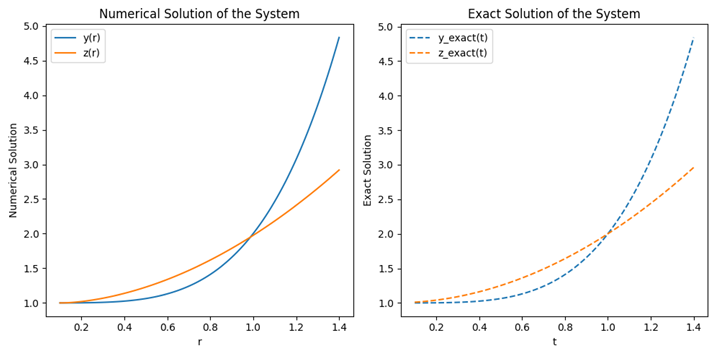
Clearly, increasing the number of iterations enhances the likelihood of the method converging to an accurate solution. Interestingly, by visually comparing the numerical and exact solutions on the plot, we observe that the numerical solution rapidly converges to the exact solution.

4. Conclusions

We have derived new conditions on the nonlinearities f and g to investigate the existence of positive radial solutions for a system involving the Laplacian operator. The result is validated through an example using Python code. This study encompasses both sublinear and superlinear cases as considered by [5] in a specific context.

References

- Cadenillas, A.; Ferrari, G.; Schuhmann, P. Optimal productionmanagement when there is regime switching and production constraints. Ann. Oper. Res. 2024, 1–33. [Google Scholar] [CrossRef]
- Covei, D.-P. Exact Solution for the Production Planning Problem with Several Regimes Switching over an Infinite Horizon Time. Mathematics 2023, 11, 4307. [Google Scholar] [CrossRef]
- Wan, H.; Shi, Y. Sharp conditions for the existence of infinitely many positive solutions to q-k-Hessian equation and systems. Electron. Res. Arch. 2024, 32, 5090–5108. [Google Scholar] [CrossRef]
- Wang, G.; Zhang, Z.; Ahmad, B. On the existence of radial solutions to a nonlinear k-Hessian system with gradient term. Nonlinear Anal. Real World Appl. 2025, 82, 104255. [Google Scholar] [CrossRef]
- Lair, A.V.; Mohammed, A. Large solutions to semi-linear elliptic systems with variable exponents. J. Math. Anal. Appl. 2014, 420, 1478–1499. [Google Scholar] [CrossRef]
- Covei, D.-P. A remark on the existence of entire large positive radial solutions to nonlinear differential equations and systems. J. Math. Anal. Appl. 2023, 519, 126824. [Google Scholar] [CrossRef]
- Covei, D.-P. A system of two elliptic equations with nonlinear convection and coupled reaction terms. Quaest. Math. 2024, 47, 437–450. [Google Scholar] [CrossRef]
- Padhi, S.; Dix, J.G. Existence of positive global radial solutions to nonlinear elliptic systems. Electron. J. Differ. Equ. 2023, 02, 231–238. [Google Scholar] [CrossRef]
- Muravnik, A.B. Keller–Osserman Phenomena for Kardar–Parisi–Zhang-Type Inequalities. Mathematics 2023, 11, 3787. [Google Scholar] [CrossRef]
- Microsoft Copilot in Edge. 2024. Available online: https://www.microsoft.com/en-us/edge/features/copilot?form=MA13FJ (accessed on 26 December 2024).
Disclaimer/Publisher’s Note: The statements, opinions and data contained in all publications are solely those of the individual author(s) and contributor(s) and not of MDPI and/or the editor(s). MDPI and/or the editor(s) disclaim responsibility for any injury to people or property resulting from any ideas, methods, instructions or products referred to in the content. |
© 2024 by the author. Licensee MDPI, Basel, Switzerland. This article is an open access article distributed under the terms and conditions of the Creative Commons Attribution (CC BY) license (https://creativecommons.org/licenses/by/4.0/).