Qualitatively New Approach to Business Valuation and Company Value

Abstract

The objective of this work is to develop a qualitative new approach to assessing business and company value. For this purpose, two of the three income approach methods, CAPM and WACC, are modified. When modifying CAPM, a new model, CAPM 2.0, was created, within which business and financial risks were simultaneously taken into account. Moreover, for the first time, this was performed correctly and the inaccuracy, incorrectness and inconsistency of the popular Hamada model were shown. The developed approach corrects some of the shortcomings of the income approach. The new methodology significantly improves the accuracy of the assessment. The closeness of the results of the new methodology to the actual market value of Amazon company (AMZN) shows the importance and validity of this methodology, which should be used to evaluate the business and the value of the company.

1. Introduction

The value of any asset (stocks, bonds, companies, etc.) is equal to the present value of all income generated by that asset. Thus, to find the value of a company, it is necessary to find the current value of all the income received by the company from its inception to the current moment, that is, in the retrospective period. And to evaluate a business, it is necessary to find the current value of all future income received by the enterprise in the representative and terminate periods.

Business valuation goals could be as follows: purchase and sale of company shares and bonds on the stock market; making an informed investment decision; purchase and sale of a company; company restructuring; liquidation, merger, acquisition, spin-off of an independent company; determining the company’s creditworthiness and the value of collateral for lending; insurance; taxation; making informed management decisions; etc.

A company’s market capitalization is very important to investors: it shows the company’s position in the market and determines how much investors are willing to pay for its shares. The greatest interest is in blue chip companies (with a capitalization above USD 10 billion), which are leaders in their industry and are less susceptible to market volatility.

In this paper, the new approach to business valuation and company value has been developed. As is well known, there are three main methods in business valuation: cost, comparative and income, with the latter being the most adequate and accurate. There are three approaches to the income method: CAPM, APT and WACC. This article presents modifications of two of these three methods: CAPM and WACC. When modifying CAPM, a new model, CAPM 2.0, was created, within which business and financial risks were simultaneously taken into account. Moreover, for the first time, this was performed correctly and the inaccuracy, incorrectness and inconsistency of the popular Hamada model were shown. When modifying the WACC approach (or the discounted income method), the following shortcomings of the income approach were corrected: inability of appraisers to correctly estimate the discount rate, the value of which is the main value in the income method of business valuation; the absence (before the advent of the BFO theory) of a correct method for estimating the discount rate; incorrect accounting of the influence of the retrospective period. The CAPM and CAPM 2.0 models have been incorporated into two major theories of capital structure—the Brusov–Filatova–Orekhova (BFO) theory and the Modigliani–Miller (MM) theory: this allows an account of both business and financial risks. CAPM takes into account systematic (business) risk, while capital structure theories take into account the financial risk of a specific company, associated with debt financing.

1.1. Disadvantage of Existing Valuation Methods (Income Approach)

The most important drawback of existing assessment methods is their inability to estimate the main assessment parameter—the discount rate, the value of which is critical in the assessment. The role of the correct determination of the discount rate in preventing abuse in business valuation, in investments, in determining the fair value of dividend income of shareholders is crucial. In business valuation, unscrupulous appraisers manipulate the value of the discount rate for the raider capture of enterprises. In investments, an incorrect assessment of the discount rate leads to an incorrect assessment of the effectiveness of an investment project, does not allow ranking investment projects in order to select the most effective projects in conditions of limited investment resources (companies, municipal and state). This can lead to misappropriation of public funds, including funds from national projects. The rights of shareholders to receive adequate profits can be violated when the company’s management conducts an incorrect and ineffective dividend policy, due to the inability of the management to determine the correct amount of dividends (the economically justified amount of which is the equity cost), or with the deliberate violation of shareholders’ rights in this area.

Currently, there is only one theory that allows us to correctly estimate the discount rate—the BFO theory. Within the framework of the BFO theory, it is possible to study the dependence of WACC on the age of the company. This makes it possible to link a retrospective analysis of the company financial state with a representative one.

One more disadvantage of DCF (discounted cash flow) is its reliance on estimations of future cash flows, which could prove inaccurate. The BFO theory allows us to improve this shortcoming in two directions, using data on financial flows over the past few years. By determining the rate of income growth, we can (1) improve the forecasting of financial flows in representative and tentative periods; (2) use a modification of the BFO theory for the case of variable income, which we recently obtained, to correctly determine the discount rate WACC, which in this case depends on the rate of income growth.

1.2. Literature Review

As it was mentioned above, there are three main methods for estimating the value of assets. The first method is the well-known CAPM (capital asset pricing model), which uses the risk-free rate as the initial return and takes into account only the business risk associated with investing in a specific asset, and not in the market as a whole. The second method is arbitrage pricing theory (APT), which, unlike the single-factor, single-beta CAPM, is a multi-factor approach.

The third one is associated with the use of one of two main theories of capital structure (Brusov–Filatova–Orekhova (BFO) theory and Modigliani–Miller (MM) theory), which take into account only the financial risk associated with the use of debt financing and allow the calculation of all financial indicators of a company of an arbitrary age (BFO theory) or a perpetuity one (MM theory) (see two recent monographs by Brusov et al., Filatova, Orekhova [1,2] (Brusov et al., 2022, 2023a) and review by Brusov and Filatova [3] (Brusov and Filatova, 2023).

The famous capital asset pricing model (CAPM) (see [4], based on the portfolio theory of Harry Markowitz [5], was developed independently by Jack Treynor (1965), William F. Sharpe (1964), John Lintner (1965) and Ian Mossin (1966) [6,7,8,9]. The capital asset pricing model (CAPM) is still widely used to estimate the profitability of assets and investments. However, as our analysis of CAPM for several dozen listed companies from different countries as well as numerous results of other authors showed, the CAPM results differ significantly from the actual profitability of companies. The reasons for this discrepancy are related to the internal properties and shortcomings of the model.

There are some modifications of CAPM [4,5,10,11,12,13,14,15] (Hamada, R., 1969, 1972; Fama E., 1965; Fama, E. and French, 1992, 1993, 1995; Brusov et al., 2024) that can bring the model closer to real life. Among the latter is the account of financial risk in CAPM along with business risk, which was recently correctly carried out by Brusov, Filatova, Kulik [4] (Brusov et al., 2024), and the first attempt to take financial risk into account (not completely successful) was made by Hamada R. [14,15] (Hamada, 1969, 1972). Initial capital asset pricing model (CAPM) takes into account only business risk. In practice, companies use debt financing and operate at non-zero levels of leverage. This means that it is necessary to take into account the financial risk associated with the use of debt financing along with the business one. Brusov, Filatova, Kulik [4] (Brusov et al., 2024) have accounted for the business and financial risk simultaneously. A new approach to CAPM has been developed that takes into account both business and financial risk. They combine the theory of CAPM and the Modigliani–Miller (MM) theory [16,17] (Modigliani and Miller, 1958, 1963). The first is based on portfolio analysis and accounting for business risks in relation to the market (or industry). The second one (the Modigliani–Miller (MM) theory) describes a specific company and takes into account the financial risks associated with the use of debt financing. The combination of these two different approaches makes it possible to take into account both types of risks: business and financial ones. Brusov, Filatova, Kulik [4] (Brusov et al., 2024) combine these two approaches analytically, while Hamada [14,15] (Hamada, 1969, 1972) did it phenomenologically. Using the Modigliani–Miller (MM) theory, it is shown that Hamada’s model, the first model, used for this purpose half a century ago, is incorrect. In addition to the renormalization of the beta-coefficient, obtained in the Hamada model, two additional terms are found: the renormalized risk-free return and the term dependent on the cost of debt k_d. A critical analysis of the Hamada model was carried out. The vast majority of listing companies use debt financing and are levered, and the Hamada model is not applicable to them in contrast to a new [4] (Brusov et al., 2024) approach applicable to leveraged companies. A new approach was implemented with specific companies. A comparison of the results of the new approach with the results of the conventional CAPM has been shown and two versions of CAPM (market or industry) have been considered [4] (Brusov et al., 2024).

One more modification of the CAPM had been carried out in 1992, by Y. Fama and K. French [10,11,12,13] (Fama, French, 1992, 1993, 1995; Fama, 1965), who proved that future returns are also affected by factors such as company size and industry affiliation. They have developed three- and five-factor models.

Note that the size of the company matters and should be taken into account as an additional premium to the discount rate. Such additional adjustments are taken into account in several theories, for example in the five-factor model of Fama and French [10,11,12,13] (Fama, E. and French 1992, 1993, 1995) and in the Sharpe model. To account for enterprises in other sectors, the industry approach described in the developed methodology should be used.

An alternative to CAPM is the Arbitrage Pricing Theory (APT), created by Stephen Ross in 1976 [18]. In opposition to the CAPM, which has only one factor and one beta, the APT formula has multiple factors that include non-company factors, which requires the asset’s beta with respect to each separate factor.

2. A New Approach to Business Valuation and Company Value

Below, the modifications of two methods—CAPM and WACC—are studied.

Three time horizons have been considered (see Figure 1):

-

retrospective (from the moment of creation (entering the market) of the company until the moment of evaluation (n₁));

-

representative (from the moment of assessment (n₁) to the end of this period (n₂): usually 5–10 years);

-

terminate period (finite (until moment (n₃), or infinite): in the first case, the BFO theory is used; in the second case, its perpetuity limit—the MM theory.

The new methodology developed here for assessing a business, as well as calculating the current capitalization of a company, consists of the following steps.

1. Collection and processing company, industry and market data from annual financial and index reports $\mu ; L; k_d; t; \beta ; {\beta }_U; {\mu }_F; CF$.

The following notations are used: $\mu$—profitability of company; L—leverage level; $k_d$—equity cost; t—tax on profit rate; $\beta$—$\beta$ coefficient; ${\beta }_U$—unlevered β coefficient; ${\mu }_F$—risk-free profitability; CF—income for one period; t—tax on profit rate.

2. Clean $\beta$ from L

$$\beta ={\beta }_U\left(1+L\left(1-t\right)\right)$$

$${\beta }_U={\displaystyle \frac{\beta }{1+L\left(1-t\right)}}$$

or use unlevered β_U.

3. To find the parameter k₀, the main one in both theories (BFO and MM), for all time horizons (n₁, n₂, n₃), data from the company’s reporting for the year preceding the year of assessment are used.

4. Clean μ from leverage, by using MM formula for equity cost:

$$\mu =k_0+L\left(k_0-k_d\right)\left(1-t\right)$$

$$k_0={\displaystyle \frac{{\mu }_i+L{k}_d\left(1-t\right)}{1+L\left(1-t\right)}}$$

5. Within traditional CAPM and/or new CAPM 2.0, approximations three values of the parameter k₀ (k₀(1), k₀(2), k₀(3) were found, which account for only financial risk (k₀(1)), industry business risk along with financial risk (k₀(2)) and market business risk along with financial risk (k₀(3)). These values are the expected yields on the levels of company, industry and market.

After that, k₀ was calculated according to three conditions:

$$k_0\left(1\right)={\mu }_0$$

(1)

$$k_0\left(2\right)={\mu }_0+{\beta }_{iI}\left({\mu }_I-{\mu }_F\right) \text{for industry}$$

(2)

$$k_0\left(3\right)={\mu }_0+{\beta }_{iM}\left({\mu }_M-{\mu }_F\right) \text{for market}$$

(3)

Based on the data obtained, let us calculate the dependence of WACC, V, key indicators on the level of leverage (upon change in leverage from 0 to 10) within the Brusov–Filatova–Orekhova theory.

$${\displaystyle \frac{1-{\left(1+WACC\right)}^{-n}}{WACC}}={\displaystyle \frac{1-{\left(1+k_0\right)}^{-n}}{\left(k_0\right)\cdot \left(1-w_{d}t\left[1-{\left(1+k_d\right)}^{-n}\right]\right)}}$$

(4)

Here, WACC is weighted average cost of capital.

Calculate the dependence of WACC on company age (n₁) at fixed L (L of company).

Calculate the V from 0 to n₁, using WACC (n₁) at L (last year 2023) and average L for 4 years.

6. Using obtained parameters k_0i values, the dependences WACC(L) and WACC(n) are calculated within the framework of the BFO theory.

Next, it is necessary to distinguish between business valuation and company valuation.

2.1. For Company Valuation

Using calculated dependence WACC(n), WACC(n₁) is found for the end of the year preceding the year of assessment. This value is used as discount rate for estimation of company value by the following formula:

$$V_0={\displaystyle \frac{CF}{WACC\left(n_1\right)}}\cdot \left(1-{\left(1+WACC\left(n_1\right)\right)}^{-n1}\right)$$

(5)

This V₀ value refers to the zero point in time (the moment of creation (entering the market)) of the company. To find the value of the company at the time of valuation n₁, it is needed to increase it by n₁ periods. Thus, real company value will be equal to the following:

$$\begin{array}{l}V=V_0{\left(1+WACC\left(n_1\right)\right)}^{n_1}={\displaystyle \frac{CF}{WACC\left(n_1\right)}}\cdot \left(1-{\left(1+WACC\left(n_1\right)\right)}^{-n1}\right){\left(1+WACC\left(n_1\right)\right)}^{n_1}=\\ ={\displaystyle \frac{CF}{WACC\left(n_1\right)}}\cdot \left({\left(1+WACC\left(n_1\right)\right)}^{-n1}-1\right)\end{array}$$

(6)

2.2. For Business Valuation

The discounted value of the business over a representative period (n₂–n₁) yields the following form:

$$V_1={\displaystyle \frac{CF}{WACC(n_1)}}\cdot \left(1-{\left(1+WACC(n_1)\right)}^{-(n2-n1)}\right)$$

(7)

Note that this V₁ value refers to the time moment of valuation n₁.

The discounted value of the business over a terminate period (n₃–n₂) should be found:

$$V_2={\displaystyle \frac{CF}{WACC\left(n_2\right)}}\cdot \left(1-{\left(1+WACC\left(n_2\right)\right)}^{-(n3-n2)}\right)$$

(8)

This V₂ value refers to the time moment n₂ (end of representative period n₂).

The alternative length of the terminate period is perpetual. In this case, V₂ is calculated using the following formula:

$$V_2={\displaystyle \frac{CF}{WACC\left(n_2\right)}}$$

(9)

To value a business, it is necessary to sum these two values, discounting the second to the time of valuation. Finally, one obtains the following:

$$V=V_1+{\displaystyle \frac{V_2}{{\left(1+WACC\right)}^{(n2-n1)}}}$$

(10)

The new approach allows to take into account the following conditions for the actual functioning of the company [1,2,3,4] (Brusov et al., 2022, 2023, 2024) (see paragraph 4):

-

variable income: the growth rate of the company’s income (data from the company’s reporting for two to five years preceding the year of assessment is used) [1,2,3,4] (Brusov et al., 2022, 2023);

-

inflation [1,2,3] (Brusov et al., 2022, 2023);

-

frequency and method of payment of income tax (advance payments or payments at the end of periods [1,2,3] (Brusov et al., 2022, 2023);

-

business risk within the framework of the CAPM 2.0 theory created by the authors [4] (Brusov et al., 2024);

-

the effect of the “golden age” of the company.

Below, the modification of the CAPM method (paragraph 3) as well as WACC one (paragraph 4) is described.

3. Modification of the CAPM Method

The CAPM method is one of the main ones in the income approach to business valuation. Modification of the CAPM method, which led to the creation of the theory CAPM 2.0, allows us to correctly take into account both business and financial risks.

3.1. Market Approach

CAPM (capital asset pricing model) describes the profitability of asset and is described by the following formula:

$$k_i=k_f+{\beta }_i\left(k_m-k_f\right)$$

(11)

Here, $k_f$ is risk-free profitability, β is the β-coefficient of the company. (1) shows the dependence of the return on the asset on the return on the market as a whole. The β-coefficient is described by the following formula:

$${\beta }_i={\displaystyle \frac{{\mathrm{cov}}_{im}}{{\sigma }_m^2}}={\rho }_{im}{\displaystyle \frac{{\sigma }_i}{{\sigma }_m}}.$$

(12)

Here, ${\sigma }_i$ is the risk (standard deviation) of i-th asset, ${\sigma }_m$ is market risk (standard deviation of market index), ${\mathrm{cov}}_{im}$ is covariance between i-th asset and market portfolio.

An investor invests in risky securities only if their return is higher than the return on risk-free securities, so always $k_i>k_f$ and $k_m>k_f$.

The beta-coefficient of a security, β, has the meaning of the amount of riskiness of this security.

3.2. Industry Approach

CAPM has an alternative approach that refers to the industrial index rather than the market.

$$k_i=k_f+{\beta }_i\left(k_I-k_f\right)$$

(13)

Here, $k_f$ is risk-free profitability; β is the β-coefficient of the company. In this case, it shows the dependence of the return on the asset on the return on the industry as a whole. The β-coefficient now is described by the following formula:

$${\beta }_i={\displaystyle \frac{{\mathrm{cov}}_{iI}}{{\sigma }_I^2}}={\rho }_{iI}{\displaystyle \frac{{\sigma }_i}{{\sigma }_I}}$$

(14)

Here, ${\sigma }_i$ is the risk of i-th asset, ${\sigma }_I$ is industry risk (standard deviation of industry index), ${\mathrm{cov}}_{iI}$ is covariance between i-th asset and industry index.

3.3. CAPM 2.0 Formula

The Modigliani–Miller theory [7,17] (Modigliani, Miller, 1958, 1963), with the accounting of taxes, has been united with CAPM (capital asset pricing model) by Hamada [15,19] (Hamada, 1969, 1972). For the cost of equity of a leveraged company, the below formula has been derived.

$$k_e=k_f+{\beta }_U\left(k_m-k_f\right)+{\beta }_U\left(k_m-k_f\right){\displaystyle \frac{D}{S}}\left(1-t\right)$$

(15)

The first term represents risk-free profitability k_f, the second term is business risk premium, ${\beta }_U\left(k_m-k_f\right)$, and the third term is financial risk premium ${\beta }_U\left(k_m-k_f\right){\displaystyle \frac{D}{S}}\left(1-t\right)$.

In 2022–2024, the authors of this article checked Hamada’s results and found them to be incorrect. Combining CAPM and the Modigliani–Miller theory, one obtains the following result (Brusov et al. 2024) [4]

$$\begin{array}{l}{k}_e=k_0+L\left(k_0-k_d\right)\left(1-t\right)=k_f+{\beta }_U\left(k_m-k_f\right)+L\left(k_f+{\beta }_U\left(k_m-k_f\right)-k_d\right)\left(1-t\right)=\\ \\ k_f\left(1+L\left(1-t\right)\right)+{\beta }_U\left(k_m-k_f\right)\left(1+L\left(1-t\right)\right)-L{k}_d\left(1-t\right)\end{array}$$

(16)

The difference from Hamada’s Formula (15) is in the renormalized value of the risk-free yield, and in the last term, which depends on the cost of debt kd. The incorrectness of Hamada’s approximation becomes obvious.

The expression (16) could be presented as a sum of two parts, one of which is the Hamada expression, and the second is a new additional term that was received

$$\begin{array}{l}{k}_e=k_f+{\beta }_U\left(k_m-k_f\right)\left(1+L\left(1-t\right)\right)+k_{f}L\left(1-t\right)-L{k}_d\left(1-t\right)=\\ =k_f+\beta \cdot \left(k_m-k_f\right)+L\left(1-t\right)\left(k_f-k_d\right)=k_{e;CAPM}+∆\end{array}$$

(17)

Here,

$$∆=L\left(1-t\right)\left(k_f-k_d\right).$$

(18)

This formula takes into account both business and financial risk and is the main result of the work.

Both CAPM and CAPM 2.0 approximations were used and compared.

4. Modification of the WACC Method

In the discounted cash flow method when valuing a business, the most important role is played by the discount rate. The main disadvantage of existing business valuation methods is that they do not allow a correct assessment of the discount rate.

The new method was developed, which is associated with the use of the main theory of capital structure (Brusov–Filatova–Orekhova (BFO) theory and its perpetual limit (Modigliani–Miller (MM) theory), which take into account the financial risk associated with the use of debt financing as well as business risk. These theories allow to calculate all financial indicators of a company of an arbitrary age (BFO theory) or a perpetuity one (MM theory) and, in particular, the company value. Recently, the WACC formulas within the framework of the Brusov–Filatova–Orekhova (BFO) theory and the Modigliani–Miller (MM) theory have been modified taking into account the conditions of the actual operation of the company, such as frequent payment of income tax, the method of paying income tax (at the end of periods or in advance), variable income, etc. To improve the accuracy of business valuation, it is necessary to take these effects into account.

Within the framework of the BFO theory, it is possible to study the dependence of WACC on the age of the company. This makes it possible to link a retrospective analysis of company financial state with a representative one.

4.1. WACC Formulas for Brusov–Filatova–Orekhova (BFO) Theory and for Modigliani–Miller (MM) Theory

Recently, WACC formulas for the Brusov–Filatova–Orekhova (BFO) theory and for the Modigliani–Miller (MM) theory have been modified taking into account the mentioned above conditions for the actual functioning of the company (Brusov et al., 2022; 2023) [1,2,3]. Below, we provide a summary of the WACC formulas for the Brusov–Filatova–Orekhova (BFO) theory as well as for the Modigliani–Miller (MM) theory (see Review (Brusov et al., 2023) [3]).

Note that the BFO theory, as a more general theory than the MM theory (it is valid for companies of arbitrary age, unlike the perpetual MM), is becoming popular among researchers who understand that it is much closer to the real economy (see some recent references (Dong, 2024, Hassen et al, 2024, Kanoujiya et al., 2023; Mazanec, 2023) [19,20,21,22].

4.1.1. Variable Income Case

Income Tax Payments at the Ends of Periods

$$\mathrm{BFO}: {\displaystyle \frac{1-{\left(\frac{1+g}{1+WACC}\right)}^n}{WACC-g}}={\displaystyle \frac{1-{\left(\frac{1+g}{1+k_0}\right)}^n}{\left(k_0-g\right)\cdot \left(1-w_{d}t\left[1-{\left(1+k_d\right)}^{-n}\right]\right)}}$$

(19)

$$\mathrm{MM}: WACC=\left(k_0-g\right)\cdot \left(1-w_{d}t\right)+g$$

(20)

Advance Income Tax Payments

$$\mathrm{BFO}: {\displaystyle \frac{1-{\left(\frac{1+g}{1+WACC}\right)}^n}{WACC-g}}={\displaystyle \frac{1-{\left(\frac{1+g}{1+k_0}\right)}^n}{\left(k_0-g\right)\cdot \left(1-w_{d}t\left[1-{\left(1+k_d\right)}^{-n}\right]\cdot \left(1+k_d\right)\right)}}$$

(21)

$$\mathrm{MM}: WACC=\left(k_0-g\right)\cdot \left(1-w_{d}t\cdot \left(1+k_d\right)\right)+g$$

(22)

4.1.2. Frequent Income Tax Payments

Income Tax Payments at the Ends of Periods

$$\mathrm{BFO}: {\displaystyle \frac{1-{\left(1+WACC\right)}^{-n}}{WACC}}={\displaystyle \frac{1-{\left(1+k_0\right)}^{-n}}{k_0\cdot \left(1-\frac{k_d{w}_{d}t}{p}\frac{\left[1-{\left(1+k_d\right)}^{-n}\right]}{{\left(1+k_d\right)}^{\raisebox{1ex}{$1$}\!\left/ \!\raisebox{-1ex}{$p$}\right.}-1}\right)}}$$

(23)

$$\mathrm{MM}: WACC=k_0\cdot \left(1-{\displaystyle \frac{k_d{w}_{d}t}{p\cdot \left[{\left(1+k_d\right)}^{\raisebox{1ex}{$1$}\!\left/ \!\raisebox{-1ex}{$p$}\right.}-1\right]}}\right)$$

(24)

Advance Income Tax Payments

$$\mathrm{BFO}: {\displaystyle \frac{1-{\left(1+WACC\right)}^{-n}}{WACC}}={\displaystyle \frac{1-{\left(1+k_0\right)}^{-n}}{k_0\cdot \left(1-\frac{k_d{w}_{d}t}{p}\frac{\left[1-{\left(1+k_d\right)}^{-n}\right]\cdot {\left(1+k_d\right)}^{\raisebox{1ex}{$1$}\!\left/ \!\raisebox{-1ex}{$p$}\right.}}{{\left(1+k_d\right)}^{\raisebox{1ex}{$1$}\!\left/ \!\raisebox{-1ex}{$p$}\right.}-1}\right)}}$$

(25)

$$\mathrm{MM}: WACC=k_0\cdot \left(1-{\displaystyle \frac{k_d{w}_{d}t\cdot {\left(1+k_d\right)}^{\raisebox{1ex}{$1$}\!\left/ \!\raisebox{-1ex}{$p$}\right.}}{p\cdot \left[{\left(1+k_d\right)}^{\raisebox{1ex}{$1$}\!\left/ \!\raisebox{-1ex}{$p$}\right.}-1\right]}}\right)$$

(26)

4.1.3. Simultaneous Accounting of Variable Income in Case of Frequent Income Tax Payments

Income Tax Payments at the Ends of Periods

$$\mathrm{BFO}: {\displaystyle \frac{1-{\left(\frac{1+g}{1+WACC}\right)}^n}{WACC-g}}={\displaystyle \frac{1-{\left(\frac{1+g}{1+k_0}\right)}^n}{\left(k_0-g\right)\cdot \left(1-\frac{k_d{w}_{d}t}{p}\frac{\left[1-{\left(1+k_d\right)}^{-n}\right]}{{\left(1+k_d\right)}^{\raisebox{1ex}{$1$}\!\left/ \!\raisebox{-1ex}{$p$}\right.}-1}\right)}}$$

(27)

$$\mathrm{MM}: WACC-g=\left(k_0-g\right)\cdot \left(1-{\displaystyle \frac{k_d{w}_{d}t}{p\cdot {\left(1+k_d\right)}^{\raisebox{1ex}{$1$}\!\left/ \!\raisebox{-1ex}{$p$}\right.}-1}}\right)$$

(28)

Advance Income Tax Payments

$$\mathrm{BFO}: {\displaystyle \frac{1-{\left(\frac{1+g}{1+WACC}\right)}^n}{WACC-g}}={\displaystyle \frac{1-{\left(\frac{1+g}{1+k_0}\right)}^n}{\left(k_0-g\right)\cdot \left(1-\frac{k_d{w}_{d}t}{p}\frac{\left[1-{\left(1+k_d\right)}^{-n}\right]\cdot {\left(1+k_d\right)}^{\raisebox{1ex}{$1$}\!\left/ \!\raisebox{-1ex}{$p$}\right.}}{\left[{\left(1+k_d\right)}^{\raisebox{1ex}{$1$}\!\left/ \!\raisebox{-1ex}{$p$}\right.}-1\right]}\right)}}$$

(29)

$$\mathrm{MM}: WACC-g=\left(k_0-g\right)\cdot \left(1-{\displaystyle \frac{k_d{w}_{d}t\cdot {\left(1+k_d\right)}^{\raisebox{1ex}{$1$}\!\left/ \!\raisebox{-1ex}{$p$}\right.}}{p\cdot {\left(1+k_d\right)}^{\raisebox{1ex}{$1$}\!\left/ \!\raisebox{-1ex}{$p$}\right.}-1}}\right)$$

$${\displaystyle \frac{1-{\left(1+WACC\right)}^{-n}}{WACC}}={\displaystyle \frac{1-{\left(1+k_0\right)}^{-n}}{\left(k_0\right)\cdot \left(1-w_{d}t\left[1-{\left(1+k_d\right)}^{-n}\right]\right)}}$$

Calculate the dependence of WACC on company age (n₁) at fixed L (L of company).

Calculate the V from 0 to n₁, using WACC (n₁) at L (last year 2023) and average L for 4 years.

5. Results: Application of a New Methodology for Amazon Company

Let us apply the developed approach to the Amazon company.

(The data for calculation have been collected from the following references:

• https://www.macrotrends.net/2521/30–year–treasury–bond–rate–yield–chart (accessed on 22 June 2024).
• https://www.stock–analysis–on.net/NASDAQ/Company/Amazoncom–Inc/DCF/CAPM (accessed on 22 June 2024).
• https://www.stock–analysis–on.net/NASDAQ/Company/Amazoncom–Inc/Ratios/Adjusted–Ratios (accessed on 22 June 2024).
• https://www.gurufocus.com/term/effective–interest–rate/AMZN (accessed on 22 June 2024).
• https://finance.yahoo.com/quote/AMZN/history/?.neo_opt=0 (accessed on 22 June 2024).
• https://cbonds.com/indexes/146954/ (accessed on 22 June 2024).
• https://www.readyratios.com/sec/ratio/financial–leverage/ (accessed on 22 June 2024).
• https://www.stock–analysis–on.net/NASDAQ/Company/Amazoncom–Inc/DCF/CAPM (accessed on 22 June 2024).
• https://s2.q4cdn.com/299287126/files/doc_financials/2024/ar/Amazon–com–Inc–2023–Annual–Report.pdf (accessed on 22 June 2024).
• https://companiesmarketcap.com/amazon/marketcap/ (accessed on 22 June 2024).)

We apply CAPM, CAPM 2.0, and the Brusov–Filatova–Orekhova theory. First, using open sources, the following data were gathered (

Table 1. Amazon initial data, 2020–2023.

Level	Indicator	2020	2021	2022	2023
kf (30-year Treasury Bonds)		1.56%	2.06%	3.11%	4.09%
Company (AMZN)	ki	5.26%	0.34%	0.84%	5.39%
	L	0.66	0.54	0.59	0.39
	kd	2.23%	1.80%	1.85%	2.31%
	σi	0.0242	0.0152	0.0316	0.0207
Industry	kI	2.97%	4.17%	2.61%	3.10%
	L	1.1	1.08	1.07	1.21
	σI	0.0256	0.0214	0.0243	0.0151
	βiI	0.41	0.08	0.91	0.53
Market (S&P 500)	µm	1.52%	2.05%	2.57%	1.90%
	σm	0.0219	0.0083	0.0152	0.0082
	βim	1.33	1.13	1.23	1.23

). Based on the collected data and using the CAPM, the market-expected yields on the levels of company, industry and market were calculated.

Afterwards, the new approach of CAPM (CAPM 2.0) was used to adjust the initial yields by Δ, which takes in account the level of leverage (L) and tax rate (t) (

Table 2. CAPM and CAPM 2.0 data.

Variables	2020	2021	2022	2023
ki	5.26%	0.34%	0.84%	5.39%
ki CAPM (industry)	2.14%	2.22%	2.66%	3.56%
ki CAPM (market)	1.51%	2.05%	2.45%	1.41%
Δ	−0.35%	0.14%	0.74%	0.69%
ki CAPM 2.0 (industry)	1.79%	2.36%	3.40%	4.26%
ki CAPM 2.0 (market)	1.16%	2.19%	3.19%	2.10%

). As we can see from the table, the effect of adding Δ was relatively small mainly due to the relatively low level of leverage of the company. We note that for mining companies, companies in the telecommunications sector and others with a high level of leverage, as well as in the case of a large difference between k_f and k_d, $\beta$ can be significant (Brusov et al., 2024) [4].

As we can conclude, Amazon shows relatively good results if compared to the industry or market overall. Despite the drop in 2021 and 2022 (mainly as a result of the COVID-19 pandemic, as well as increasing competition), the company has been bringing positive results and is in a rather stable financial position.

Next, following methodology we developed, we cleared $\mu$ from leverage, cleared $\beta$ from leverage, and calculated the three values of k₀: (1) financial risk without business risk; (2) accounting industry business risk; (3) accounting market business risk (

Table 3. Three values of k₀.

Indicator	2020	2021	2022	2023
µi	5.26%	0.34%	0.84%	5.39%
µ0	4.22%	0.78%	1.16%	4.66%
k0 (1st value)	4.22%	0.78%	1.16%	4.66%
k0 (2nd value)	4.60%	0.86%	0.92%	4.39%
k0 (3rd value)	4.19%	0.77%	0.71%	2.61%

):

$$k_0\left(1\right)={\mu }_0$$

$$k_0\left(2\right)={\mu }_0+{\beta }_{iI}\left({\mu }_I-{\mu }_F\right) \text{for industry}$$

$$k_0\left(3\right)={\mu }_0+{\beta }_{iM}\left({\mu }_M-{\mu }_F\right) \text{for market}$$

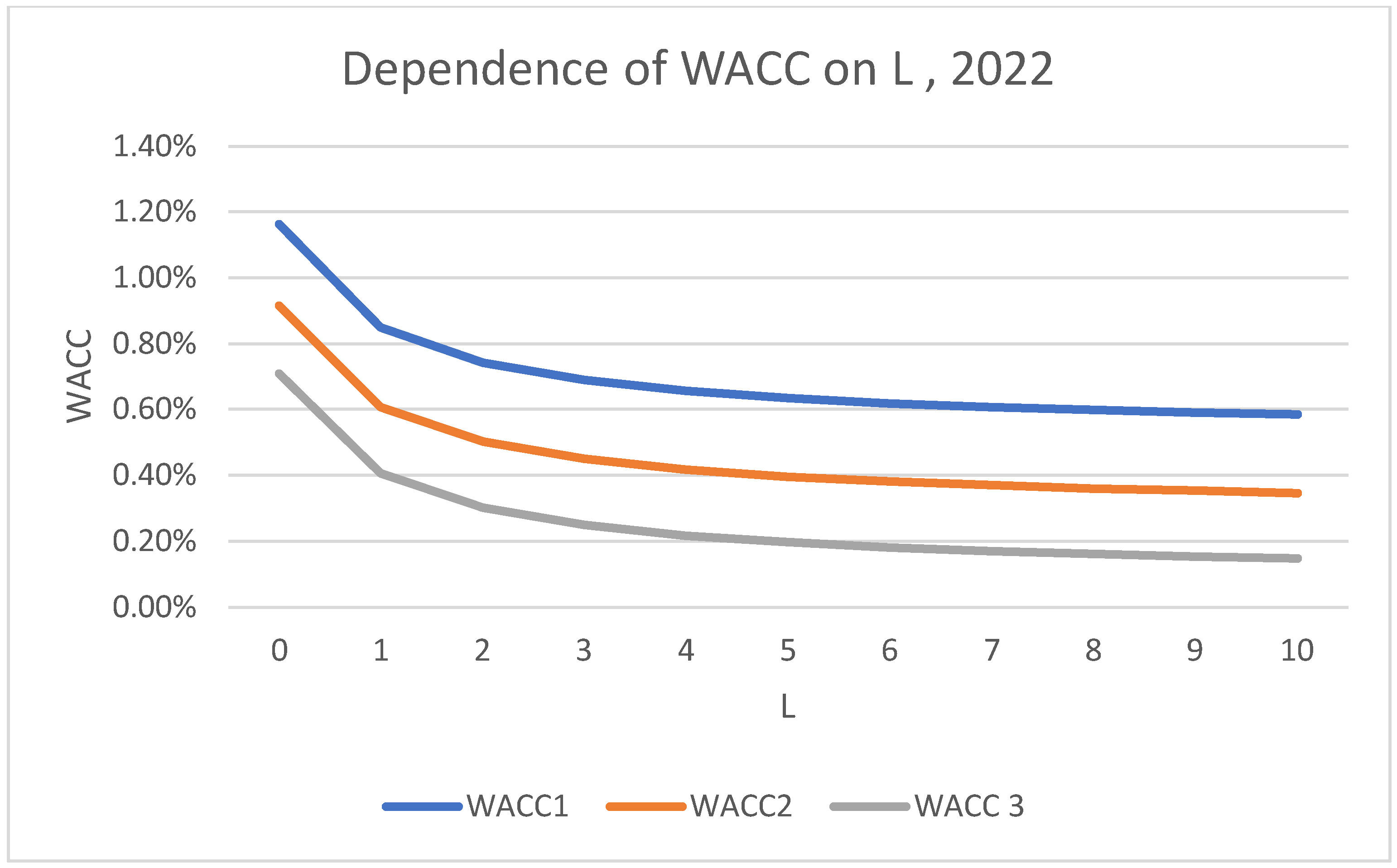
5.1. The Dependence of WACC on the Leverage

Next, let us calculate the dependence of WACC on the leverage of the company (

Table 4. WACC dependence on L (n is fixed).

	2020			2021			2022			2023
L	WACC1	WACC2	WACC3	WACC1	WACC2	WACC3	WACC1	WACC2	WACC3	WACC1	WACC2	WACC3
0	4.22%	4.60%	4.19%	0.78%	0.86%	0.77%	1.16%	0.92%	0.71%	4.66%	4.39%	2.61%
1	3.79%	4.16%	3.76%	0.48%	0.56%	0.47%	0.85%	0.61%	0.40%	4.21%	3.95%	2.21%
2	3.64%	4.01%	3.61%	0.37%	0.46%	0.37%	0.74%	0.50%	0.30%	4.06%	3.80%	2.07%
3	3.57%	3.94%	3.54%	0.32%	0.41%	0.31%	0.69%	0.45%	0.25%	3.98%	3.72%	2.01%
4	3.53%	3.89%	3.49%	0.29%	0.37%	0.28%	0.66%	0.42%	0.22%	3.93%	3.68%	1.97%
5	3.50%	3.86%	3.47%	0.27%	0.35%	0.26%	0.63%	0.40%	0.20%	3.90%	3.64%	1.94%
6	3.48%	3.84%	3.44%	0.25%	0.34%	0.25%	0.62%	0.38%	0.18%	3.88%	3.62%	1.92%
7	3.46%	3.83%	3.43%	0.24%	0.33%	0.24%	0.61%	0.37%	0.17%	3.86%	3.61%	1.90%
8	3.45%	3.81%	3.42%	0.24%	0.32%	0.23%	0.60%	0.36%	0.16%	3.85%	3.59%	1.89%
9	3.44%	3.80%	3.41%	0.23%	0.31%	0.22%	0.59%	0.35%	0.15%	3.84%	3.58%	1.88%
10	3.43%	3.79%	3.40%	0.22%	0.31%	0.21%	0.58%	0.35%	0.15%	3.83%	3.58%	1.87%

) based on the Brusov–Filatova–Orekhova theory for three values of k₀ for 2020–2023 years:

$${\displaystyle \frac{1-{\left(1+WACC\right)}^{-n}}{WACC}}={\displaystyle \frac{1-{\left(1+k_0\right)}^{-n}}{\left(k_0\right)\cdot \left(1-w_{d}t\left[1-{\left(1+k_d\right)}^{-n}\right]\right)}}$$

(30)

As we can see from Table 4 above, WACC always decreases with L.

Below, we provide the Figure 2, Figure 3 and Figure 4 for 2020–2023 years.

WACC1 corresponds to the case of financial risk without business risk; WACC2 accounting financial risk along with industry business risk; WACC3 accounting financial risk along with market business risk. The ordering of dependencies WACC(L) is as follows (from big values to small ones): 213.

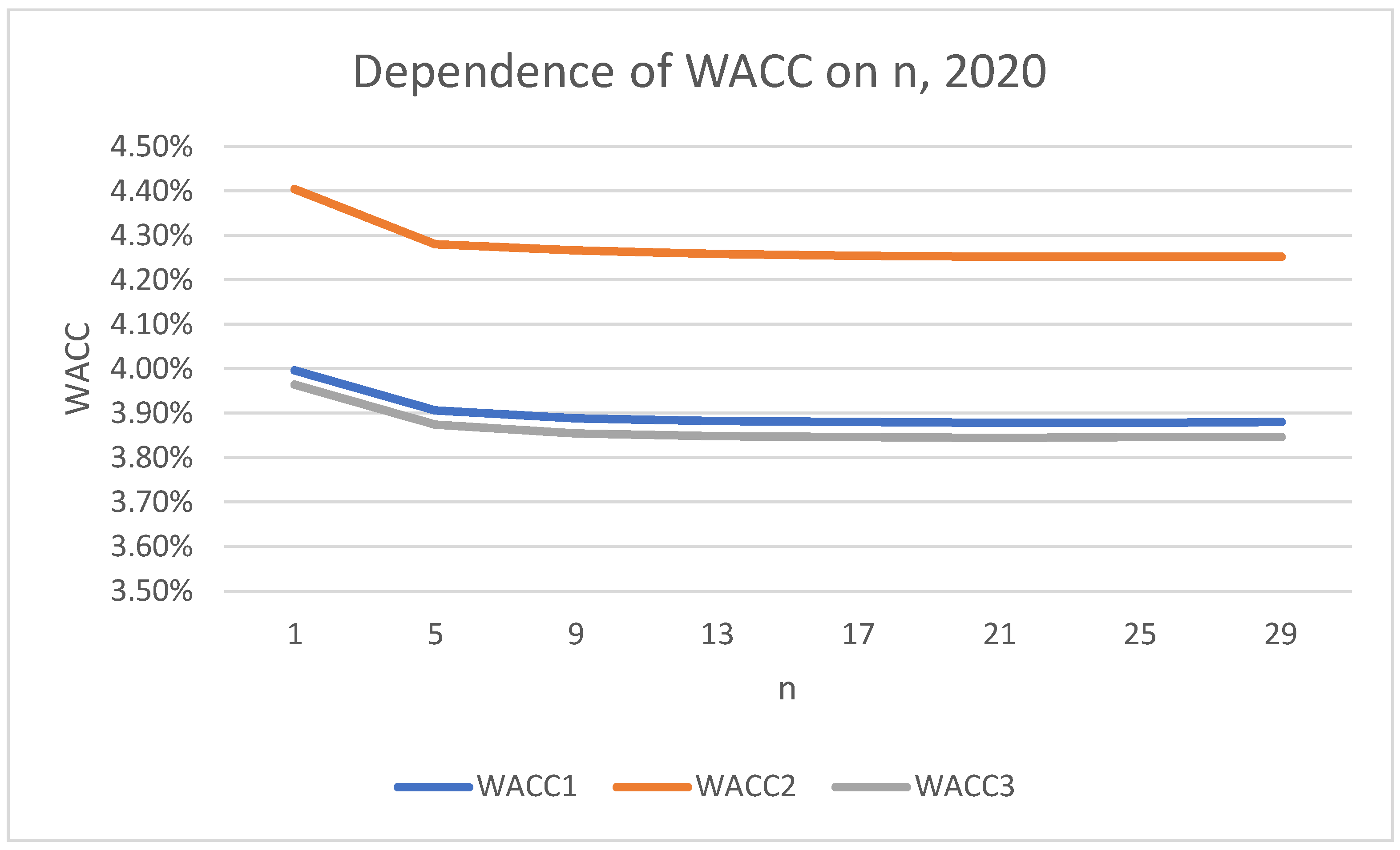
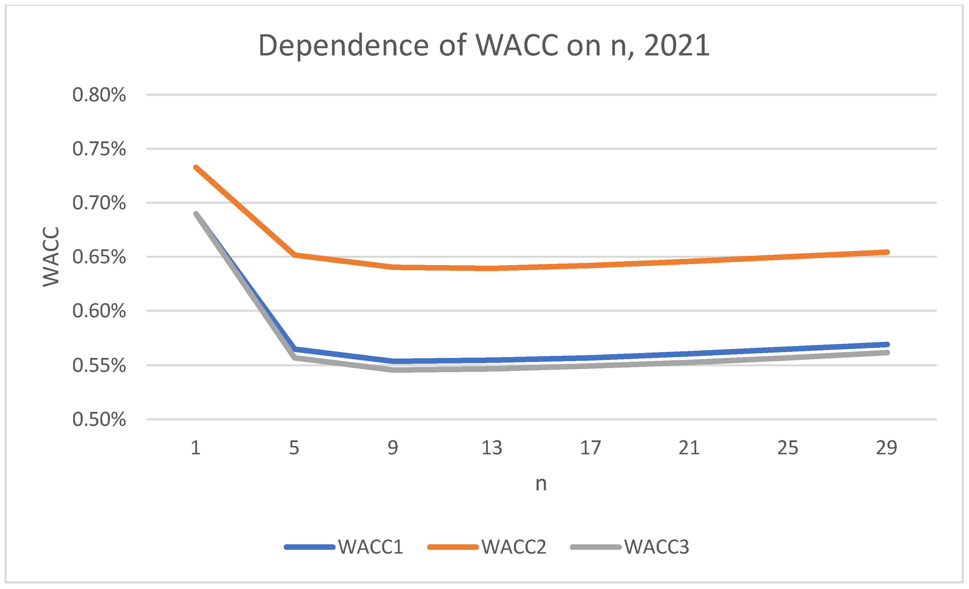
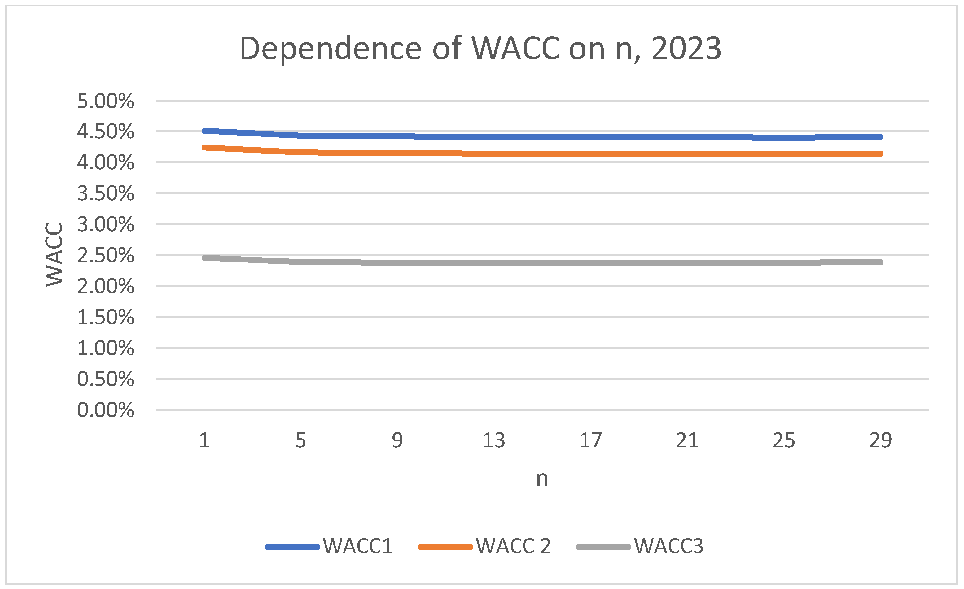
5.2. Dependence of WACC on Company Age n

Within the framework of the new approach we developed, calculating the dependence of WACC on the age of the company n plays a decisive role in assessing the business and the value of the company. Below we calculate the dependence of WACC on the company’s age (

Table 5. WACC dependence on n (L is fixed).

	2020			2021			2022			2023
n	WACC1	WACC2	WACC3	WACC1	WACC2	WACC3	WACC1	WACC2	WACC 3	WACC1	WACC 2	WACC3
1	4.00%	4.41%	3.96%	0.69%	0.73%	0.69%	1.00%	0.77%	0.57%	4.52%	4.25%	2.47%
5	3.91%	4.28%	3.87%	0.56%	0.65%	0.56%	0.93%	0.69%	0.48%	4.43%	4.16%	2.39%
9	3.89%	4.27%	3.85%	0.55%	0.64%	0.55%	0.92%	0.67%	0.47%	4.42%	4.15%	2.38%
13	3.88%	4.26%	3.85%	0.55%	0.64%	0.55%	0.92%	0.67%	0.47%	4.41%	4.15%	2.38%
17	3.88%	4.25%	3.85%	0.56%	0.64%	0.55%	0.92%	0.68%	0.47%	4.41%	4.14%	2.38%
21	3.88%	4.25%	3.85%	0.56%	0.65%	0.55%	0.92%	0.68%	0.48%	4.41%	4.14%	2.38%
25	3.88%	4.25%	3.85%	0.56%	0.65%	0.56%	0.93%	0.68%	0.48%	4.41%	4.14%	2.38%
29	3.88%	4.25%	3.85%	0.57%	0.65%	0.56%	0.93%	0.69%	0.49%	4.41%	4.14%	2.39%

). Since the age of Amazon in 2023 is 29 years, we take ages from 1 to 29 with a 4-year interval.

Table 5 above shows that WACC decreases with the company’s age. We can note that in both calculations (Table 4 and Table 5), there is a notable drop in 2021–2022 due to the aforementioned COVID-19 pandemic’s effects and several other circumstances including growing competition and regulatory changes.

Below, we show figures for the dependence of WACC on company’s age n for 2020–2023 years.

As we can see from Figure 5, Figure 6, Figure 7, Figure 8 and Figure 9, WACC decreases with n.

6. Company’s Capitalization and Business Valuation

Finally, we calculate the company’s capitalization and make a business valuation for Amazon company in 2023. For business valuation, we use two different time horizons for the representative period (5 years and 10 years) (

Table 6. Capitalization of Amazon at L as of 2023, USD thousand.

	k0 (1)	k0 (2)	k0 (3)
Vn1	596,506.73	615,285.46	764,800.40
V12 (5 years)	162,180.55	163,392.88	171,760.79
V12 (10 years)	292,876.89	296,758.25	324,403.42
V23 (WACC for 2028)	838,145.17	892,128.24	1,549,305.55
V23 (WACC for 2033)	840,663.39	894,921.14	1,554,781.56
V13 (5 years)	838,080.23	892,063.63	1,549,258.37
V13 (10 years)	840,265.88	894,523.37	1,554,480.47

and

Table 7. The current Amazon company’s capitalization (for 2023).

	k0 (1)	k0 (2)	k0 (3)
WACC	4.41%	4.14%	2.39%
Vn1	596,506.73	615,285.46	764,800.40
(1 + WACC)29	3.496	3.243	2.0164
V	2,085,387.528	1,995,370.747	1,542,143.527

).

6.1. Company’s Capitalization

In Table 7, we show the results of calculation of the current Amazon company’s capitalization (for 2023).

To calculate the current Amazon company’s capitalization (for 2023), we should accrual V_n1 for 29 periods, using the following formula:

V= V_n1 (1 + WACC)²⁹

Market capitalization of the Amazon company (as any other listed company) represents the total value of a public company’s outstanding shares and is calculated by multiplying the current share price by the total number of shares outstanding. The actual value of the Amazon company V on 30 December 2023 is equal to USD 1.57 trillion.

Comparing the results of our calculations of Amazon’s capitalization for three values of k₀ with this actual value (USD 1.57 trillion), we conclude that the best result is the one that takes into account market business risk along with financial risk, described by the BFO theory.

Note as well that accounting for only financial risk gives the biggest difference between Amazon’s actual value (USD 1.57 trillion) and calculated (USD 2.085 trillion) and less difference under the accounting of industry business risk (USD 1.995 trillion).

To test the above conclusion that the best result for Amazon’s capitalization is the one that takes into account market business risk along with financial risk, describing it with the BFO theory, we calculate below (see

Table 8. Capitalization of Amazon company V within CAPM and CAPM 2.0 approaches.

		CAPM	CAPM 2.0
Industry	Profitability μ	3.56%	4.14%
	V (mln USD)	1,819,661.62	2,035,379.43
Market	$\beta$	1.41%	2.1%
	V (mln USD)	1,309,078.94	1,451,325.72

) Amazon’s capitalization within the CAPM itself (taking into account business risk only) and CAPM 2.0 (taking into account business risk and our adjustments for non-zero leverage, but without using the WACC approach) and compare the obtained results with the market capitalization of Amazon V on 12/30/2023, which is equal to USD 1.57 trillion. For calculations, we use the data from Table 2 and CF for 2023 is equal to USD 36,852 million).

Table 8 shows that the industry approach always overestimates capitalization, and in the case of CAPM 2.0, the difference is greater. But with the market approach, CAPM 2.0 yields a better result compared to CAPM (the difference changes from USD 26 billion to USD 11.9 billion). Based on the calculations performed and comparison of the results obtained with market capitalization of Amazon, the following global conclusions can be drawn.

1. Neither CAPM nor WACC by themselves can correctly calculate a company’s capitalization.

2. At the same time within the CAPM model, the market approach turns out to be more accurate than the industry approach.

3. The best outcome is one that considers market business risk along with the financial risk described by the BFO theory.

These findings are very important and should be used in business valuation, which is discussed in the next paragraph.

6.2. Business Valuation

The DCF method does rely on forecasting future cash flows. A modification of the BFO theory (and also the MM theory) has been developed by the authors for the case of variable income. It is possible to use the company’s cash flow data for the past three to five years to determine the growth rate, and then forecast the cash flow for a representative (terminate) period.

Below, we evaluate the Amazon company using two different time horizons for the representative period, 5 years and 10 years, as is customary within the assessment procedure. We take leverage level L as the average for 4 years (2020–2023).

One can see from

Table 9. V_n1, V₁₂, V₂₃, V₁₃ of Amazon at L as the average, USD thousand.

	k0 (1)	k0 (2)	k0 (3)
Vn1	601,050.96	619,970.11	770,608.32
V12 (5 years)	162,477.89	163,688.72	172,047.85
V12 (10 years)	293,825.97	297,710.14	325,378.46
V23 (WACC for 2028)	848,016.72	902,893.07	1,577,654.36
V23 (WACC for 2033)	847,974.01	902,722.77	1,573,830.32
V13 (5 years)	848,017.07	902,898.39	1,577,682.23
V13 (10 years)	847,978.28	902,751.28	1,574,020.84

that Amazon company valuation is equal to USD 0.848 trillion under accounting financial risk only, USD 0.903 trillion under accounting industry business risk along with financial risk and USD 1.574 trillion under accounting market business risk along with financial risk.

Using our experience above with an estimation of Amazon company value, we conclude that the best result is the one that takes into account market business risk along with financial risk, described by the BFO theory. Thus, the Amazon company valuation for the end of 2023 is equal to USD 1.574 trillion.

7. Conclusions

A new approach to business valuation and company value has been developed. Two of the three approaches to the income method have been modified: CAPM and WACC. When modifying CAPM, a new model, CAPM 2.0, was created, within which business and financial risks were simultaneously taken into account. Moreover, for the first time, this was performed correctly and the inaccuracy, incorrectness and inconsistency of the popular Hamada model were shown. When modifying the WACC approach (or the discounted income method), the real operating conditions of companies were taken into account. The use of the modern theory of capital structure (the Brusov–Filatova–Orekhova (BFO) theory) allows one to correctly determine the main valuation parameter—the discount rate—and link the retrospective terminate periods with the representative one. The application of the new methodology to one of the first-class companies (Amazon (AMZN)) is considered. We calculate both Amazon’s capitalization and business valuation.

Based on the capitalization calculations and comparison of the results with Amazon’s market capitalization, the following conclusions can be drawn:

1. Neither CAPM nor WACC can correctly calculate a company’s capitalization by themselves.

2. At the same time, within the CAPM model, the market approach is more accurate than the industry approach.

3. The best result is the one that takes into account market business risk together with the financial risk described by the BFO theory.

These conclusions are very important and should be used in business valuation.

For companies with variable income, the BFO theory modified for this case should be used. In this case, as it has been shown (Brusov et al., 2023; Brusov and Filatova, 2024) [3,4] (see Formulas (27)–(29)), not only the profitability, CF, but also the discount rate WACC depends on the growth rate g. Thus, in this (quite common) case, it becomes possible to correctly predict both the valuation of the business and the value of the company.

In this case, it is necessary to collect data on the company’s financial income for the last 3–5 years and, on their basis, determine the growth rate g of the company’s income.

Knowing the growth rate, using the BFO formula for WACC with variable income, we can make a forecast for both the representative period and the terminate one. The latter can be finite (say 10 years) or infinite. In the latter case, the MM formula for company value should be used.

The new methodology increases significantly the accuracy of the valuation. The closeness of the new methodology’s results to the Amazon company (AMZN) actual market value (calculated by trivially multiplying the current share price by the total number of shares outstanding) shows the importance and validity of this methodology, which should be applied to business valuation.

The developed methodology allows us to combat the main drawback of existing evaluation methods—the impossibility or serious difficulties in the correct evaluation of the main evaluation parameter—the discount rate. The correct determination of the discount rate will help to prevent abuses in business evaluation, in investments, in determining the fair value of shareholders’ dividend income.

8. Some Notes on Remaining Issues and Future Directions of Work

The size of the company matters and should be taken into account as an additional premium to the discount rate. Such additional adjustments are taken into account in several theories, for example, in the five-factor model of Fama and French and in the Sharpe model. To account for enterprises in other sectors, the industry approach described in the developed methodology should be used.

The DCF method does rely on forecasting future cash flows. A modification of the BFO theory (and also the MM theory) has been developed by the authors for the case of variable income. It is possible to use the company’s cash flow data for the past three to five years to determine the growth rate, and then forecast the cash flow for a representative (terminate) period.

Recently, the WACC formulas within the framework of the Brusov–Filatova–Orekhova (BFO) theory and the Modigliani–Miller (MM) theory have been modified, taking into account the conditions of the actual operation of the company, such as frequent payment of income tax, the method of paying income tax (at the end of periods or in advance), etc. To improve the accuracy of business valuation, it is necessary to take these effects into account.

Macroeconomic uncertainties, such as interest rate changes or geopolitical risks, must be taken into account. In the presented methodology, they are taken into account only to the extent that they are taken into account in the market business risk. A more accurate accounting of these risks requires additional assessment and accounting in the form of a premium to the discount rate. Similarly, country risk and specific risk associated with a particular company must be taken into account.