Strongly Coupled Designs for Computer Experiments with Both Qualitative and Quantitative Factors

Abstract

Computer experiments often involve both qualitative and quantitative factors, posing challenges for efficient experimental designs. Strongly coupled designs (SCDs) are proposed in this paper to balance flexibility in run size and stratification properties between qualitative and quantitative factor columns. The existence and construction of SCDs are investigated. When $s⩾2$ is a prime or a prime power, the constructed SCDs of $\lambda s^3$ runs can accommodate $2s-1$ qualitative factors and a substantial number of quantitative factors. Furthermore, a series of SCDs with $s^u$ rows and $(u-3)s^3$ columns of quantitative factors are constructed, where $u⩾4$, with certain columns of quantitative factors achieving stratification in two or higher dimensions. The proposed SCDs achieve stratification between any two qualitative factors and all quantitative factors, which is superior to MCDs. With the number of levels of the qualitative factors given as $s^2$, DCDs have $\lambda s^4$ rows, while SCDs have only $\lambda s^3$ rows, offering more flexibility. Furthermore, in the designs constructed in this paper with fewer than 100 rows, in 11 out of 17 cases, SCDs have a larger number and higher levels of qualitative factors than DCDs.

1. Introduction

With the rapid development of computer science, an increasing number of scientists and engineers are using computer experiments to study complex physical systems. Space-filling designs are feasible for these types of experiments as they spread the design points in the design region as uniformly as possible (Santner, Williams and Notz, 2003; Fang, Li and Sudjianto, 2006)  [1,2]. Based on the effect sparsity principle (Wu and Hamada, 2021) [3], only a few factors are expected to be active, which makes it reasonable to focus on uniformity properties in low-dimensional projections. Latin hypercube designs (LHDs), which are among the most popular space-filling designs, satisfy one-dimensional uniformity (McKay, Beckman and Conover, 1979) [4]. Owen (1992) and Tang (1993) [5,6] proposed two methods to generate LHDs based on orthogonal arrays (OAs), which inherit t-dimensional projection properties when an OA of strength t is used. He and Tang (2013) [7] proposed a new class of arrays called strong orthogonal arrays (SOAs). To achieve better stratification properties, the strength of SOAs should be 3 or higher (He and Tang, 2014) [8], though this can lead to large run sizes. SOAs of strengths of $2+$, introduced by He, Cheng and Tang (2018) [9], are more economical than SOAs of strength 3 while retaining the same two-dimensional stratification. Zhou and Tang (2019) [10] proposed SOAs of strength $3-$, which maintain the same three-dimensional stratification as SOAs of strength 3, as well as the same factor levels as SOAs of strength 2. Recent studies on the construction of designs achieving stratification in low dimensions also include those of Liu et al. (2024), and Wang, Lin and Liu (2024) [11,12].

In some cases, computer experiments involve both quantitative and qualitative factors. Qian, Wu and Wu (2008) [13] proposed a Gaussian process model framework to address the integration of qualitative and quantitative factors in computer modeling. This framework achieves integration by constructing and validating correlation functions that incorporate both types of factors. Han et al. (2009) [14] proposed a Bayesian methodology for predicting computer experiments with both qualitative and quantitative inputs, modeling outputs for different qualitative levels as having similar functional behavior in the quantitative inputs. Huang et al. (2016) [15] introduced SLHDs with good uniformity for each slice and an adaptive analysis strategy to improve prediction precision and assess similarities among qualitative variable levels in computer experiments.

Qian (2012) [16] suggested sliced LHDs (SLHDs) for this type of experiment. Recently, Kumar et al. (2024) [17] investigated the construction methods for sliced orthogonal LHDs with unequal batch sizes. Guo et al. (2023) [18] proposed methods for constructing orthogonal and nearly orthogonal general SLHDs; these designs ensure orthogonality not only in the overall design but also within each layer before and after collapsing. Wang, Wang and Xue (2023) [19] proposed a sequential optimal LHD method to improve the space-filling properties of two-layer computer simulators. In SLHDs, stratification is achieved between all qualitative and quantitative factors; however, this can lead to a significant increase in the run sizes as the number and levels of qualitative factors expand. To provide more economical run sizes, Deng, Hung and Lin (2015) [20] proposed marginally coupled designs (MCDs). Subsequently, a large number of researchers have contributed to the study of MCDs with better properties, such as orthogonality or low-dimensional stratification, including He, Lin and Sun (2017); He et al. (2017); He, Lin and Sun (2019); and Zhou, Yang and Liu (2021) [21,22,23,24]. To study the interaction of the qualitative and quantitative factors, Yang et al. (2023) [25] proposed doubly coupled designs (DCDs) and studied their constructions. DCDs employ better stratification properties between qualitative and quantitative factors compared to MCDs, though this comes at the cost of reducing the number of qualitative factors. Zhou, Huang and Li (2024) [26] investigated the construction of group DCDs.

In this paper, a new type of design called strongly coupled designs (SCDs) is proposed for computer experiments with both quantitative and qualitative factors. Similar to DCDs, SCDs achieve stratification between any two qualitative factors and all quantitative factors to a certain extent. Compared to MCDs, SCDs are more feasible for studying interactions between any two qualitative factors and all quantitative factors. The stratification requirements among qualitative factors are relaxed which makes the run sizes of SCDs more flexible than those of DCDs. For example, when the levels of the qualitative factors are $s^2$, DCDs divide the design corresponding to the quantitative factors into $s^4$ small LHDs, with each corresponding to a specific level combination of two qualitative factors, while SCDs divide it into $s^3$ small LHDs.

The characteristics and construction methods of SCDs are also studied. The necessary and sufficient conditions for the existence of SCDs are provided from three different perspectives, and SCDs with $\lambda s^3$ runs, where $s⩾2$ is a prime or a prime power, and $\lambda$ is a positive integer, are constructed. For a given run size, the constructed SCDs can accommodate a greater number of qualitative factors than DCDs in many cases. Additionally, the construction of SCDs with desirable space-filling properties for quantitative factors is investigated. A series of designs with $s^u$ runs and $(u-3)s^3$ columns of quantitative factors, where $u⩾4$, are constructed. In these designs, certain quantitative factor columns achieve stratification in two or more dimensions.

The remainder of this paper is organized as follows. In Section 2, some basic concepts are introduced, SCDs are defined, and their existence is studied. In Section 3, the construction of SCDs is explored, including those with desirable space-filling properties for quantitative factors. Examples are provided to illustrate the construction process and the properties of the resulting designs. The paper is concluded with a discussion in Section 4. Some theorem proofs are deferred to the Appendix A.

2. Definitions and Characterizations

In this section, key concepts relevant to our work are reviewed, and the definition of SCDs is proposed. Additionally, three characterizations of SCDs are presented, providing heuristic guidance for the construction methods discussed in the next section.

An $n\times m$ array, where the j-th column has $s_j$ levels, $\{0,1,\dots ,s_j-1\}$, is called an OA of strength t, denoted by $\mathrm{OA}(n,m,s_1\times \cdots \times s_m,t)$, if every $n\times t$ subarray contains each t-tuple with equal frequency. When $s_1=\cdots =s_m=s$, the array is symmetric and is denoted as $\mathrm{OA}(n,m,s,t)$ for simplicity. An $\mathrm{OA}(n,m,s,t)$ is said to be completely resolvable, denoted by $\mathrm{CROA}(n,m,s,t)$, if its rows can be partitioned into $n/s$ subarrays, each of which is an $\mathrm{OA}(s,m,s,1)$.

An $r\times e$ array $D(r,e,s)$ is called a difference scheme based on $GF\left(s\right)$ if it satisfies the following property: for all i and j such that $1⩽i,j⩽e$ and $i\ne j$, the vector difference between the i-th and j-th columns contains each element of $GF\left(s\right)$ with equal frequency. Difference schemes are fundamental in the construction of CROAs.

An SOA of strength t, denoted by $\mathrm{SOA}(n,m,s^t,t)$, is an $n\times m$ matrix with entries from $\{0,1,\dots ,s^t-1\}$. For any subarray consisting of g columns ($1⩽g⩽t$), it can be collapsed into an $\mathrm{OA}(n,g,s^{u_1}\times \cdots \times s^{u_g},g)$, where $u_1,\dots ,u_g$ are positive integers satisfying $u_1+\cdots +u_g=t$. The $s^t$ levels of a factor are collapsed into $s^{u_j}$ levels using the mapping $\lfloor a/s^{t-u_j}\rfloor$, where $a=0,1,\dots ,s^t-1$ and $1⩽j⩽g$. Here, $\lfloor b\rfloor$ denotes the greatest integer less than or equal to b. An SOA of strength $2+$, denoted by $\mathrm{SOA}(n,m,s^2,2+)$, is an $\mathrm{SOA}(n,m,s^2,2)$ with the additional property that any two distinct columns can be collapsed into both an $\mathrm{OA}(n,2,s^2\times s,2)$ and an $\mathrm{OA}(n,2,s\times s^2,2)$. Similarly, an SOA of strength $3-$, denoted by $\mathrm{SOA}(n,m,s^2,3-)$, is an $\mathrm{SOA}(n,m,s^2,2+)$ with the property that any three distinct columns can be collapsed into an $\mathrm{OA}(n,3,s,3)$.

For two matrices $E={\left(e_{ij}\right)}_{m\times n}$ and $F={\left(f_{ij}\right)}_{u\times v}$ with entries from $GF\left(s\right)$, their Kronecker sum ⊕ is defined as

$$E\oplus F=\left(\begin{array}{ccc}{e}_{11}\dot{+}F& \cdots & e_{1n}\dot{+}F\\ ⋮& \ddots & ⋮\\ e_{m1}\dot{+}F& \cdots & e_{mn}\dot{+}F\end{array}\right),$$

where $\dot{+}$ denotes addition in $GF\left(s\right)$. $1_s$ is used to denote a vector of length s consisting entirely of ones. For any vector $w={(w_1,\dots ,w_m)}^T$, $w\otimes 1_s$ is defined as ${(w_1,\dots ,w_1,w_2,\dots ,w_m)}^T$ and $1_s\otimes w$ is defined as ${(w_1,\dots ,w_m,\dots ,w_1,\dots ,w_m)}^T$.

Let $D=(D_1,D_2)$ be a design with q qualitative factors and p quantitative factors, where $D_1$ and $D_2$ are sub-designs for qualitative and quantitative factors, respectively. A design D is called an MCD if $D_2$ is an LHD and the rows in $D_2$ corresponding to each level of any factor in $D_1$ form a small LHD. A DCD is an MCD with the additional property that the rows in $D_2$ corresponding to each level combination of any two factors in $D_1$ form an LHD.

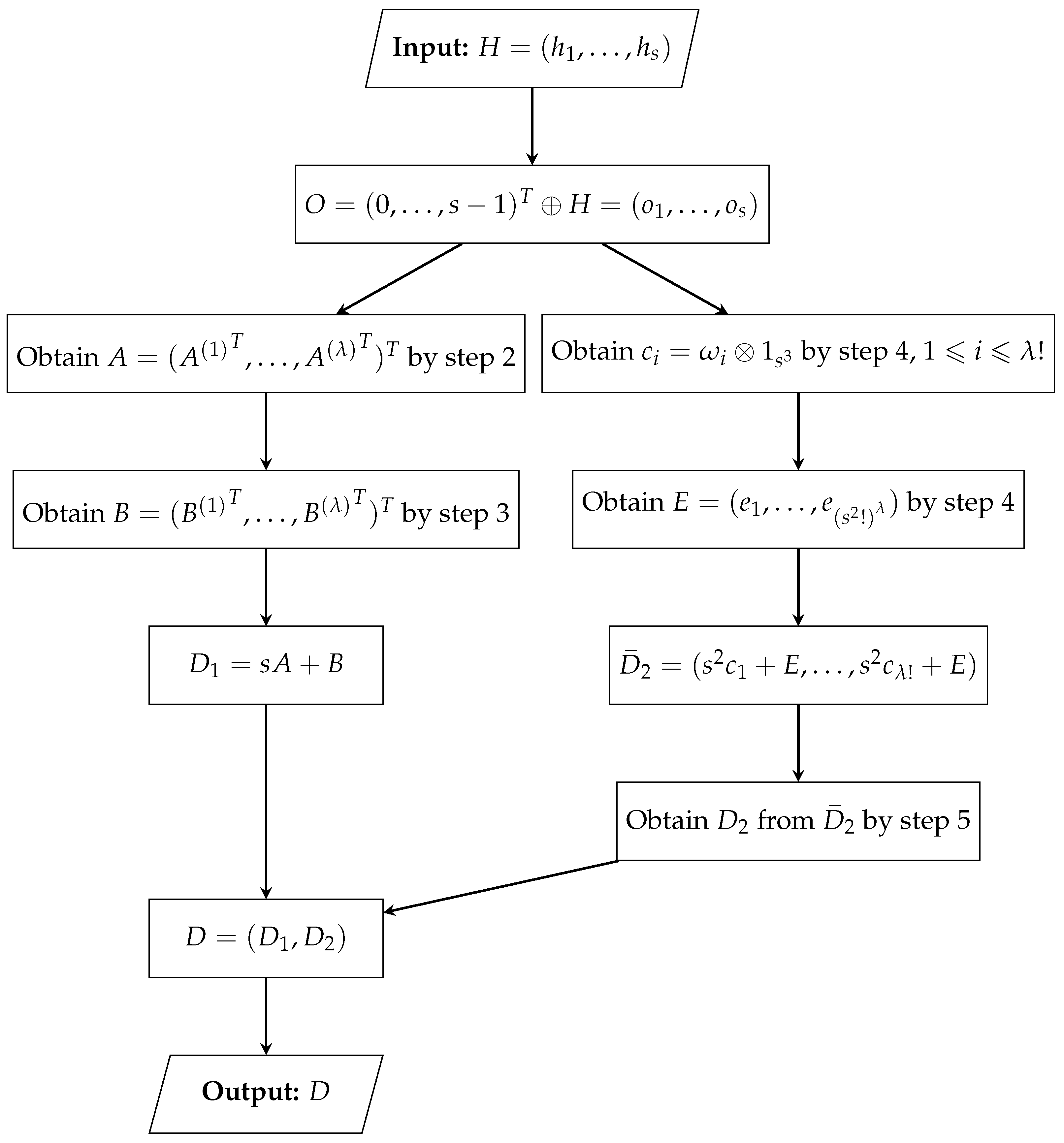
In this paper, we introduce a new class of designs for computer experiments with both quantitative and qualitative factors. Suppose the $s^2$ levels of any qualitative factor are divided into s groups based on a specified grouping method, with each group labeled by a group number: 0, 1, ..., $s-1$. The definition of SCDs is presented below.

Definition 1.

An n-run design $D=(D_1,D_2)$, with q $s^2$-level qualitative factors and p quantitative factors, is called a strongly coupled design, denoted by $\mathrm{SCD}(n,{\left(s^2\right)}^q,p)$, if it satisfies the following conditions:

(i)  

$D_2$ is an LHD;

(ii) 

The rows in $D_2$ corresponding to each group number of any column in $D_1$ form an LHD;

(iii)

The rows in $D_2$ corresponding to each combination of group number and level from any two columns in $D_1$ form an LHD.

For $D_1=(z_1,\dots ,z_q)$, to simplify the following discussion, the $s^2$ levels of qualitative factors are encoded as $0,1,\dots ,s^2-1$. The group number is defined as ${\overline{z}}_i=\lfloor {\displaystyle \frac{z_i}{s}}\rfloor$, which is obtained by collapsing the $s^2$ levels into s levels, with levels sharing the same group number classified into the same group. In this paper, $D_1$ is set as an $\mathrm{SOA}(n,q,s^2,2+)$. For $D_2=(d_1,\dots ,d_p)$, define

$${\overline{D}}_2=\lfloor {\displaystyle \frac{D_2}{s}}\rfloor =({\overline{d}}_1,\dots ,{\overline{d}}_p) \mathrm{and} {\tilde{D}}_2=\lfloor {\displaystyle \frac{{\overline{D}}_2}{s^2}}\rfloor =({\tilde{d}}_1,\dots ,{\tilde{d}}_p),$$

where $\lfloor a\rfloor$ represents the largest integer not exceeding a.

Next, we present the necessary and sufficient conditions for the existence of SCDs. Theorem 1 specifies the conditions that must be satisfied between columns from $D_1$ and $D_2$.

Theorem 1.

Suppose $D_1=(z_1,\dots ,z_q)$ is an $\mathrm{SOA}(n,q,s^2,2+)$, and $D_2=(d_1,\dots ,d_p)$ is an $\mathrm{LHD}(n,p)$. The design $D=(D_1,D_2)$ is an $\mathrm{SCD}(n,{\left(s^2\right)}^q,p)$ if and only if:

(i) 

$({\overline{z}}_i,{\overline{d}}_k)$ is an $\mathrm{OA}(n,2,s(n/s),2)$ for any $1⩽i⩽q$, $1⩽k⩽p$;

(ii)

$(z_i,{\overline{z}}_j,{\tilde{d}}_k)$ is an $\mathrm{OA}(n,3,s^{2}s(n/s^3),3)$ for any $1⩽i\ne j⩽q$, $1⩽k⩽p$.

Assume that $D_1$ is generated by the formula $sA+B$. Theorem 2 provides the necessary and sufficient conditions that the columns of A and B must satisfy for the existence of SCDs.

Theorem 2.

Suppose that $D_1=(z_1,\dots ,z_q)$ is an $\mathrm{SOA}(n,q,s^2,2+)$ generated by $D_1=sA+B$, where $A=({\overline{z}}_1,\dots ,{\overline{z}}_q)$ and $B=(b_1,\dots ,b_q)$. The design $D=(D_1,D_2)$ is an $\mathrm{SCD}(n,{\left(s^2\right)}^q,p)$ if and only if:

(i) 

A can be divided as $({A^{\left(1\right)}}^T,\dots ,{A^{(n/s^3)}}^T{)}^T$, where each $A^{\left(l\right)}$ is a $\mathrm{CROA}(s^3,q,s,2)$, for $1⩽l⩽n/s^3$;

(ii)

For any two columns ${\overline{z}}_i^{\left(l\right)}$ and ${\overline{z}}_j^{\left(l\right)}$ in $A^{\left(l\right)}$, and the corresponding rows $b_i^{\left(l\right)}$ in $b_i$, the three tuples $({\overline{z}}_i^{\left(l\right)},{\overline{z}}_j^{\left(l\right)},b_i^{\left(l\right)})$ form an $\mathrm{OA}(n,3,s^3,3)$, for any $1⩽i\ne j⩽q$, $1⩽l⩽n/s^3$.

Assume that $D_1=sA+B$ and ${\overline{D}}_2=s^{2}C+sE+F$. Theorem 3 provides the necessary and sufficient conditions that the columns of A, B, C, E, and F must satisfy.

Theorem 3.

Suppose $D_1$ is an $\mathrm{SOA}(n,q,s^2,2+)$ and $D_2$ is an $\mathrm{LHD}(n,p)$, where $D_1$ and ${\overline{D}}_2$ are generated by $D_1=sA+B$ and ${\overline{D}}_2=s^{2}C+sE+F$, respectively. The design $D=(D_1,D_2)$ is an $\mathrm{SCD}(n,{\left(s^2\right)}^q,p)$ if and only if there exist five arrays: $A=({\overline{z}}_1,\dots ,{\overline{z}}_q)=OA(n,q,s,2)$, $B=(b_1,\dots ,b_q)=\mathrm{OA}(n,q,s,1)$, $C=({\tilde{d}}_1,\dots ,{\tilde{d}}_p)=\mathrm{OA}(n,p,n/s^3,1)$, $E=(e_1,\dots ,e_p)=\mathrm{OA}(n,p,s,1)$, and $F=(f_1,\dots ,f_q)=\mathrm{OA}(n,q,s,1)$, such that for any $1⩽i\ne j⩽q$ and $1⩽k⩽p$, both $({\overline{z}}_i,f_k,e_k,{\tilde{d}}_k)$ and $({\overline{z}}_i,b_i,{\overline{z}}_j,{\tilde{d}}_k)$ are $\mathrm{OA}(n,4,s^3(n/s^3),4)$.

3. Construction Methods

In this section, methods for constructing SCDs, as well as the ones with desirable space-filling properties for quantitative factors, are proposed. We focus on cases where $s⩾2$ is a prime or a prime power. The SCDs constructed in Section 3.1 can accommodate $2s-1$ qualitative factors and a large number of quantitative factors. For the SCDs constructed in Section 3.2, when the run size $n=s^u$, the number of columns for quantitative factors is $(u-3)s^3$, and certain columns of quantitative factors achieve stratification in two or more higher dimensions.

3.1. Construction of SCDs

SCDs with run sizes $n=\lambda s^3$ can be obtained using Algorithm 1, where $s⩾2$ is a prime or a prime power, and $\lambda$ is a positive integer.    

Algorithm 1: Construction of SCDs

Step 1. Let $H=(h_1,\dots ,h_s)$ be a $D(s,s,s)$. Define $O={(0,\dots ,s-1)}^T\oplus H=(o_1,\dots ,o_s)$, an OA obtained by developing the difference schemes H. Step 2. Define $a_1=h_1\oplus o_1$, and $A_i=(h_1,h_i)\oplus o_i$ for $i=2,\dots ,s$. Let $A^{\left(1\right)}=\cdots =A^{\left(\lambda \right)}=(a_1,A_2,\dots ,A_s)$, and $A={(A^{\left(1\right)}}^T,\dots ,{A^{\left(\lambda \right)}}^T{)}^T$. Step 3. For $1⩽j_{i,m},k_{i,m}⩽s$, where $1⩽i⩽s$, $1⩽m⩽2$, $j_{i,m}\ne k_{i,m}$ and $j_{i,m}\ne 1$, define: $b_1=h_{j_{1,1}}\oplus o_{k_{1,1}}$ with $j_{1,1}\ne 1$; $b_{i1}=h_{j_{i,1}}\oplus o_{k_{i,1}}$ with $k_{i,1}\ne 1$ and $j_{i,1}\ne i$, or $k_{i,1}=1$ and $j_{i,1}=i$; $b_{i2}=h_{j_{i,2}}\oplus o_{k_{i,2}}$ with $j_{i,2}=i$. Let $B_i=(b_{i1},b_{i2})$, and $B^{\left(1\right)}=\cdots ,B^{\left(\lambda \right)}=(b_1,B_2,\dots ,B_s)$. Then obtain $B={(B^{\left(1\right)}}^T,\dots ,{B^{\left(\lambda \right)}}^T{)}^T$. Step 4. Define $c_i={\omega }_i\otimes 1_{s^3}$, where ${\omega }_i$ is a permutation of $(0,\dots ,\lambda -1)$ for $1⩽i⩽\lambda !$. For $1⩽l⩽\lambda$ and $1⩽k⩽s^2!$, define $e_k^{\left(l\right)}=({(1_s\otimes {\beta }_{1,k}^{\left(l\right)})}^T,\dots ,{(1_s\otimes {\beta }_{s,k}^{\left(l\right)})}^T{)}^T$, where $({{\beta }_{1,k}^{\left(l\right)}}^T,\dots ,{{\beta }_{s,k}^{\left(l\right)}}^T{)}^T$ is a permutation of ${(0,\dots ,s^2-1)}^T$. For $1⩽\delta ⩽{(s^2!)}^{\lambda }$, let $e_{\delta }=({e_{k_1}^{\left(1\right)}}^T,\dots ,{e_{k_{\lambda }}^{\left(\lambda \right)}}^T{)}^T$, where $1⩽k_l⩽s^2!$. Then, obtain $E=(e_1,\dots ,e_{{(s^2!)}^{\lambda }})$. Step 5. Let $D_1=sA+B$ and ${\overline{D}}_2=(s^2{c}_1+E,\dots ,s^2{c}_{\lambda !}+E)$. For each column in ${\overline{D}}_2$, replace the s positions of level i by all possible random permutation of $\{is,is+1,\dots ,$$is+(s-1)\}$, $i=0,1,\dots ,n/s-1$, columns juxtapose these matrices to obtain $D_2$, then obtain $D=(D_1,D_2)$.

    To make it easier for readers to understand the algorithm, we provide the flow chart in Figure 1 to explain the algorithm.

Figure 1. Flow chart of Algorithm 1.

The properties of the constructed designs are summarized in the following theorem.

Theorem 4.

The design D constructed in Algorithm 1 is an $\mathrm{SCD}(n,{\left(s^2\right)}^q,p)$ with $n=\lambda s^3$, $q=2s-1$ and $p=\lambda !{(s^2!)}^{\lambda }{(s!)}^{\lambda s^2}$, where λ is a positive integer.

An example is now given to illustrate the construction procedure and the properties of the constructed designs.

Example 1.

For $s=\lambda =2$, let

$$H=(h_1,h_2)=\left(\begin{array}{cc}0& 0\\ 0& 1\end{array}\right),$$

then,

$$O={(0,1)}^T\oplus H={\left(\begin{array}{cccc}0& 0& 1& 1\\ 0& 1& 1& 0\end{array}\right)}^T=(o_1,o_2).$$

Define $a_1=h_1\oplus o_1={(0,0,1,1,0,0,1,1)}^T$,

$$A_2=(h_1,h_2)\oplus o_2={\left(\begin{array}{cccccccc}0& 1& 1& 0& 0& 1& 1& 0\\ 0& 1& 1& 0& 1& 0& 0& 1\end{array}\right)}^T,$$

then,

$$A=\left(\begin{array}{c}{A}^{\left(1\right)}\\ A^{\left(2\right)}\end{array}\right)=\left(\begin{array}{cc}{a}_1& A_2\\ a_1& A_2\end{array}\right)={\left(\begin{array}{cccccccc}0& 0& 1& 1& 0& 0& 1& 1\\ 0& 1& 1& 0& 0& 1& 1& 0\\ 0& 1& 1& 0& 1& 0& 0& 1\\ 0& 0& 1& 1& 0& 0& 1& 1\\ 0& 1& 1& 0& 0& 1& 1& 0\\ 0& 1& 1& 0& 1& 0& 0& 1\end{array}\right)}^T.$$

Define $b_1=b_{21}=b_{22}=h_2\oplus o_1={(0,0,1,1,1,1,0,0)}^T$, then,

$$B=\left(\begin{array}{c}{B}^{\left(1\right)}\\ B^{\left(2\right)}\end{array}\right)=\left(\begin{array}{cc}{b}_1& B_2\\ b_1& B_2\end{array}\right)={\left(\begin{array}{cccccccc}0& 0& 1& 1& 1& 1& 0& 0\\ 0& 0& 1& 1& 1& 1& 0& 0\\ 0& 0& 1& 1& 1& 1& 0& 0\\ 0& 0& 1& 1& 1& 1& 0& 0\\ 0& 0& 1& 1& 1& 1& 0& 0\\ 0& 0& 1& 1& 1& 1& 0& 0\end{array}\right)}^T.$$

As $\lambda =2$, let $w_1=(0,1)$ and $w_2=(1,0)$. Correspondingly, obtain

$$c_1=w_1\otimes 1_8={(0,0,0,0,0,0,0,0,1,1,1,1,1,1,1,1)}^T,$$

$$c_2=w_2\otimes 1_8={(1,1,1,1,1,1,1,1,0,0,0,0,0,0,0,0)}^T.$$

For $1⩽k⩽24$, both ${({{\beta }_{1,k}^{\left(1\right)}}^T,{{\beta }_{2,k}^{\left(1\right)}}^T)}^T$ and ${({{\beta }_{1,k}^{\left(2\right)}}^T,{{\beta }_{2,k}^{\left(2\right)}}^T)}^T$ are a permutation of ${(0,1,2,3)}^T$. Let

$$e_{\delta }=\left(\begin{array}{c}{e}_{k_1}^{\left(1\right)}\\ e_{k_2}^{\left(2\right)}\end{array}\right)={\left(\begin{array}{cc}{(1_2\otimes {\beta }_{1,k_1}^{\left(1\right)})}^T,& {(1_2\otimes {\beta }_{2,k_1}^{\left(1\right)})}^T\\ {(1_2\otimes {\beta }_{1,k_2}^{\left(2\right)})}^T,& {(1_2\otimes {\beta }_{2,k_2}^{\left(2\right)})}^T\end{array}\right)}^T,$$

for $1⩽\delta ⩽{24}^2$, $1⩽k_1,k_2⩽24$. Define $E=(e_1,\dots ,e_{{24}^2})$, then, obtain ${\overline{D}}_2=(4c_1+E,4c_2+E)$. The first 24 columns of ${\overline{D}}_2$ are listed in Table 1. The two positions of level $0,1,\dots ,7$ are replaced by all possible random permutations of $\{0,1\},\{2,3\},\dots ,\{14,15\}$, respectively. The columns of these matrices are then juxtaposed to form $D_2$.

Table 1. The SCD generated in Example 1.

${\mathit{D}}_1$				The First 24 Columns of ${\overline{\mathit{D}}}_2$
0	0	0		0	0	0	0	0	0	0	0	0	0	0	0	0	0	0	0	0	0	0	0	0	0	0	0
0	2	2		1	1	1	1	1	1	1	1	1	1	1	1	1	1	1	1	1	1	1	1	1	1	1	1
3	3	3		0	0	0	0	0	0	0	0	0	0	0	0	0	0	0	0	0	0	0	0	0	0	0	0
3	1	1		1	1	1	1	1	1	1	1	1	1	1	1	1	1	1	1	1	1	1	1	1	1	1	1
1	1	3		2	2	2	2	2	2	2	2	2	2	2	2	2	2	2	2	2	2	2	2	2	2	2	2
1	3	1		3	3	3	3	3	3	3	3	3	3	3	3	3	3	3	3	3	3	3	3	3	3	3	3
2	2	0		2	2	2	2	2	2	2	2	2	2	2	2	2	2	2	2	2	2	2	2	2	2	2	2
2	0	2		3	3	3	3	3	3	3	3	3	3	3	3	3	3	3	3	3	3	3	3	3	3	3	3
0	0	0		4	5	5	4	6	6	5	4	6	6	4	5	6	6	4	5	5	4	7	7	7	7	7	7
0	2	2		5	4	6	6	4	5	6	6	4	5	5	4	7	7	7	7	7	7	4	5	5	4	6	6
3	3	3		4	5	5	4	6	6	5	4	6	6	4	5	6	6	4	5	5	4	7	7	7	7	7	7
3	1	1		5	4	6	6	4	5	6	6	4	5	5	4	7	7	7	7	7	7	4	5	5	4	6	6
1	1	3		6	6	4	5	5	4	7	7	7	7	7	7	4	5	5	4	6	6	5	4	6	6	4	5
1	3	1		7	7	7	7	7	7	4	5	5	4	6	6	5	4	6	6	4	5	6	6	4	5	5	4
2	2	0		6	6	4	5	5	4	7	7	7	7	7	7	4	5	5	4	6	6	5	4	6	6	4	5
2	0	2		7	7	7	7	7	7	4	5	5	4	6	6	5	4	6	6	4	5	6	6	4	5	5	4

The resulting design $D=(D_1,D_2)$ is an SCD$(16,4^3,{24}^2{2}^9)$. When collapsing $D_1$ into 2 levels, the rows in $D_2$ corresponding to each level of any factor in $D_1$ form an LHD$(8,{24}^2{2}^9)$. When collapsing any two columns of $D_1$ into $4\times 2$ or $2\times 4$ levels, the rows in $D_2$ corresponding to each level combination of any two factors in $D_1$ form an LHD$(2,{24}^2{2}^9)$. Furthermore, the first two columns of $D_2$ achieve stratification on $2\times 2$ grids.

Table 2 lists various SCDs generated for different positive integer values of $\lambda$, demonstrating the flexibility of SCDs in accommodating different run sizes. Each row in the table shows the design’s ability to accommodate qualitative and quantitative factors. As the experiment size increases, the number of quantitative factors that the design can accommodate increases significantly.

Table 2. Some generated SCDs where $\lambda$ is a positive integer.

s	n	${\mathit{D}}_1$	${\mathit{D}}_2$
2	8$\lambda$	$\mathrm{SOA}(8\lambda ,3,2^2,2+)$	$\mathrm{LHD}(8\lambda ,\lambda !{(4!)}^{\lambda }{2}^{4\lambda })$
3	27$\lambda$	$\mathrm{SOA}(27\lambda ,5,2^2,2+)$	$\mathrm{LHD}(27\lambda ,\lambda !{(9!)}^{\lambda }{(3!)}^{9\lambda })$
4	64$\lambda$	$\mathrm{SOA}(64\lambda ,7,2^2,2+)$	$\mathrm{LHD}(64\lambda ,\lambda !{(16!)}^{\lambda }{(4!)}^{16\lambda })$
5	125$\lambda$	$\mathrm{SOA}(125\lambda ,9,2^2,2+)$	$\mathrm{LHD}(125\lambda ,\lambda !{(25!)}^{\lambda }{(5!)}^{25\lambda })$

Table 3 presents the comparison of SCDs, DCDs, and MCDs with the same run sizes. All three kinds of designs can accommodate a large number of qualitative factors, with MCDs supporting significantly more qualitative and quantitative factors than SCDs and DCDs. However, SCDs and DCDs outperform MCDs in terms of the stratification property between qualitative and quantitative factors. For SCDs and DCDs, in 11 out of 17 cases, SCDs have a larger number and higher levels of qualitative factors than DCDs. In the remaining cases, SCDs accommodate only one fewer qualitative factor than DCDs.

Table 3. Comparison of SCDs, DCDs, and MCDs.

n	SCD	DCD	MCD
8	SCD(8,$4^3$,$4!2^4$)	DCD(8,$2^2$,$2^{6}2!$)	MCD(8,$2^4$,$4!2^4$)
16	SCD(16,$4^3$,$2!{(4!)}^2{2}^8$)	DCD(16,$4^4$,${(4!)}^5$)	MCD(16,$4^4$,$4!{24}^4$)
24	SCD(24,$4^3$,$3!{(4!)}^3{2}^{12}$)	DCD(24,$2^2$,$2^{18}6!$)	MCD(24,$2^{12}$,$12!2^{12}$)
27	SCD(27,$9^5$,$9!{(3!)}^9$)	DCD(27,$3^3$,$6^{12}3!$)	MCD(27,$3^9$,$9!6^9$)
32	SCD(32,$4^3$,$4!{(4!)}^4{2}^{16}$)	DCD(32,$4^4$,${(4!)}^{10}2!$)	MCD(32,$4^8$,$8!{24}^8$)
40	SCD(40,$4^3$,$5!{(4!)}^5{2}^{20}$)	DCD(40,$2^2$,$2^{30}10!$)	MCD(40,$2^{20}$,$20!2^{20}$)
48	SCD(48,$4^3$,$6!{(4!)}^6{2}^{24}$)	DCD(48,$4^4$,${(4!)}^{15}3!$)	MCD(48,$4^{12}$,$12!{24}^{12}$)
54	SCD(54,$9^5$,$2!{(9!)}^2{(3!)}^{18}$)	DCD(54,$3^3$,$6^{24}6!$)	MCD(54,$3^{18}$,$18!6^{18}$)
56	SCD(56,$4^3$,$7!{(4!)}^7{2}^{28}$)	DCD(56,$2^2$,$2^{42}14!$)	MCD(56,$2^{28}$,$28!2^{28}$)
64	SCD(64,$4^3$,$8!{(4!)}^8{2}^{32}$)	DCD(64,$4^4$,${(4!)}^{20}4!$)	MCD(64,$4^{16}$,$16!{24}^{10}$)
72	SCD(72,$4^3$,$9!{(4!)}^9{2}^{36}$)	DCD(72,$3^3$,$6^{32}8!$)	MCD(72,$3^{24}$,$24!6^{24}$)
80	SCD(80,$4^3$,$10!{(4!)}^{10}{2}^{40}$)	DCD(80,$4^4$,${(4!)}^{25}5!$)	MCD(80,$4^8$,$20!{24}^{20}$)
81	SCD(81,$9^5$,$3!{(9!)}^3{(3!)}^{27}$)	DCD(81,$3^3$,$6^{36}9!$)	MCD(81,$3^{27}$,$27!6^{27}$)
88	SCD(88,$4^3$,$11!{(4!)}^{11}{2}^{44}$)	DCD(88,$2^2$,$2^{66}22!$)	MCD(88,$2^{44}$,$44!2^{44}$)
96	SCD(96,$4^3$,$12!{(4!)}^{12}{2}^{48}$)	DCD(96,$4^4$,${(4!)}^{30}6!$)	MCD(96,$4^{16}$,$24!{24}^{24}$)

3.2. Construction of SCDs with Desirable Space-Filling Properties

This section focuses on constructing SCDs in which $D_2$ has desirable space-filling properties. A series of designs with $s^u$ rows and $(u-3)s^3$ columns of quantitative factors are constructed for $u⩾4$. These designs ensure that certain columns of quantitative factors achieve stratification in two or higher dimensions.

Let ${\xi }_1,\dots ,{\xi }_u$ represent u independent columns with entries from $GF\left(s\right)$, each of length $n=s^u$. A regular saturated OA can be constructed by first listing these independent columns and then adding all possible interactions. This design is denoted as $S=\{u_1{\xi }_1+\cdots +u_u{\xi }_u\mid u_i\in GF\left(s\right),(u_1,\dots ,u_u)\ne (0,\dots ,0),\mathrm{and}\mathrm{the}\mathrm{first}\mathrm{nonzero}\mathrm{entry}\mathrm{is}1\}$. Subsequently, select columns from S to construct SCDs in which $D_2$ possesses desirable space-filling properties. For when $s⩾3$ is a prime or a prime power, we propose our construction method in Algorithm 2.

Algorithm 2: Construction of SCDs with desirable space-filling properties

Step 1. Define $A_1=\{{\xi }_1+(s-1){\xi }_2+w{\xi }_3\mid 1⩽w⩽s-2\}$ and $A_2=\{{\xi }_1+w{\xi }_2+(s-1){\xi }_3$ $\mid 1⩽w⩽s-2\}$. Construct $$A=({\xi }_1+(s-1){\xi }_2,{\xi }_2+(s-1){\xi }_3,A_1,A_2,{\xi }_1+(s-1){\xi }_2+(s-1){\xi }_3).$$ Step 2. Repeat ${\xi }_2$ and ${\xi }_3$$s-2$ times to form $B_1=({\xi }_2,\dots ,{\xi }_2)$ and $B_2=({\xi }_3,\dots ,{\xi }_3)$, respectively. Let $B=({\xi }_1,{\xi }_2,B_1,B_2,{\xi }_1)$. Construct $D_1=sA+B$. Step 3. Define $E=({\xi }_1+(s-1){\xi }_2,\dots ,{\xi }_1+(s-1){\xi }_2)$ and $F=({\xi }_1,\dots ,{\xi }_1)$, where ${\xi }_1+(s$ $-1){\xi }_2$ and ${\xi }_1$ are each repeated $(u-3)s^3$ times. Step 4. Let $R_v=\{{\xi }_1+u_2{\xi }_2+u_3{\xi }_3+u_{v+3}{\xi }_{v+3}|u_2,u_3\in GF\left(s\right),u_{v+3}\in GF\left(s\right)\setminus \left\{0\right\}\}\cup \{{\xi }_2+$ $u_3{\xi }_3+u_{v+3}{\xi }_{v+3}|u_3\in GF\left(s\right),u_{v+3}\in GF\left(s\right)\setminus \left\{0\right\}\}\cup \{{\xi }_3+u_{v+3}{\xi }_{v+3}|u_{v+3}\in GF\left(s\right)\setminus$ $\left\{0\right\}\}\cup \left\{{\xi }_{v+3}\right\}=(r_{v,1},\dots ,r_{v,s^3})$, where $1⩽v⩽u-3$. Define $$T=\left(\begin{array}{ccccc}{s}^{u-4}& 1& \cdots & s^{u-6}& s^{u-5}\\ s^{u-5}& s^{u-4}& \cdots & s^{u-7}& s^{u-6}\\ ⋮& ⋮& \ddots & ⋮& ⋮\\ s& s^2& \cdots & s^{u-4}& 1\\ 1& s& \cdots & s^{u-5}& s^{u-4}\end{array}\right)=(t_1,\dots ,t_{u-3}).$$ Let $C=(C_1,\dots ,C_{s^3})$, where $$C_f=(r_{1,f},\dots ,r_{u-3,f})T,1⩽f⩽s^3.$$ Step 5. Construct ${\overline{D}}_2=s^{2}C+sE+F$. For each column of ${\overline{D}}_2$, replace the s positions of level i with a random permutation of $\{is,is+1,\dots ,is+(s-1\left)\right\}$ to obtain $D_2$, where $i=0,1,\dots ,s^2-1$. Finally, let $D=(D_1,D_2)$.

A flow chart is provided in Figure 2 to explain the algorithm.

Figure 2. Flow chart of Algorithm 2.

For $s=2$, SCDs with desirable space-filling properties can be constructed by modifying Algorithm 2 as follows: set $A=({\xi }_1,{\xi }_1+{\xi }_2)$, $B=({\xi }_1+{\xi }_2+{\xi }_3,{\xi }_1+{\xi }_3)$, $E=({\xi }_2,\dots ,{\xi }_2)$, and $F=({\xi }_1+{\xi }_3,\dots ,{\xi }_1+{\xi }_3)$, where ${\xi }_2$ and ${\xi }_1+{\xi }_3$ are repeated $(u-3)s^3$ times. The properties of the resulting designs for $s⩾2$, where s is a prime or a prime power, are summarized in Theorem 5.

Theorem 5.

For $s⩾2$, where s is a prime or a prime power, and $u⩽4$, the design D constructed above is an $\mathrm{SCD}(s^u,{\left(s^2\right)}^q,(u-3)s^3)$ with the following properties:

(i)

$$q=\left\{\begin{array}{cc}2,\hfill & when s=2,\hfill \\ 2s-1,\hfill & when s⩾3 is a prime or a prime power;\hfill \end{array}\right.$$

(ii) 

For any m columns ${\tilde{d}}_{i_1},\dots ,{\tilde{d}}_{i_m}$ with $\lfloor (i_1-1)/(u-3)\rfloor =\cdots =\lfloor (i_m-1)/(u-3)\rfloor$, where $m⩽u-3$, the columns ${\tilde{d}}_{i_1},\dots ,{\tilde{d}}_{i_m}$ achieve stratification on $s\times \cdots \times s$ grids;

(iii)

When $\lfloor (i-1)/(u-3)\rfloor \ne \lfloor (i^{\prime }-1)/(u-3)\rfloor$, the columns ${\tilde{d}}_i$ and ${\tilde{d}}_{i^{\prime }}$ achieve stratification on $s^{u-3}\times s$ and $s\times s^{u-3}$ grids.

An example is now provided to illustrate the construction procedure and the properties of the resulting designs.

Example 2.

For $s=3$ and $u=4$, let ${\xi }_1,{\xi }_2,{\xi }_3,{\xi }_4$ be four independent columns of length $3^4$. Define $A_1={\xi }_1+2{\xi }_2+{\xi }_3$ and $A_2={\xi }_1+{\xi }_2+2{\xi }_3$. Construct

$$A=({\xi }_1,{\xi }_2,{\xi }_3)\left(\begin{array}{ccccc}1& 0& 1& 1& 1\\ 0& 1& 2& 1& 2\\ 2& 2& 1& 2& 2\end{array}\right).$$

Let $B_1={\xi }_2$ and $B_2={\xi }_3$. Then,

$$B=({\xi }_1,{\xi }_2,{\xi }_3)\left(\begin{array}{ccccc}1& 0& 0& 0& 1\\ 0& 1& 1& 0& 0\\ 0& 0& 0& 1& 0\end{array}\right).$$

Construct $D_1=sA+B$; the resulting $D_1$ is presented in Table 4.

Table 4. The generated SCD in Example 2.

${\mathit{D}}_1$						${\mathit{D}}_2$
0	0	0	0	0		0	0	0	0	0	0	0	0	0	0	0	0	0	0	0	0	0	0	0	0	0	0	0	0	0	0	0
0	0	0	0	0		9	9	9	9	9	9	9	9	9	18	18	18	18	18	18	18	18	18	9	9	9	18	18	18	9	18	9
0	0	0	0	0		18	18	18	18	18	18	18	18	18	9	9	9	9	9	9	9	9	9	18	18	18	9	9	9	18	9	18
6	6	3	7	6		0	0	0	9	9	9	18	18	18	0	0	0	9	9	9	18	18	18	0	9	18	0	9	18	9	9	0
6	6	3	7	6		9	9	9	18	18	18	0	0	0	18	18	18	0	0	0	9	9	9	9	18	0	18	0	9	18	0	9
6	6	3	7	6		18	18	18	0	0	0	9	9	9	9	9	9	18	18	18	0	0	0	18	0	9	9	18	0	0	18	18
3	3	6	5	3		0	0	0	18	18	18	9	9	9	0	0	0	18	18	18	9	9	9	0	18	9	0	18	9	18	18	0
3	3	6	5	3		9	9	9	0	0	0	18	18	18	18	18	18	9	9	9	0	0	0	9	0	18	18	9	0	0	9	9
3	3	6	5	3		18	18	18	9	9	9	0	0	0	9	9	9	0	0	0	18	18	18	18	9	0	9	0	18	9	0	18
0	4	7	3	6		6	15	24	6	15	24	6	15	24	6	15	24	6	15	24	6	15	24	15	15	15	15	15	15	6	6	6
0	4	7	3	6		15	24	6	15	24	6	15	24	6	24	6	15	24	6	15	24	6	15	24	24	24	6	6	6	15	24	15
0	4	7	3	6		24	6	15	24	6	15	24	6	15	15	24	6	15	24	6	15	24	6	6	6	6	24	24	24	24	15	24
6	1	1	1	3		6	15	24	15	24	6	24	6	15	6	15	24	15	24	6	24	6	15	15	24	6	15	24	6	15	15	6
6	1	1	1	3		15	24	6	24	6	15	6	15	24	24	6	15	6	15	24	15	24	6	24	6	15	6	15	24	24	6	15
6	1	1	1	3		24	6	15	6	15	24	15	24	6	15	24	6	24	6	15	6	15	24	6	15	24	24	6	15	6	24	24
3	7	4	8	0		6	15	24	24	6	15	15	24	6	6	15	24	24	6	15	15	24	6	15	6	24	15	6	24	24	24	6
3	7	4	8	0		15	24	6	6	15	24	24	6	15	24	6	15	15	24	6	6	15	24	24	15	6	6	24	15	6	15	15
3	7	4	8	0		24	6	15	15	24	6	6	15	24	15	24	6	6	15	24	24	6	15	6	24	15	24	15	6	15	6	24
0	8	5	6	3		3	21	12	3	21	12	3	21	12	3	21	12	3	21	12	3	21	12	21	21	21	21	21	21	3	3	3
0	8	5	6	3		12	3	21	12	3	21	12	3	21	21	12	3	21	12	3	21	12	3	3	3	3	12	12	12	12	21	12
0	8	5	6	3		21	12	3	21	12	3	21	12	3	12	3	21	12	3	21	12	3	21	12	12	12	3	3	3	21	12	21
6	5	8	4	0		3	21	12	12	3	21	21	12	3	3	21	12	12	3	21	21	12	3	21	3	12	21	3	12	12	12	3
6	5	8	4	0		12	3	21	21	12	3	3	21	12	21	12	3	3	21	12	12	3	21	3	12	21	12	21	3	21	3	12
6	5	8	4	0		21	12	3	3	21	12	12	3	21	12	3	21	21	12	3	3	21	12	12	21	3	3	12	21	3	21	21
3	2	2	2	6		3	21	12	21	12	3	12	3	21	3	21	12	21	12	3	12	3	21	21	12	3	21	12	3	21	21	3
3	2	2	2	6		12	3	21	3	21	12	21	12	3	21	12	3	12	3	21	3	21	12	3	21	12	12	3	21	3	12	12
3	2	2	2	6		21	12	3	12	3	21	3	21	12	12	3	21	3	21	12	21	12	3	12	3	21	3	21	12	12	3	21
4	0	3	3	4		13	13	13	13	13	13	13	13	13	13	13	13	13	13	13	13	13	13	4	4	4	4	4	4	4	4	4
4	0	3	3	4		22	22	22	22	22	22	22	22	22	4	4	4	4	4	4	4	4	4	13	13	13	22	22	22	13	22	13
4	0	3	3	4		4	4	4	4	4	4	4	4	4	22	22	22	22	22	22	22	22	22	22	22	22	13	13	13	22	13	22
1	6	6	1	1		13	13	13	22	22	22	4	4	4	13	13	13	22	22	22	4	4	4	4	13	22	4	13	22	13	13	4
1	6	6	1	1		22	22	22	4	4	4	13	13	13	4	4	4	13	13	13	22	22	22	13	22	4	22	4	13	22	4	13
1	6	6	1	1		4	4	4	13	13	13	22	22	22	22	22	22	4	4	4	13	13	13	22	4	13	13	22	4	4	22	22
7	3	0	8	7		13	13	13	4	4	4	22	22	22	13	13	13	4	4	4	22	22	22	4	22	13	4	22	13	22	22	4
7	3	0	8	7		22	22	22	13	13	13	4	4	4	4	4	4	22	22	22	13	13	13	13	4	22	22	13	4	4	13	13
7	3	0	8	7		4	4	4	22	22	22	13	13	13	22	22	22	13	13	13	4	4	4	22	13	4	13	4	22	13	4	22
4	4	1	6	1		10	19	1	10	19	1	10	19	1	10	19	1	10	19	1	10	19	1	10	10	10	10	10	10	1	1	1
4	4	1	6	1		19	1	10	19	1	10	19	1	10	1	10	19	1	10	19	1	10	19	19	19	19	1	1	1	10	19	10
4	4	1	6	1		1	10	19	1	10	19	1	10	19	19	1	10	19	1	10	19	1	10	1	1	1	19	19	19	19	10	19
1	1	4	4	7		10	19	1	19	1	10	1	10	19	10	19	1	19	1	10	1	10	19	10	19	1	10	19	1	10	10	1
1	1	4	4	7		19	1	10	1	10	19	10	19	1	1	10	19	10	19	1	19	1	10	19	1	10	1	10	19	19	1	10
1	1	4	4	7		1	10	19	10	19	1	19	1	10	19	1	10	1	10	19	10	19	1	1	10	19	19	1	10	1	19	19
7	7	7	2	4		10	19	1	1	10	19	19	1	10	10	19	1	1	10	19	19	1	10	10	1	19	10	1	19	19	19	1
7	7	7	2	4		19	1	10	10	19	1	1	10	19	1	10	19	19	1	10	10	19	1	19	10	1	1	19	10	1	10	10
7	7	7	2	4		1	10	19	19	1	10	10	19	1	19	1	10	10	19	1	1	10	19	1	19	10	19	10	1	10	1	19
4	8	8	0	7		16	7	25	16	7	25	16	7	25	16	7	25	16	7	25	16	7	25	25	25	25	25	25	25	7	7	7
4	8	8	0	7		25	16	7	25	16	7	25	16	7	7	25	16	7	25	16	7	25	16	7	7	7	16	16	16	16	25	16
4	8	8	0	7		7	25	16	7	25	16	7	25	16	25	16	7	25	16	7	25	16	7	16	16	16	7	7	7	25	16	25
1	5	2	7	4		16	7	25	25	16	7	7	25	16	16	7	25	25	16	7	7	25	16	25	7	16	25	7	16	16	16	7
1	5	2	7	4		25	16	7	7	25	16	16	7	25	7	25	16	16	7	25	25	16	7	7	16	25	16	25	7	25	7	16
1	5	2	7	4		7	25	16	16	7	25	25	16	7	25	16	7	7	25	16	16	7	25	16	25	7	7	16	25	7	25	25
7	2	5	5	1		16	7	25	7	25	16	25	16	7	16	7	25	7	25	16	25	16	7	25	16	7	25	16	7	25	25	7
7	2	5	5	1		25	16	7	16	7	25	7	25	16	7	25	16	25	16	7	16	7	25	7	25	16	16	7	25	7	16	16
7	2	5	5	1		7	25	16	25	16	7	16	7	25	25	16	7	16	7	25	7	25	16	16	7	25	7	25	16	16	7	25
8	0	6	6	8		26	26	26	26	26	26	26	26	26	26	26	26	26	26	26	26	26	26	8	8	8	8	8	8	8	8	8
8	0	6	6	8		8	8	8	8	8	8	8	8	8	17	17	17	17	17	17	17	17	17	17	17	17	26	26	26	17	26	17
8	0	6	6	8		17	17	17	17	17	17	17	17	17	8	8	8	8	8	8	8	8	8	26	26	26	17	17	17	26	17	26
5	6	0	4	5		26	26	26	8	8	8	17	17	17	26	26	26	8	8	8	17	17	17	8	17	26	8	17	26	17	17	8
5	6	0	4	5		8	8	8	17	17	17	26	26	26	17	17	17	26	26	26	8	8	8	17	26	8	26	8	17	26	8	17
5	6	0	4	5		17	17	17	26	26	26	8	8	8	8	8	8	17	17	17	26	26	26	26	8	17	17	26	8	8	26	26
2	3	3	2	2		26	26	26	17	17	17	8	8	8	26	26	26	17	17	17	8	8	8	8	26	17	8	26	17	26	26	8
2	3	3	2	2		8	8	8	26	26	26	17	17	17	17	17	17	8	8	8	26	26	26	17	8	26	26	17	8	8	17	17
2	3	3	2	2		17	17	17	8	8	8	26	26	26	8	8	8	26	26	26	17	17	17	26	17	8	17	8	26	17	8	26
8	4	4	0	5		23	5	14	23	5	14	23	5	14	23	5	14	23	5	14	23	5	14	14	14	14	14	14	14	5	5	5
8	4	4	0	5		5	14	23	5	14	23	5	14	23	14	23	5	14	23	5	14	23	5	23	23	23	5	5	5	14	23	14
8	4	4	0	5		14	23	5	14	23	5	14	23	5	5	14	23	5	14	23	5	14	23	5	5	5	23	23	23	23	14	23
5	1	7	7	2		23	5	14	5	14	23	14	23	5	23	5	14	5	14	23	14	23	5	14	23	5	14	23	5	14	14	5
5	1	7	7	2		5	14	23	14	23	5	23	5	14	14	23	5	23	5	14	5	14	23	23	5	14	5	14	23	23	5	14
5	1	7	7	2		14	23	5	23	5	14	5	14	23	5	14	23	14	23	5	23	5	14	5	14	23	23	5	14	5	23	23
2	7	1	5	8		23	5	14	14	23	5	5	14	23	23	5	14	14	23	5	5	14	23	14	5	23	14	5	23	23	23	5
2	7	1	5	8		5	14	23	23	5	14	14	23	5	14	23	5	5	14	23	23	5	14	23	14	5	5	23	14	5	14	14
2	7	1	5	8		14	23	5	5	14	23	23	5	14	5	14	23	23	5	14	14	23	5	5	23	14	23	14	5	14	5	23
8	8	2	3	2		20	11	2	20	11	2	20	11	2	20	11	2	20	11	2	20	11	2	20	20	20	20	20	20	2	2	2
8	8	2	3	2		2	20	11	2	20	11	2	20	11	11	2	20	11	2	20	11	2	20	2	2	2	11	11	11	11	20	11
8	8	2	3	2		11	2	20	11	2	20	11	2	20	2	20	11	2	20	11	2	20	11	11	11	11	2	2	2	20	11	20
5	5	5	1	8		20	11	2	2	20	11	11	2	20	20	11	2	2	20	11	11	2	20	20	2	11	20	2	11	11	11	2
5	5	5	1	8		2	20	11	11	2	20	20	11	2	11	2	20	20	11	2	2	20	11	2	11	20	11	20	2	20	2	11
5	5	5	1	8		11	2	20	20	11	2	2	20	11	2	20	11	11	2	20	20	11	2	11	20	2	2	11	20	2	20	20
2	2	8	8	5		20	11	2	11	2	20	2	20	11	20	11	2	11	2	20	2	20	11	20	11	2	20	11	2	20	20	2
2	2	8	8	5		2	20	11	20	11	2	11	2	20	11	2	20	2	20	11	20	11	2	2	20	11	11	2	20	2	11	11
2	2	8	8	5		11	2	20	2	20	11	20	11	2	2	20	11	20	11	2	11	2	20	11	2	20	2	20	11	11	2	20

Next, define $E=({\xi }_1+2{\xi }_2,\dots ,{\xi }_1+2{\xi }_2)$ and $F=({\xi }_1,\dots ,{\xi }_1)$, where both ${\xi }_1+2{\xi }_2$ and ${\xi }_1$ are repeated nine times. Let $R_1=({\xi }_1,{\xi }_2,{\xi }_3,{\xi }_4)$

$$\left(\begin{array}{ccccccccccccccccccccccccccc}1& 1& 1& 1& 1& 1& 1& 1& 1& 1& 1& 1& 1& 1& 1& 1& 1& 1& 0& 0& 0& 0& 0& 0& 0& 0& 0\\ 0& 1& 2& 0& 1& 2& 0& 1& 2& 0& 1& 2& 0& 1& 2& 0& 1& 2& 1& 1& 1& 1& 1& 1& 0& 0& 0\\ 0& 0& 0& 1& 1& 1& 2& 2& 2& 0& 0& 0& 1& 1& 1& 2& 2& 2& 0& 1& 2& 0& 1& 2& 1& 1& 0\\ 1& 1& 1& 1& 1& 1& 1& 1& 1& 2& 2& 2& 2& 2& 2& 2& 2& 2& 1& 1& 1& 2& 2& 2& 1& 2& 1\end{array}\right).$$

With $T=1$, we have $C=R_1$. Construct ${\overline{D}}_2=s^{2}C+sE+F$, which is also presented in Table 4. Finally, obtain $D_2$ by replacing the three positions of each level $0,1,\dots ,26$ with random permutations of $\{0,1,2\},\{3,4,5\},\dots ,\{78,79,80\}$, respectively.

The constructed design D is an $\mathrm{SCD}(81,{(3^2)}^5,27)$, where $D_1$ is an $\mathrm{SOA}(81,5,3^2,2+)$ and $D_2$ is an $\mathrm{LHD}(81,27)$. When $D_1$ is collapsed into three levels, the rows in $D_2$ corresponding to each level of any factor in the collapsed $D_1$ form an $\mathrm{LHD}(27,27)$. Furthermore, when $D_1$ is collapsed into $9\times 3$ or $3\times 9$ levels, the rows in $D_2$ corresponding to each level combination of any two factors in the collapsed $D_1$ form an $\mathrm{LHD}(3,27)$. Moreover, ${\tilde{d}}_1$ and ${\tilde{d}}_2$ achieve stratification on $3\times 3$ grids.

Table 5 presents several SCDs constructed using the method in Algorithm 2. The designs ensure good stratification for quantitative factors while accommodating varying numbers of qualitative and quantitative factors. As the run size of the experimental design increases, the number of columns for qualitative and quantitative factors also increases. This highlights the SCD’s effectiveness in achieving space-filling and its capacity to handle multi-factor experiments efficiently.

Table 5. Some SCDs generated by Algorithm 2.

s	n	${\mathit{D}}_1$	${\mathit{D}}_2$	$\mathit{p}+\mathit{q}$
2	16	$\mathrm{SOA}(16,2,2^2,2+)$	$\mathrm{LHD}(16,8)$	10
2	32	$\mathrm{SOA}(32,2,2^2,2+)$	$\mathrm{LHD}(32,16)$	18
2	64	$\mathrm{SOA}(64,2,2^2,2+)$	$\mathrm{LHD}(64,24)$	26
2	128	$\mathrm{SOA}(128,2,2^2,2+)$	$\mathrm{LHD}(128,32)$	34
3	81	$\mathrm{SOA}(81,5,3^2,2+)$	$\mathrm{LHD}(81,27)$	32
3	243	$\mathrm{SOA}(243,5,3^2,2+)$	$\mathrm{LHD}(243,54)$	59
3	729	$\mathrm{SOA}(729,5,3^2,2+)$	$\mathrm{LHD}(729,81)$	86
4	256	$\mathrm{SOA}(256,7,4^2,2+)$	$\mathrm{LHD}(256,64)$	71
4	1024	$\mathrm{SOA}(1024,7,4^2,2+)$	$\mathrm{LHD}(1024,128)$	135
5	625	$\mathrm{SOA}(625,9,5^2,2+)$	$\mathrm{LHD}(625,125)$	134

4. Concluding Remarks

In this paper, a new class of designs for computer experiments with both quantitative and qualitative factors, referred to as SCDs, is introduced. These designs can be seen as a generalization of MCDs proposed by Deng, Hung and Lin (2015) [20] and DCDs introduced by Yang et al. (2023) [25]. Similar to DCDs, certain stratification can be achieved between any two qualitative factors and all quantitative factors in SCDs. The stratification requirements among qualitative factor columns are relaxed, making the run sizes of SCDs more flexible than those of DCDs.

The characteristics and construction methods of SCDs are investigated. Necessary and sufficient conditions for the existence of SCDs are derived from three perspectives, providing valuable insights for their construction. Additionally, two methods for constructing SCDs are proposed. When $s⩾2$ is a prime or a prime power, the constructed SCDs can accommodate $2s-1$ qualitative factors and a substantial number of quantitative factors. Furthermore, a series of SCDs with $s^u$ rows and $(u-3)s^3$ columns of quantitative factors, where $u⩾4$, is constructed, with certain columns of quantitative factors achieving stratification in two or higher dimensions. In the future, designs for qualitative factors could be extended to achieve higher-dimensional stratification properties, such as SOAs with strength $t⩾3$ or SOAs with strength $3-$.

References

1. Santner, T.J.; Williams, B.J.; Notz, W.I. The Design and Analysis of Computer Experiments; Springer: New York, NY, USA, 2003. [Google Scholar]
2. Fang, K.T.; Li, R.; Sudjianto, A. Design and Modeling for Computer Experiments; Chapman & Hall/CRC: New York, NY, USA, 2006. [Google Scholar]
3. Wu, C.F.J.; Hamada, M.S. Experiments: Planning, Analysis and Optimization, 3rd ed.; John Wiley & Sons: New York, NY, USA, 2021. [Google Scholar]
4. McKay, M.D.; Beckman, R.J.; Conover, W.J. A comparison of three methods for selecting values of input variables in the analysis of output from a computer code. Technometrics 1979, 21, 239–245. [Google Scholar]
5. Owen, A.B. Orthogonal arrays for computer experiments, integration, and visualization. Stat. Sin. 1992, 2, 439–452. [Google Scholar]
6. Tang, B. Orthogonal array-based Latin hypercubes. J. Am. Stat. Assoc. 1993, 88, 1392–1397. [Google Scholar] [CrossRef]
7. He, Y.; Tang, B. Strong orthogonal arrays and associated Latin hypercubes for computer experiments. Biometrika 2013, 100, 254–260. [Google Scholar] [CrossRef]
8. He, Y.; Tang, B. A characterization of strong orthogonal arrays of strength three. Ann. Stat. 2014, 42, 1347–1360. [Google Scholar] [CrossRef]
9. He, Y.; Cheng, C.S.; Tang, B. Strong orthogonal arrays of strength two plus. Ann. Stat. 2018, 46, 457–468. [Google Scholar] [CrossRef]
10. Zhou, Y.; Tang, B. Column-orthogonal strong orthogonal arrays of strength two plus and three minus. Biometrika 2019, 106, 997–1004. [Google Scholar] [CrossRef]
11. Liu, H.; Sun, F.; Lin, D.K.J.; Liu, M.Q. On construction of mappable nearly orthogonal arrays with column orthogonality. Commun. Math. Stat. 2024; in press. [Google Scholar] [CrossRef]
12. Wang, C.; Lin, D.K.J.; Liu, M.Q. A new class of orthogonal designs with good low dimensional space-filling properties. Stat. Sin. 2024; in press. [Google Scholar] [CrossRef]
13. Qian, P.Z.G.; Wu, H.; Wu, C.F.J. Gaussian process models for computer experiments with qualitative and quantitative factors. Technometrics 2008, 50, 383–396. [Google Scholar] [CrossRef]
14. Han, G.; Santner, T.J.; Notz, W.I.; Bartel, D. Prediction for computer experiments having quantitative and qualitative input variables. Technometrics 2009, 51, 278–288. [Google Scholar] [CrossRef]
15. Huang, H.Z.; Lin, D.K.J.; Liu, M.Q.; Yang, J.F. Computer experiments with both qualitative and quantitative variables. Technometrics 2016, 58, 495–507. [Google Scholar] [CrossRef]
16. Qian, P.Z.G. Sliced Latin hypercube designs. J. Am. Stat. Assoc. 2012, 107, 393–399. [Google Scholar] [CrossRef]
17. Kumar, A.A.; Mandal, B.N.; Parsad, R.; Dash, S.; Kumar, M. On construction of sliced orthogonal Latin hypercube designs. J. Stat. Theory Pract. 2024; in press. [Google Scholar] [CrossRef]
18. Guo, B.; Li, X.; Liu, M.Q.; Yang, X. Construction of orthogonal general sliced Latin hypercube designs. Stat Pap. 2023, 64, 987–1014. [Google Scholar] [CrossRef]
19. Wang, Y.; Wang, D.; Yue, X. Sequential Latin hypercube design for two-layer computer simulators. J. Qual. Technol. 2023, 56, 71–85. [Google Scholar] [CrossRef]
20. Deng, X.; Hung, Y.; Lin, C.D. Design for computer experiments with qualitative and quantitative factors. Stat. Sin. 2015, 25, 1567–1581. [Google Scholar] [CrossRef]
21. He, Y.; Lin, C.D.; Sun, F.; Lv, B.J. Marginally coupled designs for two-level qualitative factors. J. Stat. Plan. Inference 2017, 187, 103–108. [Google Scholar] [CrossRef]
22. He, Y.; Lin, C.D.; Sun, F. On the construction of marginally coupled designs. Stat. Sin. 2017, 27, 665–683. [Google Scholar] [CrossRef]
23. He, Y.; Lin, C.D.; Sun, F. Construction of marginally coupled designs by subspace theory. Bernoulli 2019, 25, 2163–2182. [Google Scholar] [CrossRef]
24. Zhou, W.; Yang, J.; Liu, M.Q. Construction of orthogonal marginally coupled designs. Stat. Pap. 2021, 62, 1795–1820. [Google Scholar] [CrossRef]
25. Yang, F.; Lin, C.D.; Zhou, Y.; He, Y. Doubly coupled designs for computer experiments with both qualitative and quantitative factors. Stat. Sin. 2023, 33, 1923–1942. [Google Scholar] [CrossRef]
26. Zhou, W.; Huang, S.; Li, M. Group doubly coupled designs. Mathematics 2024, 12, 1352. [Google Scholar] [CrossRef]
27. Hedayat, A.S.; Sloane, N.J.A.; Stufken, J. Orthogonal Arrays: Theory and Applications; Springer: New York, NY, USA, 1999. [Google Scholar]
Disclaimer/Publisher’s Note: The statements, opinions and data contained in all publications are solely those of the individual author(s) and contributor(s) and not of MDPI and/or the editor(s). MDPI and/or the editor(s) disclaim responsibility for any injury to people or property resulting from any ideas, methods, instructions or products referred to in the content.
Article Metrics
Citations
Article Access Statistics
Multiple requests from the same IP address are counted as one view.