Reachable Set Estimation of Discrete Singular Systems with Time-Varying Delays and Bounded Peak Inputs

Abstract

This paper studies the estimation of reachable sets for discrete-time singular systems with time-varying delays and bounded peak inputs. A novel linear matrix inequality condition for the reachable set estimation of the time-varying time-delay discrete singular system is derived using an inverse convex combination and the discrete form of the Wirtinger inequality. Furthermore, the symmetric matrix involved in the obtained results does not need to be positively definite. Compared to decomposing the time-delay discrete singular system under consideration into fast and slow subsystems, the method presented in this paper is simpler and involves fewer variables. Two numerical examples are provided to illustrate the proposed method.

Singular systems, also referred to as generalized state-space systems, are a powerful model that is capable of describing processes governed by both differential and algebraic equations [1]. These systems play an important role in the realm of system control theory due to their extensive practical applications in fields such as chemistry, robotics, and circuit systems [1,2,3,4]. The concept of a reachable set for a dynamic system is defined as a collection of states that can be reached starting from the origin. This concept is crucial in the areas of control and robust control. In practical engineering scenarios, a system is deemed safe if its reachable set can effectively avoid unsafe states within the state space [2,5]. The problem of estimating reachable sets has been an intriguing research topic in control theory since the 1960s [1,6,7,8]. This paper aims to study the reachable set estimation for discrete singular systems with time-varying delays and bounded perturbations.

Notations: In this paper, standard notation is used. ${\mathbb{R}}^n$ denotes the real n-dimensional column vector, ${\mathbb{R}}^{n\times m}$ represents the $n\times m$ real matrix, the identity matrix is represented by I, $\mathcal{Z}$ denotes the integer set, and 0 signifies the zero matrix. The transpose of a matrix A is denoted as $A^T$. For a matrix P, $P>0$ indicates that P is a symmetric positive definite matrix. Additionally, $x_t\left(\theta \right)=x(t+\theta ),\theta \in [-h,0]$, and the symbol $(\star )$ in a matrix represents its symmetric part.

1. Introduction

In recent years, the issue of reachable set estimation has been examined for various dynamic systems, including discrete-time linear systems with time-delay [3,5,6,7], continuous-time linear systems with time-varying delays [9,10], uncertain dynamic systems with time-varying delays [11], complex value neural network systems [11], discrete-time T-S fuzzy delay systems [12], semi-Markov jump systems [13], singular systems [14,15,16], complex-valued neural networks [17], time-varying delay systems [18,19,20], linear Stochastic Systems [13,21], and fractional systems [22,23]. Over the years, considerable research has been undertaken on the stability analysis, control synthesis, and reachable set estimation for discrete time-delay systems [24,25,26,27,28]. For further references and recent advancements in the domain of reachable set estimation and singular systems, one may consult [14].

To date, the majority of studies on reachable set estimation have focused on state-space systems or continuous time singular systems. Notably, only a limited number of papers have addressed reachable set estimation for time-varying delay discrete time singular systems. Motivated by this observation, the present article primarily investigates reachable set estimation for time-varying delay discrete time singular systems.

The method for estimating the reachable set of singular systems, as referenced in [1], involves decomposing the considered discrete time singular system into fast and slow subsystems. However, the results obtained from this decomposition method are dependent on the transformation matrix, which complicates the task of finding the smallest ellipsoid. The approach proposed in this paper circumvents the need for system decomposition, meaning we do not employ the decomposition method outlined in reference [1]. By incorporating matrices, the formulation of ellipsoids becomes more streamlined and straightforward to derive.

This paper studies the estimation of reachable sets for discrete-time singular systems with time-varying delays and bounded peak inputs. The contribution lies in proposing a novel linear matrix inequality (LMI) condition for the set estimation of these time-varying time-delay discrete singular systems. This condition is derived by employing an inverse convex combination and a discrete version of the Wirtinger inequality [29,30]. Furthermore, the symmetric matrix present in our results does not necessitate positive definiteness. In contrast to decomposing the considered time-delay discrete singular system into fast and slow subsystems, our proposed method offers several advantages, as it involves fewer variables, is straightforward to implement, and proves to be more effective.

The remaining structure of this paper is as follows: In Section 2, we provide some useful lemmas and preliminary knowledge in order to establish the main result. In Section 3, by constructing a suitable Lyapunov–Krasovskii functional, we derive an LMI condition related to time-varying delays and bounded peak inputs. This condition determines the admissible bounding ellipsoid for the reachable set of the discrete-time singular system. Subsequently, by minimizing the volume of the ellipsoid and solving the linear matrix inequality, we obtain the desired ellipsoid. Section 4 presents a numerical example to demonstrate the effectiveness of the proposed methods.

2. Preliminary

Due to the wide applications of the generalized system with perturbations, it is investigated by many researchers [2,4,8]. We consider a time-varying time-delay discrete generalized system with bounded peak perturbations described by the following difference equation:

$$\begin{array}{c}\left\{\begin{array}{ccc}\hfill Ex(k+1)& =& Ax\left(k\right)+A_{h}x(k-h\left(k\right))+B\omega \left(k\right);\hfill \\ \hfill x\left(0\right)& \equiv & 0,k\in [-h_2,0],\hfill \end{array}\right.\hfill \end{array}$$

(1)

where $x\left(k\right)\in {\mathbb{R}}^n$ is the state vector of the discrete singular system at time; $A\in {\mathbb{R}}^{n\times n}$, $A_h\in {\mathbb{R}}^{n\times n}$, and $B\in {\mathbb{R}}^{n\times m}$ are constant matrices; $h\left(k\right)$ are time-varying delays and satisfy $0\le h_1\le h\left(k\right)\le h_2$, where $h_1$ and $h_2$ are given scalars; and $rank\left(E\right)=r<n$, $\omega \left(k\right)\in {\mathbb{R}}^m$ are perturbations that satisfy

$${\omega }^T\left(k\right)\omega \left(k\right)\le {\omega }_m^2,$$

(2)

where ${\omega }_m$ is a constant. The reachable set of a discrete generalized system (1) with bounded disturbances (2) is defined as follows:

$${\mathcal{R}}_x=\{x\left(k\right)\in {\mathbb{R}}^n|x\left(k\right)and\omega \left(k\right)satisfyconditions\left(1\right)and\left(2\right),k\ge 0\},$$

which is bounded by the following ellipsoid:

$$\epsilon \left(W\right)=\{x\left(k\right)\in {\mathbb{R}}^n|x^T\left(k\right)Wx\left(k\right)\le 1,W>0\}.$$

(3)

Definition 1

([4]).

(1) 

If both E and A are square and $det(sE-A)$ is not zero for some s, then the matrix pair $(E,A)$ is regular.

(2) 

If $deg(det(sE-A\left)\right)=rank\left(E\right)$, then the matrix pair $(E,A)$ is causal.

(3) 

If there exists a scalar $\delta \left(ϵ\right)>0$ for any scalar $ϵ>0$, for $k>0$, the solution $x\left(k\right)$ of system (1) satisfies $\parallel x\left(k\right)\parallel \le ϵ$, and ${lim}_{k\to \infty }x\left(k\right)=0$, then the matrix pair is stable.

(4) 

If the matrix pair $(E,A)$ is regular, causal, and stable, then the discrete singular system (1) is admissible.

Lemma 1

([2]). Let $N\in {\mathbb{R}}^{n\times n}$ be a positive definite matrix, with vector $X_i\in {\mathbb{R}}^n$, then

$$-(m-n){\displaystyle \sum _{i=k-m}^{k-n-1}}{X}_i^{T}N{X}_i\le -{\left({\displaystyle \sum _{i=k-m}^{k-n-1}}{X}_i\right)}^{T}N\left({\displaystyle \sum _{i=k-m}^{k-n-1}}{X}_i\right).$$

Lemma 2

([3]). For a matrix $A\in {\mathbb{R}}^{m\times n}$ and a vector $b\in {\mathbb{R}}^m$, the general solutions of the linear equation systems $Ax=b$ can be represented as $x=A^{\left(1\right)}b+(I-A^{\left(1\right)}A)z$, where $z\in {\mathbb{R}}^n$ represents any vector and $A^{\left(1\right)}b$ is the solution of the homogeneous linear equation system $Ax=0$.

Lemma 3

([4]). For the given matrix $R>0$, and the three non-negative integers a, b, and k that satisfy $a\le b\le k$, the vector function $x\left(i\right):[k-b,k-a]\cap \mathcal{Z}\to {\mathbb{R}}^n$, $\eta \left(i\right)=x(i+1)-x\left(i\right)$ can be expressed as follows:

$$-(b-a){\displaystyle \sum _{i=k-b}^{k-a-1}}{\eta }^T\left(i\right)R\eta \left(i\right)\le -{[x(k-a)-x(k-b)]}^{T}R[x(k-a)-x(k-b)]-3{\Lambda }^{T}R\Lambda ,$$

where

$$\begin{array}{c}\chi (k,a,b)=\left\{\begin{array}{c}\hfill {\displaystyle \frac{1}{b-a}}[2{\displaystyle \sum _{i=k-b}^{k-a-1}}x\left(i\right)+x(k-a)-x(k-b)],a<b,\\ \hfill 2x(k-a),a=b,\end{array}\right.\end{array}$$

$$\Lambda =x(k-a)+x(k-b)-\chi (k,a,b).$$

Lemma 4

([5]). Let $f_1,f_2,\cdots ,f_N$:${\mathbb{R}}^m\mapsto \mathbb{R}$ be given positive functions defined on a given open set $M\in {\mathbb{R}}^m$, then the convex combination of $f_i$ on set M is given as follows:

$$\underset{\left\{{\alpha }_i\right|{\alpha }_i>0,\sum _{i=1}^N{\alpha }_i=1\}}{min}\sum _{i=1}^N{\displaystyle \frac{1}{{\alpha }_i}}{f}_i\left(t\right)=\sum _{i=1}^N{f}_i\left(t\right)+\underset{g_{i,j}\left(t\right)}{max}\sum _{i\ne j}{g}_{i,j}\left(t\right),$$

where $g_{i,j}$ satisfies

$$\{g_{i,j}\left(t\right):{\mathbb{R}}^m\mapsto \mathbb{R},g_{i,j}\left(t\right)=g_{j,i}\left(t\right),\left[\begin{array}{cc}{f}_i\left(t\right)& g_{i,j}\left(t\right)\hfill \\ g_{i,j}\left(t\right)& f_j\left(t\right)\hfill \end{array}\right]\ge 0\}.$$

Lemma 5

([1]). Suppose $V\left(k\right)$ is positive definite function, $V\left(x_0\right)=0$, ${\omega }^T\left(k\right)\omega \left(k\right)\le {\omega }_m^2$. If $\beta >0$, $\forall k\in \mathbb{N}$ is true such that

$$\Delta V\left(k\right)-(1-\beta )V\left(k\right)-{\displaystyle \frac{1-\beta }{{\omega }_m^2}}{\omega }^T\left(k\right)\omega \left(k\right)\le 0,$$

then $V\left(k\right)\le 1$, $\forall k\ge 0$.

Proof. 

Since $V\left(k\right)-(1-\beta )V\left(k\right)-{\displaystyle \frac{1-\beta }{{\omega }_m^2}}{\omega }^T\left(k\right)\omega \left(k\right)\le 0$, then

$$\begin{array}{cc}\hfill V(k+1)& \le \beta V\left(k\right)+{\displaystyle \frac{1-\beta }{{\omega }_m^2}}{\omega }^T\left(k\right)\omega \left(k\right)\hfill \\ \hfill & \le \beta V\left(k\right)+(1-\beta )\hfill \\ \hfill & \le {\beta }^{2}V\left(k\right)+(1-{\beta }^2)\hfill \\ \hfill & \cdots \hfill \\ \hfill & \le {\beta }^{k+1}V\left(0\right)+(1-{\beta }^{k+1}),\hfill \end{array}$$

and subsequently, the following can be obtained:

$$V\left(k\right)\le 1+{\beta }^k(V\left(0\right)-1)\le max\{1,V\left(0\right)\}\le 1,\forall k\in \mathbb{N},$$

which completes the proof. □

3. Estimating Reachable Sets for Discrete-Time Generalized Systems with Time-Varying Delays

For the convenience of matrix simplification and vector representation, $e_i\in {\mathbb{R}}^{n\times n}$ $(i=1,2,\cdots ,8)$ is defined as a block input matrix (for example, $e_1={[1,0,0,0,0,0,0,0]}^T$). Other symbols are $Q=Q_0+Q_1+Q_2>0$, $h_{12}=h_2-h_1$, $Sym\left\{A\right\}=A^T+A$, ${\zeta }_1^T\left(k\right)={\displaystyle \sum _{i=k-h_1}^{k-1}}{x}^T\left(i\right)$, ${\zeta }_2^T\left(k\right)={\displaystyle \sum _{i=k-h_2}^{k-h_1-1}}{x}^T\left(i\right)$, $\delta ={\displaystyle \frac{1-\beta }{1-{\beta }^{h_2}}}$, ${\xi }^T\left(k\right)=[x^T\left(k\right),x^T(k-h_1),x^T(k-h\left(k\right)),x^T(k-h_2),{\zeta }_1^T\left(k\right),{\zeta }_2^T\left(k\right),{\left[E\eta \left(k\right)\right]}^T,{\omega }^T\left(k\right)]$.

$$\begin{array}{cc}\hfill V_1\left(k\right)& =\chi (k,0,h_1)\hfill \\ \hfill & =\left\{\begin{array}{cc}\hfill {\displaystyle \frac{1}{h_1}}[2{\displaystyle \sum _{i=k-h_1}^{k-1}}x\left(i\right)+x\left(k\right)-x(k-h_1)],h_1>0,& \\ \hfill 2x\left(k\right),h_1=0,\end{array}\right.\hfill \end{array}$$

$$\begin{array}{cc}\hfill V_2\left(k\right)& =\chi (k,h_1,h\left(k\right))\hfill \\ \hfill & =\left\{\begin{array}{cc}\hfill {\displaystyle \frac{1}{h\left(k\right)-h_1}}[2{\displaystyle \sum _{i=k-h\left(k\right)}^{k-h_1-1}}x\left(i\right)+x(k-h_1)-x(k-h\left(k\right))],h_1<h\left(k\right),& \\ \hfill 2x(k-h_1),h_1=h\left(k\right),\end{array}\right.\hfill \end{array}$$

$$\begin{array}{cc}\hfill V_3\left(k\right)& =\chi (k,h\left(k\right),h_2)\hfill \\ \hfill & =\left\{\begin{array}{cc}\hfill {\displaystyle \frac{1}{h_2-h\left(k\right)}}[2{\displaystyle \sum _{i=k-h_2}^{k-h\left(k\right)-1}}x\left(i\right)+x(k-h\left(k\right))-x(k-h_2)],h\left(k\right)<h_2,& \\ \hfill 2x(k-h\left(k\right)),h_2=h\left(k\right).\end{array}\right.\hfill \end{array}$$

Theorem 1.

The discrete singular system (1) with perturbations satisfying (2) is regular and causal for a given constant number $0\le h_1\le h_2$. The reachable set of the discrete singular system (1) is defined by an ellipsoid $\epsilon \left(W\right)$. The following conclusions (i), (ii) hold:

(i) If $rank\left(E\right)=rank(E,Coj\left(A_h\right))=rank(E,B)$ and the following are true $0<\beta <1$, $\gamma >0$, and $Q_0>0$, $R_1>0$, $R_2>0$, $Z_1>0$, $Z_2>0$, $M>0$, $P=P^T$, $Q_1=Q_1^T$, $Q_2=Q_2^T$, $F,N,S$, the following LMIs hold:

$$\left[\begin{array}{cc}\gamma I& I\hfill \\ *& W\hfill \end{array}\right]>0,$$

(4)

$${\Omega }_1>0,{\Omega }_2>0,$$

(5)

$$\Xi ={\Xi }_1+{\Xi }_2+{\Xi }_3<0,$$

(6)

where

$${\Omega }_1=\left[\begin{array}{cc}\delta E^{T}PE-\delta (S{R}^{T}A+A^{T}R{S}^T)+E^T{Z}_{1}E-\delta W& -E^T{Z}_{1}E\hfill \\ *& Q+E^T{Z}_{1}E\hfill \end{array}\right],$$

$$\begin{array}{c}{\Xi }_1=(1-\beta )e_1{E}^{T}PE{e}_1^T+2e_1{E}^{T}P{e}_7^T+e_8{E}^{T}PE{e}_8^T+e_{1}Q{e}_1^T-{\beta }^{h_2}{e}_3{Q}_0{e}_3^T-{\beta }^{h_1}{e}_2{Q}_1{e}_2^T\hfill \\ -{\beta }^{h_2}{e}_4{Q}_2{e}_4^T+e_1(h_1^T{R}_1+h_{12}^T{R}_2)e_1^T-\beta e_5{R}_1{e}_5^T-{\beta }^{h_1+1}{e}_6{r}_2{e}_6^T\hfill \\ +e_7(h_1^2{Z}_1+h_{12}^2{Z}_2)e_7^T-\beta (e_1-e_2)E^T{Z}_{1}E{(e_1-e_2)}^T\hfill \\ -{\beta }^{h_1+1}{\Pi }_1\left[\begin{array}{cc}{E}^T{Z}_{2}E& E^{T}ME\\ 0& E^T{Z}_{2}E\end{array}\right]{\Pi }_1^T-{\displaystyle \frac{1-\beta }{{\omega }_m^2}}{e}_8{e}_8^T,\hfill \end{array}$$

${\Pi }_1=[e_2-e_3,e_3-e_4]$,

${\Xi }_2=Sym\left\{e_{1}S{R}^T(A{e}_1^T+A_h{e}_3^T+B{e}_8^T)\right\}$,

${\Xi }_3=Sym\left\{[e_{3}F+e_{7}N][A{e}_1^T-E{e}_1^T+A_h{e}_3^T+B{e}_8^T-e_7^T]\right\}$.

(ii) If $rank\left(E\right)\ne rank(E,Coj\left(A_h\right))\ne rank(E,B)$, and the following matrices are true, $Q_0>0$, $R_1>0$, $R_2>0$, $Z_1>0$, $Z_2>0$, $P=P^T$, $Q_1=Q_1^T$, $Q_2=Q_2^T$, $F,N,S,M,U=\left[\begin{array}{cc}0& 0\hfill \\ 0& I_{n-r}\hfill \end{array}\right]$, with the parameters $0<\beta <1$, $\gamma >0$, $\left[0I_{n-r}\right](S{R}^{T}A+A^{T}R{S}^T){\left[0I_{n-r}\right]}^T<0$, then, LMI (5) and the following LMIs hold:

$$\left[\begin{array}{cc}\delta E^{T}PE-\delta U^T(S{R}^{T}A+A^{T}R{S}^T)U+E^T{Z}_{1}E-\delta W& -E^T{Z}_{1}E\\ *& Q+E^T{Z}_{1}E\end{array}\right]>0,$$

(7)

$$\left[\begin{array}{cc}\delta E^{T}PE-\delta U^T(S{R}^{T}A+A^{T}R{S}^T)U+{\displaystyle \frac{h_{12}}{h_2}}{E}^T{Z}_{2}E-\delta W& -{\displaystyle \frac{h_{12}}{h_2}}{E}^T{Z}_{2}E\\ *& Q_2+{\displaystyle \frac{h_{12}}{h_2}}{E}^T{Z}_{2}E\end{array}\right]>0,$$

(8)

Proof. 

Because $rank\left(E\right)=r<n$, there are two non-singular matrices $G,H$ such that $\overline{E}=GEH=\left[\begin{array}{cc}{I}_r& 0\hfill \\ 0& 0\hfill \end{array}\right]$, $\overline{R}=G^{-T}R=\left[\begin{array}{c}0\\ \Lambda \end{array}\right]$, $\Lambda \in {\mathbb{R}}^{(n-r)\times (n-r)}$, $\overline{A}=GAH=\left[\begin{array}{cc}{A}_{11}& A_{12}\hfill \\ A_{21}& A_{22}\hfill \end{array}\right]$, $\overline{P}=G^{-T}P{G}^{-1}=\left[\begin{array}{cc}{P}_{11}& P_{12}\hfill \\ P_{21}& P_{22}\hfill \end{array}\right]$, $\overline{Z}=G^{-T}Z{G}^{-1}=\left[\begin{array}{cc}{K}_{11}& K_{12}\hfill \\ K_{21}& K_{22}\hfill \end{array}\right]$, $\overline{S}=H^{T}S=\left[\begin{array}{c}{S}_{11}\\ S_{21}\end{array}\right]$. Because ${\Phi }_{11}<0$, $Q+h_1^2{R}_1+h_{12}^2{R}_2>0$ in (6), then we have $\Omega =(E^{T}P+S{R}^T)A+A^T(PE+R{S}^T)-(\beta +1)E^{T}PE-4\beta E^T{Z}_{1}E<0$. By multipling $H^T$ on the left side and H on the right side of matrix $\Omega$, we obtain the following:

$$\begin{array}{cc}\hfill \overline{\Omega }& =H^T\Omega H\hfill \\ \hfill & =({\overline{E}}^T\overline{P}+\overline{S}{\overline{R}}^T)\overline{A}+{\overline{A}}^T(\overline{P}\overline{E}+\overline{R}{\overline{S}}^T)-(\beta +1){\overline{E}}^T\overline{P}\overline{E}-4\beta {\overline{E}}^T\overline{Z_1}\overline{E}\hfill \\ \hfill & =\left[\begin{array}{cc}\#& \#\hfill \\ \#& A_{22}^T\Lambda S_{21}^T+S_{21}{\Lambda }^T{A}_{22}\hfill \end{array}\right]<0,\hfill \end{array}$$

where # represents the matrices which are related to Theorem 1.

It is obvious that

$$A_{22}^T\Lambda S_{21}^T+S_{21}{\Lambda }^T{A}_{22}<0.$$

(9)

If the matrix $A_{22}$ is invertible, then the matrix pair $(E,A)$ is regular and causal, which shows that (1) is regular and causal. Next, we prove that the reachable set of the discrete singular system (1) is bounded by an ellipsoid.

We define the Lyapunov–Krasovskii functional as follows:

$$V\left(k\right)=V_1\left(k\right)+V_2\left(k\right)+V_3\left(k\right),$$

(10)

where $V_1\left(k\right)=x^T\left(k\right)E^{T}PEx\left(k\right)$,

$$\begin{array}{cc}\hfill V_2\left(k\right)& =\sum _{i=k-h\left(k\right)}^{k-1}{\beta }^{k-1-i}{x}^T\left(i\right)Q_{0}x\left(i\right)+\sum _{i=k-h_1}^{k-1}{\beta }^{k-1-i}{x}^T\left(i\right)Q_{1}x\left(i\right)\hfill \\ \hfill & =\sum _{i=k-h_2}^{k-1}{\beta }^{k-1-i}{x}^T\left(i\right)Q_{2}x\left(i\right)+h_1\sum _{i=-h_1}^{-1}\sum _{i=k+j}^{k-1}{\beta }^{k-1-i}{x}^T\left(i\right)R_{1}x\left(i\right)\hfill \\ \hfill & +h_{12}\sum _{i=-h_2}^{-h_1-1}\sum _{i=k+j}^{k-1}{\beta }^{k-1-i}{x}^T\left(i\right)R_{2}x\left(i\right),\hfill \end{array}$$

$$\begin{array}{cc}\hfill V_3\left(k\right)& =h_1\sum _{i=-h_1}^{-1}\sum _{i=k+j}^{k-1}{\beta }^{k-1-i}{\eta }^T\left(i\right)E^T{Z}_{1}E\eta \left(i\right)\hfill \\ \hfill & +h_{12}\sum _{i=-h_2}^{-h_1-1}\sum _{i=k+j}^{k-1}{\beta }^{k-1-i}{\eta }^T\left(i\right)E^T{Z}_{2}E\eta \left(i\right).\hfill \end{array}$$

Firstly, we prove that the constructed functional is positively definite. Using Lemma 1, we obtain the following:

$$\begin{array}{c}\begin{array}{cc}\hfill & h_1\sum _{j=-h_1}^{-1}\sum _{i=k+j}^{k-1}{\beta }^{k-1-i}{\eta }^T\left(i\right)E^T{Z}_{1}E\eta \left(i\right)\hfill \\ \hfill & \ge h_1\sum _{j=-h_1}^{-1}{\beta }^{-j-1}{\displaystyle \frac{1}{-j}}{\left(\sum _{i=k+j}^{k-1}\eta \left(i\right)\right)}^T{E}^T{Z}_{1}E(\sum _{i=k+j}^{k-1}{\eta }^T\left(i\right))\hfill \\ \hfill & \ge \sum _{j=-h_1}^{-1}{\beta }^{-j-1}{\left(\begin{array}{c}x\left(k\right)\\ x(k+j)\end{array}\right)}^T\left[\begin{array}{cc}{E}^T{Z}_{1}E& -E^T{Z}_{1}E\hfill \\ *& E^T{Z}_{1}E\hfill \end{array}\right]\left(\begin{array}{c}x\left(k\right)\\ x(k+j)\end{array}\right)\hfill \\ \hfill & \ge \sum _{i=k-h_1}^{k-1}{\beta }^{k-i-1}{\left(\begin{array}{c}x\left(k\right)\\ x\left(i\right)\end{array}\right)}^T\left[\begin{array}{cc}{E}^T{Z}_{1}E& -E^T{Z}_{1}E\hfill \\ *& E^T{Z}_{1}E\hfill \end{array}\right]\left(\begin{array}{c}x\left(k\right)\\ x\left(i\right)\end{array}\right),\hfill \end{array}\hfill \end{array}$$

(11)

$$\begin{array}{c}\begin{array}{cc}\hfill & h_{12}\sum _{j=-h_2}^{-h_1-1}\sum _{i=k+j}^{k-1}{\beta }^{k-1-i}{\eta }^T\left(i\right)E^T{Z}_{2}E\eta \left(i\right)\hfill \\ \hfill & \ge h_{12}\sum _{j=-h_2}^{-h_1-1}{\beta }^{-j-1}{\displaystyle \frac{1}{-j}}{\left(\sum _{i=k+j}^{k-1}\eta \left(i\right)\right)}^T{E}^T{Z}_{2}E(\sum _{i=k+j}^{k-1}{\eta }^T\left(i\right))\hfill \\ \hfill & \ge {\displaystyle \frac{h_{12}}{h_2}}\sum _{j=-h_2}^{-h_1-1}{\beta }^{-j-1}{\left(\begin{array}{c}x\left(k\right)\\ x(k+j)\end{array}\right)}^T\left[\begin{array}{cc}{E}^T{Z}_{2}E& -E^T{Z}_{2}E\hfill \\ *& E^T{Z}_{2}E\hfill \end{array}\right]\left(\begin{array}{c}x\left(k\right)\\ x(k+j)\end{array}\right)\hfill \\ \hfill & \ge {\displaystyle \frac{h_{12}}{h_2}}\sum _{i=k-h_2}^{k-h_1-1}{\beta }^{k-i-1}{\left(\begin{array}{c}x\left(k\right)\\ x\left(i\right)\end{array}\right)}^T\left[\begin{array}{cc}{E}^T{Z}_{2}E& -E^T{Z}_{2}E\hfill \\ *& E^T{Z}_{2}E\hfill \end{array}\right]\left(\begin{array}{c}x\left(k\right)\\ x\left(i\right)\end{array}\right),\hfill \end{array}\hfill \end{array}$$

(12)

because

$$\sum _{i=k-h_2}^{k-1}{\beta }^{k-i-1}=\sum _{i=-h_2}^{-1}{\beta }^{-i-1}={\displaystyle \frac{1-{\beta }^{h_2}}{1-\beta }}={\displaystyle \frac{1}{\delta }},$$

(13)

which then results in

$$V_1\left(k\right)=\delta x^T\left(k\right)E^{T}PEx\left(k\right)(\sum _{i=k-h_2}^{k-h_1-1}{\beta }^{k-i-1}+\sum _{i=k-h_1}^{k-1}{\beta }^{k-i-1}),$$

(14)

$$V_2\left(k\right)\ge (\sum _{i=k-h_1}^{k-1}{\beta }^{k-i-1}{x}^T\left(i\right)Qx\left(i\right)+\sum _{i=k-h_2}^{k-h_1-1}{\beta }^{k-i-1}{x}^T\left(i\right)Q_{2}x\left(i\right),$$

(15)

$$\begin{array}{c}\begin{array}{cc}\hfill V_3\left(k\right)& \ge h_1\sum _{j=-h_1}^{-1}{\beta }^{-j-1}{\displaystyle \frac{1}{-j}}{\left(\sum _{i=k+j}^{k-1}\eta \left(i\right)\right)}^T{E}^T{Z}_{1}E(\sum _{i=k+j}^{k-1}{\eta }^T\left(i\right))\hfill \\ \hfill & +h_{12}\sum _{j=-h_2}^{-h_1-1}{\beta }^{-j-1}{\displaystyle \frac{1}{-j}}{(\sum _{i=k+j}^{k-1}\eta \left(i\right))}^T{E}^T{Z}_{2}E(\sum _{i=k+j}^{k-1}{\eta }^T\left(i\right))\hfill \\ \hfill & \ge \sum _{i=k-h_1}^{k-1}{\beta }^{k-i-1}{\left(\begin{array}{c}x\left(k\right)\\ x\left(i\right)\end{array}\right)}^T\left[\begin{array}{cc}{E}^T{Z}_{1}E& -E^T{Z}_{1}E\hfill \\ *& E^T{Z}_{1}E\hfill \end{array}\right]\left(\begin{array}{c}x\left(k\right)\\ x\left(i\right)\end{array}\right)\hfill \\ \hfill & +{\displaystyle \frac{h_{12}}{h_2}}\sum _{i=k-h_2}^{k-h_1-1}{\beta }^{k-i-1}{\left(\begin{array}{c}x\left(k\right)\\ x\left(i\right)\end{array}\right)}^T\left[\begin{array}{cc}{E}^T{Z}_{2}E& -E^T{Z}_{2}E\hfill \\ *& E^T{Z}_{2}E\hfill \end{array}\right]\left(\begin{array}{c}x\left(k\right)\\ x\left(i\right)\end{array}\right).\hfill \end{array}\hfill \end{array}$$

(16)

Case 1: If $rank\left(E\right)=rank(E,Coj\left(A_h\right))=rank(E,B)$, from Lemma 2, there exist matrices $\overline{A}=E^{\left(1\right)}{A}_h+(I-E^{\left(1\right)}E)z_1$, $z_1\in {\mathbb{R}}^n$ and $\overline{B}=E^{\left(1\right)}B+(I-E^{\left(1\right)}E)z_2$, $z_2\in {\mathbb{R}}^n$ such that $E\overline{A}=A_h$ and $E\overline{B}=B$. Furthermore, from $E^{T}R=0$, we obtain

$$\begin{array}{c}\begin{array}{cc}\hfill 0& =2x^T\left(k\right)S{R}^{T}E[x(k+1)-\overline{A}x(k-h\left(k\right))-\overline{B}\omega \left(k\right)]\hfill \\ \hfill & =2x^T\left(k\right)S{R}^T[Ax\left(k\right)+(A-E\overline{A})x(k-h\left(k\right))+(B-E\overline{B})\omega \left(k\right)]\hfill \\ \hfill & =2x^T\left(k\right)S{R}^{T}Ax\left(k\right)\hfill \\ \hfill & =2\delta x^T\left(k\right)S{R}^{T}A\left(k\right)(\sum _{i=k-h_1}^{k-1}{\beta }^{k-i-1}+\sum _{i=k-h_2}^{k-h_1-1}{\beta }^{k-i-1}),\hfill \end{array}\hfill \end{array}$$

(17)

where S is any matrix in the matching dimension, from (11)–(17), and for case 1, we have the following:

$$\begin{array}{cc}V\left(k\right)\ge \hfill & {\displaystyle \sum _{i=k-h_1}^{k-1}}{\beta }^{k-i-1}{\left(\begin{array}{c}x\left(k\right)\\ x\left(i\right)\end{array}\right)}^T{\Omega }_1\left(\begin{array}{c}x\left(k\right)\\ x\left(i\right)\end{array}\right)\hfill \\ \hfill & +{\displaystyle \sum _{i=k-h_2}^{k-h_1-1}}{\beta }^{k-i-1}{\left(\begin{array}{c}x\left(k\right)\\ x\left(i\right)\end{array}\right)}^T{\Omega }_2\left(\begin{array}{c}x\left(k\right)\\ x\left(i\right)\end{array}\right),\hfill \end{array}$$

(18)

where

$${\Omega }_1=\left(\begin{array}{cc}\delta E^{T}PE-\delta (S{R}^{T}A+A^{T}R{S}^T)+E^T{Z}_{1}E& -E^T{Z}_{1}E\\ *& Q+E^T{Z}_{1}E\end{array}\right)$$

$${\Omega }_2=\left(\begin{array}{cc}\delta E^{T}PE-\delta (S{R}^{T}A+A^{T}R{S}^T)+{\displaystyle \frac{h_{12}}{h_2}}{E}^T{Z}_{2}E& -{\displaystyle \frac{h_{12}}{h_2}}{E}^T{Z}_{2}E\\ *& Q_2+{\displaystyle \frac{h_{12}}{h_2}}{E}^T{Z}_{2}E\end{array}\right).$$

Case 2: If $rank\left(E\right)\ne rank(E,Coj\left(A_h\right))\ne rank(E,B)$, from Lemma 2 and $\left[0I_{n-r}\right]$ $(S{R}^{T}A+A^{T}R{S}^T)\left[0I_{n-r}\right]<0$, we have $U^T(S{R}^{T}A+A^{T}R{S}^T)U\le 0$; then,

$$\begin{array}{c}\begin{array}{cc}\hfill 0& \ge x^T\left(k\right)U^T(S{R}^{T}A+A^{T}R{S}^T)Ux\left(k\right)\hfill \\ \hfill & =\delta x^T\left(k\right)U^T(S{R}^{T}A+A^{T}R{S}^T)Ux\left(k\right)(\sum _{i=k-h_2}^{k-h_1-1}{\beta }^{k-i-1}+\sum _{i=k-h_1}^{k-1}{\beta }^{k-i-1}).\hfill \end{array}\hfill \end{array}$$

(19)

From (14)–(16) and (19), it can be obtained that

$$V\left(k\right)\ge \sum _{i=k-h_1}^{k-1}{\beta }^{k-i-1}{\left(\begin{array}{c}x\left(k\right)\\ x\left(i\right)\end{array}\right)}^T{\overline{\Omega }}_1\left(\begin{array}{c}x\left(k\right)\\ x\left(i\right)\end{array}\right)+\sum _{i=k-h_2}^{k-h_1-1}{\beta }^{k-i-1}{\left(\begin{array}{c}x\left(k\right)\\ x\left(i\right)\end{array}\right)}^T{\overline{\Omega }}_2\left(\begin{array}{c}x\left(k\right)\\ x\left(i\right)\end{array}\right),$$

(20)

where

$${\overline{\Omega }}_1=\left(\begin{array}{cc}\delta E^{T}PE-\delta U^T(S{R}^{T}A+A^{T}R{S}^T)U+E^T{Z}_{1}E& -E^T{Z}_{1}E\hfill \\ *& Q+E^T{Z}_{1}E\hfill \end{array}\right),$$

$${\overline{\Omega }}_2=\left(\begin{array}{cc}\delta E^{T}PE-\delta U^T(S{R}^{T}A+A^{T}R{S}^T)U+{\displaystyle \frac{h_{12}}{h_2}}{E}^T{Z}_{2}E& -{\displaystyle \frac{h_{12}}{h_2}}{E}^T{Z}_{2}E\hfill \\ *& Q_2+{\displaystyle \frac{h_{12}}{h_2}}{E}^T{Z}_{2}E\hfill \end{array}\right).$$

Then, from (5), (7), and (8), ${\Omega }_i>\left(\begin{array}{cc}\delta W& 0\hfill \\ *& 0\hfill \end{array}\right)$ and ${\overline{\Omega }}_i>\left(\begin{array}{cc}\delta W& 0\hfill \\ *& 0\hfill \end{array}\right)(i=1,2)$ hold for both Case 1 and Case 2.

Furthermore, from both Case 1 and Case 2, the following conclusion can be obtained:

$$V\left(k\right)>\delta x^T\left(k\right)Wx\left(k\right)\sum _{i=k-h_2}^{k-1}{\beta }^{k-i-1}=x^T\left(k\right)Wx\left(k\right).$$

(21)

In the following, we calculate the difference along the trajectory of the discrete singular system (1). From Lemma 1, the difference is

$$\begin{array}{c}\begin{array}{cc}\hfill \Delta V_1\left(k\right)& =x^T(k+1)E^{T}PEx(k+1)-\beta x^T\left(k\right)E^{T}PEx\left(k\right)-(1-\beta )x^T\left(k\right)E^{T}PEx\left(k\right)\hfill \\ \hfill & ={(x\left(k\right)+\eta \left(k\right))}^T{E}^{T}PE(x\left(k\right)+\eta \left(k\right))-\beta x^T\left(k\right)E^{T}PEx\left(k\right)-(1-\beta )V_1\left(k\right)\hfill \\ \hfill & =(1-\beta )x^T\left(k\right)E^{T}PEx\left(k\right)+2x^T\left(k\right)E^{T}PE\eta \left(k\right)\hfill \\ \hfill & +{\eta }^T\left(k\right)E^{T}PE\eta \left(k\right)-(1-\beta )V_1\left(k\right),\hfill \end{array}\end{array}$$

(22)

$$\begin{array}{c}\hfill \Delta V_2\left(k\right)=\sum _{i=k-h\left(k\right)+1}^k{\beta }^{k-i}{x}^T\left(i\right)Q_{0}x\left(i\right)-\sum _{i=k-h\left(k\right)}^{k-1}{\beta }^{k-1}{x}^T\left(i\right)Q_{0}x\left(i\right)\\ \hfill +\sum _{i=k-h_1+1}^k{\beta }^{k-i}{x}^T\left(i\right)Q_{1}x\left(i\right)-\sum _{i=k-h_1}^{k-1}{\beta }^{k-1}{x}^T\left(i\right)Q_{1}x\left(i\right)\\ \hfill +\sum _{i=k-h_2+1}^k{\beta }^{k-i}{x}^T\left(i\right)Q_{2}x\left(i\right)-\sum _{i=k-h_2}^{k-1}{\beta }^{k-i}{x}^T\left(i\right)Q_{2}x\left(i\right)\\ \hfill +h_1\sum _{i=-h_1}^{-1}[x^T\left(k\right)R_{1}x\left(k\right)-{\beta }^{-i}{x}^T(k+i)R_{1}x(k+i)]\\ \hfill +h_{12}\sum _{i=-h_2}^{-h_1-1}[x^T\left(k\right)R_{2}x\left(k\right)-{\beta }^{-i}{x}^T(k+i)R_{2}x(k+i)]-(1-\beta )V_2\left(k\right)\\ \hfill =x^T\left(k\right)Qx\left(k\right)-{\beta }^{h\left(k\right)}{x}^T(k-h\left(k\right))Q_{0}x(k-h\left(k\right))\end{array}$$

$$\begin{array}{c}\hfill -{\beta }^{h_1}{x}^T(k-h_1)Q_{1}x(k-h_1)-{\beta }^{h_2}{x}^T(k-h_2)Q_{2}x(k-h_2)\\ \hfill +x^T\left(k\right)(h_1^2{R}_1+h_{12}^2{R}_2)x\left(k\right)-h_1\sum _{i=k-h_1}^{k-1}{\beta }^{k-i}{x}^T\left(i\right)R_{1}x\left(i\right)\\ \hfill -h_{12}\sum _{i=k-h_2}^{k-h_1-1}{\beta }^{k-i}{x}^T\left(i\right)R_{2}x\left(i\right)-(1-\beta )V_2\left(k\right),\end{array}$$

$$\begin{array}{c}\begin{array}{cc}\hfill \Delta V_2\left(k\right)& \le x^T\left(k\right)Qx\left(k\right)-{\beta }^{h_2}{x}^T(k-h\left(k\right))Q_{0}x(k-h\left(k\right))\hfill \\ \hfill & -{\beta }^{h_1}{x}^T(k-h_1)Q_{1}x(k-h_1)-{\beta }^{h_2}{x}^T(k-h_2)Q_{2}x(k-h_2)\hfill \\ \hfill & +x^T\left(k\right)(h_1^2{R}_1+h_{12}^2{R}_2)x\left(k\right)-\beta \sum _{i=k-h_1}^{k-1}{x}^T\left(i\right)R_1\sum _{i=k-h_1}^{k-1}x\left(i\right)\hfill \\ \hfill & -{\beta }^{h_1+1}\sum _{i=k-h_2}^{k-h_1-1}{x}^T\left(i\right)R_2\sum _{i=k-h_2}^{k-h_1-1}x\left(i\right)-(1-\beta )V_2\left(k\right),\hfill \end{array}\hfill \end{array}$$

(23)

$$\begin{array}{c}\hfill \Delta V_3\left(k\right)=h_1\sum _{i=h_1}^{-1}[{\eta }^T\left(k\right)E^T{Z}_{1}E\eta \left(k\right)-{\beta }^{-i}{\eta }^T(k+i)E^T{Z}_{1}E\eta (k+i)]-(1-\beta )V_3\left(k\right)\\ \hfill +h_{12}\sum _{i=h_2}^{-h_1-1}[{\eta }^T\left(k\right)E^T{Z}_{2}E\eta \left(k\right)-{\beta }^{-i}{\eta }^T(k+i)E^T{Z}_{2}E\eta (k+i)]\\ \hfill ={\eta }^T\left(k\right)(h_1^2{E}^T{Z}_{1}E+h_{12}^2{E}^T{Z}_{2}E)\eta \left(k\right)-h_1\sum _{i=k-h_1}^{k-1}{\beta }^{k-i}{\eta }^T\left(i\right)E^T{Z}_{1}E\eta \left(i\right)\\ \hfill -h_{12}\sum _{i=k-h_2}^{k-h_1-1}{\beta }^{k-i}{\eta }^T\left(i\right)E^T{Z}_{2}E\eta \left(i\right)-(1-\beta )V_3\left(k\right),\end{array}$$

$$\begin{array}{c}\begin{array}{cc}\hfill \Delta V_3\left(k\right)& \le -(1-\beta )V_3\left(k\right)+{\eta }^T\left(k\right)(h_1^2{E}^T{Z}_{1}E+h_{12}^2{E}^T{Z}_{2}E)\eta \left(k\right)\hfill \\ \hfill & -h_1\beta \sum _{i=k-h_1}^{k-1}{\eta }^T\left(i\right)E^T{Z}_{1}E\eta \left(i\right)-h_{12}{\beta }^{h_1+1}\sum _{i=k-h_2}^{k-h_1-1}{\eta }^T\left(i\right)E^T{Z}_{2}E\eta \left(i\right),\hfill \end{array}\end{array}$$

(24)

from Lemma 3, we have

$$\begin{array}{c}\begin{array}{cc}\hfill & -h_1-\beta \sum _{i=k-h_1}^{k-1}{\eta }^T\left(i\right)E^T{Z}_{1}E\eta \left(i\right)\hfill \\ \hfill \le & -\beta {[x\left(k\right)-x(k-h_1)]}^T{E}^T{Z}_{1}E[x\left(k\right)-x(k-h_1)]\hfill \\ \hfill & -3\beta {[x\left(k\right)+x(k-h_1)-v_1\left(k\right)]}^T{E}^T{Z}_{1}E[x\left(k\right)+x(k-h_1)-v_1\left(k\right)]\hfill \\ \hfill \le & -\beta {[x\left(k\right)-x(k-h_1)]}^T{E}^T{Z}_{1}E[x\left(k\right)-x(k-h_1)].\hfill \end{array}\end{array}$$

(25)

If $h_1<h\left(k\right)<h_2$, from Lemma 3, we also have

$$\begin{array}{c}\begin{array}{cc}\hfill & -h_{12}\sum _{i=k-h_2}^{-h_1-1}{\eta }^T\left(i\right)E^T{Z}_{2}E\eta \left(i\right)\hfill \\ \hfill & =-h_{12}\sum _{i=k-h\left(k\right)}^{k-h_1-1}{\eta }^T\left(i\right)E^T{Z}_{2}E\eta \left(i\right)-h_{12}\sum _{i=k-h_2}^{k-h\left(k\right)-1}{\eta }^T\left(i\right)E^T{Z}_{2}E\eta \left(i\right)\hfill \\ \hfill & \le -{\displaystyle \frac{h_{12}}{h\left(k\right)-h_1}}[{\alpha }_1^T\left(k\right)E^T{Z}_{2}E{\alpha }_1\left(k\right)+3{\alpha }_2^T{E}^T{Z}_{2}E{\alpha }_2\left(k\right)]\hfill \\ \hfill & -{\displaystyle \frac{h_{12}}{h_2-h\left(k\right)}}[{\alpha }_3^T\left(k\right)E^T{Z}_{2}E{\alpha }_3\left(k\right)+3{\alpha }_4^T\left(k\right)E^T{Z}_{2}E{\alpha }_4\left(k\right)]\hfill \\ \hfill & \le -{\displaystyle \frac{h_{12}}{h\left(k\right)-h_1}}{\alpha }_1^T\left(k\right)E^T{Z}_{2}E{\alpha }_1\left(k\right)-{\displaystyle \frac{h_{12}}{h_2-h\left(k\right)}}{\alpha }_2^T\left(k\right)E^T{Z}_{2}E{\alpha }_2\left(k\right).\hfill \end{array}\hfill \end{array}$$

(26)

From the equality ${\displaystyle \frac{h\left(k\right)-h_1}{h_{12}}}+{\displaystyle \frac{h_2-h\left(k\right)}{h_{12}}}=1$ and Lemma 4, matrix M can be obtained as follows:

$$-h_{12}\sum _{i=k-h_2}^{k-h_1-1}{\eta }^T\left(i\right)E^T{Z}_{2}E\eta \left(i\right)\le -{\Gamma }^T\left(k\right)\left[\begin{array}{cc}{E}^T{Z}_{2}E& E^{T}ME\hfill \\ *& E^T{Z}_{2}E\hfill \end{array}\right]\Gamma \left(k\right)$$

(27)

where ${\alpha }_1\left(k\right)=x(k-h_1)-x(k-h\left(k\right))$, ${\alpha }_2\left(k\right)=x(k-h_1)+x(k-h\left(k\right))-v_2\left(k\right)$, ${\alpha }_3\left(k\right)=x(k-h\left(k\right))-x(k-h_2)$, ${\alpha }_4\left(k\right)=x(k-h\left(k\right))+x(k-h_2)-v_3\left(k\right)$, ${\Gamma }^T\left(k\right)=[{\alpha }_1^T\left(k\right),{\alpha }_3^T\left(k\right)]$.

If $h\left(k\right)=h_1$ or $h\left(k\right)=h_2$, we have $x(k-h_1)-x(k-h\left(k\right))=0$ or $x(k-h_1)-x(k-h\left(k\right))=0$, from Lemma 1, such that inequality (27) also holds. From (24)–(27), we have

$$\begin{array}{c}\begin{array}{cc}\hfill \Delta V_3\left(k\right)& \le -(1-\beta )V_3\left(k\right)+{\eta }^T\left(k\right)(h_1^2{E}^T{Z}_{1}E+h_{12}^2{E}^T{Z}_{2}E)\eta \left(k\right)\hfill \\ \hfill & -\beta {[x\left(k\right)-x(k-h_1)]}^T{E}^T{Z}_{1}E[x\left(k\right)-x(k-h_1)]\hfill \\ \hfill & -{\beta }^{h_1+1}{\Gamma }^T\left(k\right)\left[\begin{array}{cc}{E}^T{Z}_{2}E& E^{T}ME\hfill \\ *& E^T{Z}_{2}E\hfill \end{array}\right]\Gamma \left(k\right).\hfill \end{array}\end{array}$$

(28)

By combining (22)–(28), we have

$$\Delta V\left(k\right)+(1-\beta )V\left(k\right)-{\displaystyle \frac{(1-\beta ){\omega }^T\left(k\right)\omega \left(k\right)}{{\omega }_m^2}}\le {\xi }^T\left(k\right){\Xi }_1\xi \left(k\right),$$

(29)

among which

$${\xi }^T\left(k\right)=[x^T\left(k\right),x^T(k-h_1),x^T(k-h\left(k\right)),x^T(k-h_2),{\zeta }_1^T\left(k\right),{\zeta }_2^T\left(k\right),{\left[E\eta \left(k\right)\right]}^T,{\omega }^T\left(k\right)].$$

From $E^{T}R=0$, we obtain

$$2x^T\left(k\right)S{R}^{T}Ex(k+1)={\xi }^T\left(k\right){\Xi }_2\xi \left(k\right)=0$$

(30)

On the other side, there must exist a matrix with appropriate dimensions such that

$$2[x^T(k-h\left(k\right))F+{\left(E\eta \left(k\right)\right)}^{T}N][(A-E)x\left(k\right)+A_{h}x(k-h\left(k\right))+B\omega \left(k\right)-E\eta \left(k\right)]={\xi }^T\left(k\right){\Xi }_3\xi \left(k\right)=0.$$

(31)

From (29)–(31), we have

$$\Delta V\left(k\right)+(1-\beta )V\left(k\right)-{\displaystyle \frac{(1-\beta ){\omega }^T\left(k\right)\omega \left(k\right)}{{\omega }_m^2}}\le {\xi }^T\left(k\right)({\Xi }_1+{\Xi }_2+{\Xi }_3)\xi \left(k\right).$$

(32)

Because $\Xi ={\Xi }_1+{\Xi }_2+{\Xi }_3<0$,

$$\Delta V\left(k\right)+(1-\beta )V\left(k\right)-{\displaystyle \frac{(1-\beta ){\omega }^T\left(k\right)\omega \left(k\right)}{{\omega }_m^2}}\le 0.$$

(33)

By using Equations (21) and (33) and Lemma 5, it can be concluded that

$$V\left(k\right)\le 1.$$

(34)

This means $x^T\left(k\right)Wx\left(k\right)\le 1$. Therefore, the reachable set of discrete singular systems lies in an ellipsoid $x^T\left(k\right)Wx\left(k\right)\le 1$, which completes the proof. □

Remark 1.

Theorem 1 proposes a novel LMI condition for the set estimation of time-varying time-delay discrete singular systems (1). The condition is derived by employing an inverse convex combination and a discrete version of the Wirtinger inequality. Furthermore, the symmetric matrix present in our results does not necessitate positive definiteness. In contrast to decomposing the considered time-delay discrete singular system into fast and slow subsystems, our proposed method offers several advantages, as it involves fewer variables, is straightforward to implement, and proves to be more effective.

Remark 2.

Under the condition proposed in this paper, to determine the “smallest” ellipsoid reachable set, defined by its shortest principal axis, we also consider an optimizaton as follows:

$$\begin{array}{cc}\hfill & min\gamma \hfill \\ \hfill & s.t.\left[\begin{array}{cc}\gamma I& I\hfill \\ I& W\hfill \end{array}\right]\ge 0.\hfill \end{array}$$

(35)

4. Numerical Experiments

Two examples are presented to illustrate our proposed method. The simulation is performed on Matlab and by using the LMI toolbox, a package for specifying and solving linear matrix inequalities.

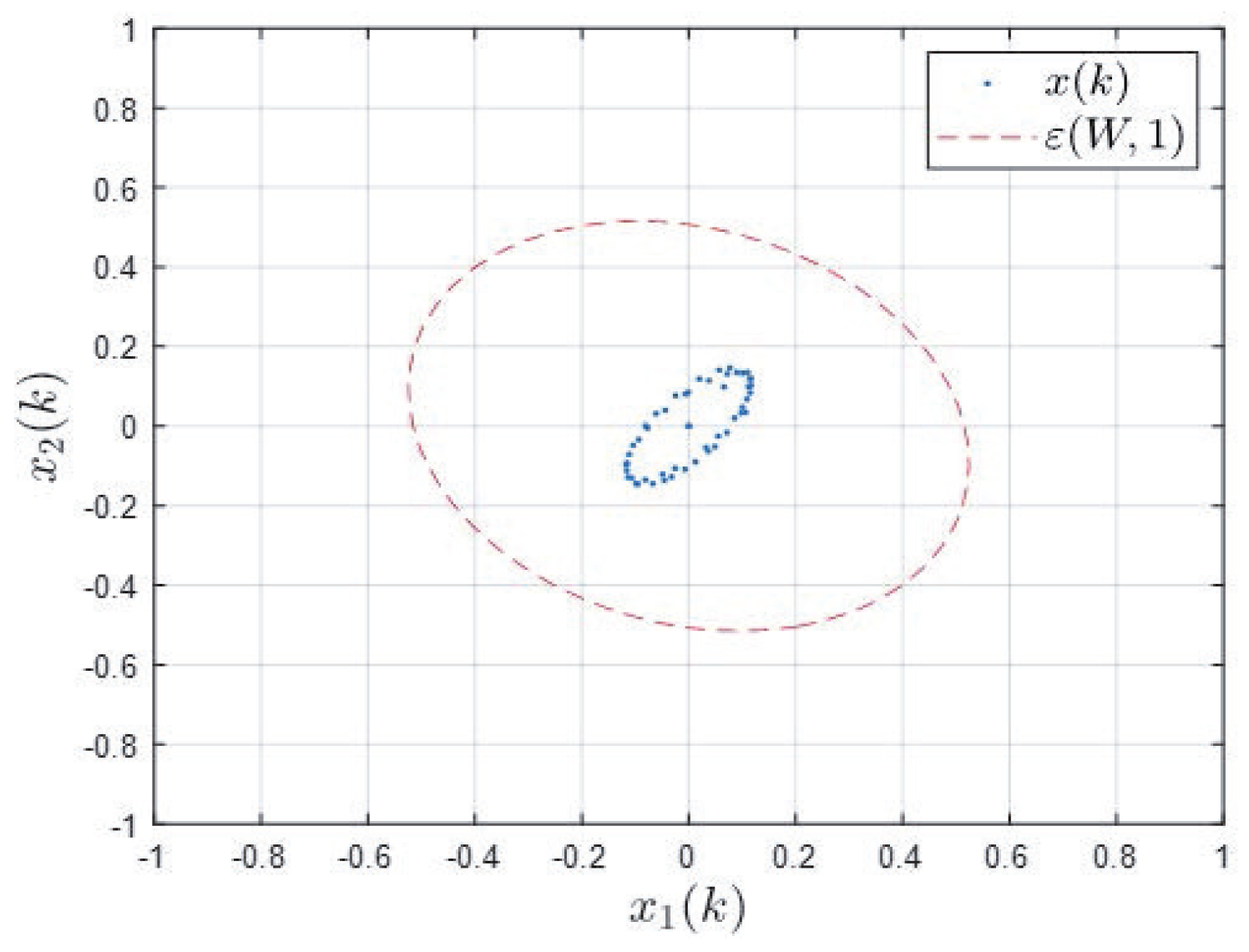
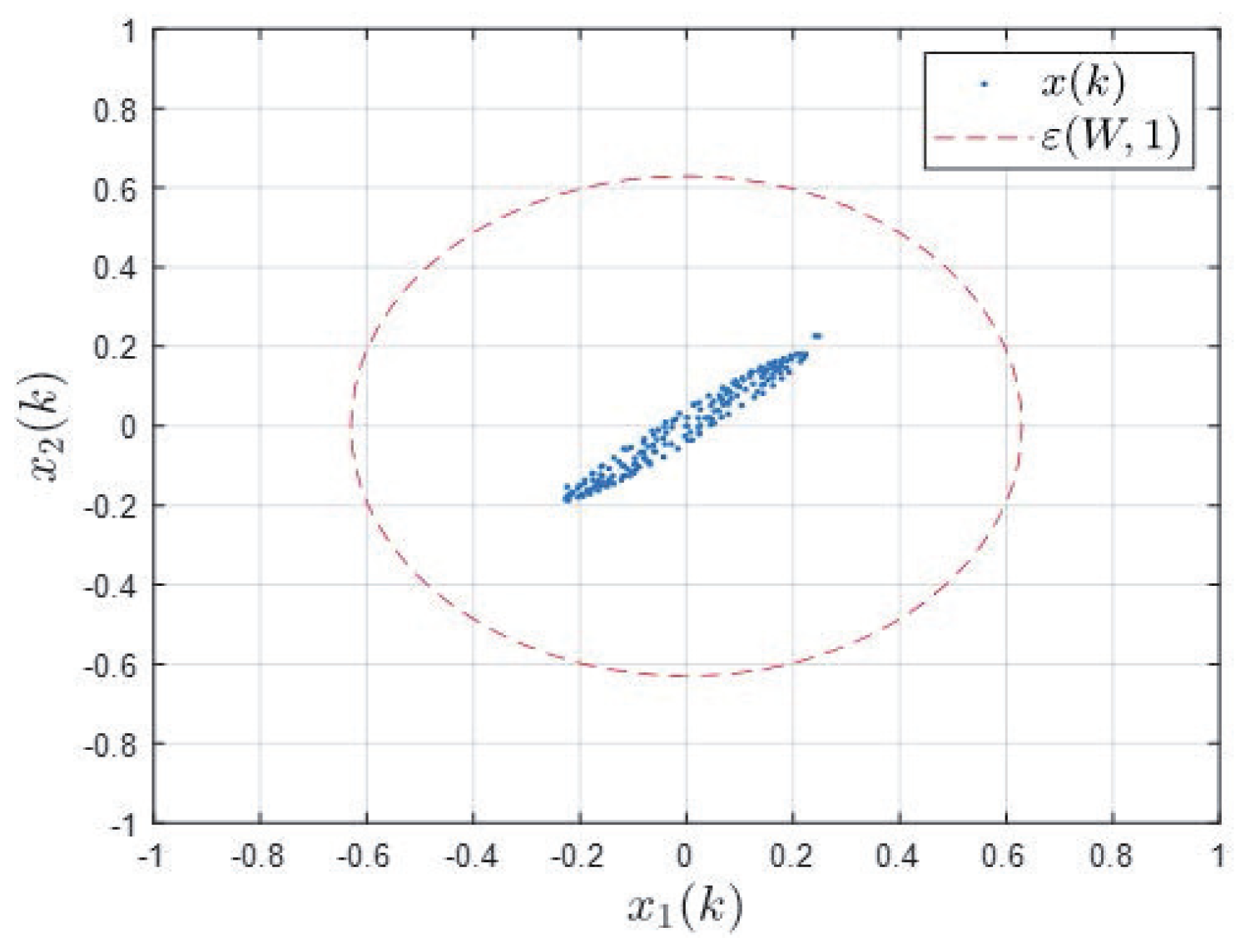
Example 1.

Consider a time-delay discrete generalized system with the following parameters: $E=\left[\begin{array}{cc}1& 0\hfill \\ 0& 0\hfill \end{array}\right],A=\left[\begin{array}{cc}0.8& -0.01\hfill \\ -0.5& 0.09\hfill \end{array}\right],A_h=\left[\begin{array}{cc}-0.02& 0\hfill \\ -0.1& -0.01\hfill \end{array}\right],B=\left[\begin{array}{c}0.2\\ 0.1\end{array}\right],{\omega }_m=0.1$. When $1\le h\left(k\right)\le 4$, take $h_1=1$, $h_2=4$ and $\beta =0.3$. From Theorem 1, we have $\gamma =1.7910$ and matrix $W=\left[\begin{array}{cc}3.7549& 0.6943\hfill \\ 0.6943& 3.8901\hfill \end{array}\right]$. The reachable sets of boundary ellipsoids and time-delay generalized systems are shown in Figure 1.

Example 2.

Consider a time-delay discrete generalized system with the following parameters: $E=\left[\begin{array}{cc}1& 0\hfill \\ 0& 0\hfill \end{array}\right],A=\left[\begin{array}{cc}0.8& 0.1\hfill \\ 0& 0.97\hfill \end{array}\right],A_h=\left[\begin{array}{cc}-0.1& 0\hfill \\ -0.1& -0.1\hfill \end{array}\right],B=\left[\begin{array}{c}0.1\\ 0.1\end{array}\right],{\omega }_m=0.1$. When $2\le h\left(k\right)\le 6$, $h_1=2$, $h_2=6$, and $\beta =0.5$, from Theorem 1, we have $\gamma =0.3969$ and matrix $W=\left[\begin{array}{cc}2.5195& -0.0001\hfill \\ -0.0001& 2.5193\hfill \end{array}\right]$. The reachable sets of the boundary ellipsoids and generalized systems are shown in Figure 2.

Examples 1 and 2 both illustrate the feasibility and accuracy of the method derived in this paper. The dotted ellipsoidal curve depicts the state trajectory of the singular system, while the dashed ellipsoidal curve represents the reachable set determined using the method presented in this paper. The experimental findings suggest that for a specified system, its state trajectory is contained within the reachable set of ellipses ascertained by employing the method proposed in this paper.

5. Conclusions

This article addresses the issue of estimating the reachable set for discrete-time generalized systems with time-varying delays and bounded peak inputs. In order to minimize the system’s conservatism, a novel condition for estimating the reachable set of time-varying time-delay discrete generalized systems has been derived using LMI. This is achieved through the application of an inverse convex combination and a discrete Wirtinger inequality as shown in [9]. Notably, the symmetric matrix featured in the obtained results does not necessitate positive definiteness. In comparison to decomposing the time-delay discrete generalized system under consideration into fast and slow subsystems, the proposed method is more straightforward and involves fewer variables. The efficacy and superiority of the achieved results have been validated through numerical examples. The method and conclusion in this paper can also be extended to the fractional discrete time generalized time-delay systems with perturbations [31].

References

- Osorio-Gordillo, G.L.; Darouach, M.; Astorga-Zaragoza, C.M.; Boutat-Baddas, L. Generalised dynamic observer design for Lipschitz non-linear descriptor systems. IET Control Theory Appl. 2019, 13, 2270–2280. [Google Scholar] [CrossRef]
- Li, J.; Feng, Z.; Zhang, C. Reachable Set Estimation for Discrete-Time Singular Systems. Asian J. Control 2017, 19, 1862–1870. [Google Scholar] [CrossRef]
- Monje, C.A.; Chen, Y.; Vinagre, B.M.; Xue, D.; Feliu, V. Fractional Order Systems and Control-Fundamentals and Applications, 1st ed.; Springer: London, UK, 2010. [Google Scholar]
- Dai, L. Singular Control Systems; Springer: Berlin/Heidelberg, Germany, 1989. [Google Scholar]
- Jiang, Y.; Yang, H.; Ivanov, I.G. Reachable Set Estimation and Controller Design for Linear Time-Delayed Control System with Disturbances. Mathematics 2024, 12, 176. [Google Scholar] [CrossRef]
- Lam, J.; Zhang, B. Reachable set estimation for discrete-time linear systems with time delays. Int. J. Robust Nonlinear Control 2015, 52, 146–153. [Google Scholar] [CrossRef]
- Nguyen, D. Reachable set bounding for linear-discrete-time systems with delays and bounded disturbances. J. Optim. Appl. 2013, 157, 96–107. [Google Scholar]
- Feng, Z.; Lam, J. On reachable set estimation of singular systems. Automatica 2015, 52, 146–153. [Google Scholar] [CrossRef]
- Xu, S.; Lam, J. Robust Control and Filtering of Singular Systems; Springer: Berlin/Heidelberg, Germany, 2006. [Google Scholar]
- Zuo, Z. Reachable set estimation for linear systems in the presence of both discrete and distributed delays. IET Control Theory Appl. 2011, 15, 1808–1812. [Google Scholar] [CrossRef]
- Kwon, O. On the reachable set bounding of uncertain dynamic systems with time-varying delays and disturbances. Inf. Sci. 2011, 181, 3735–3748. [Google Scholar] [CrossRef]
- Feng, Z.; Zheng, W.X.; Wu, L.G. Reachable set estimation of T-S fuzzy systems with time-varying delay. IEEE Trans. Fuzzy Syst. 2016, 25, 878–891. [Google Scholar] [CrossRef]
- Ma, X.; Zhang, Y.Y.; Huang, J. Reachable set estimation and synthesis for semi-Markov jump systems. Mathematics 2022, 609, 376–386. [Google Scholar] [CrossRef]
- Zhao, J. A new result on reachable set estimation for time-varying delay singular systems. Int. J. Robust Nonlinear Control 2020, 49, 3–11. [Google Scholar] [CrossRef]
- Huang, Y.; Tang, Q.; Yu, B. Partial Singular Value Assignment for Large-Scale Systems. Axioms 2023, 12, 1012. [Google Scholar] [CrossRef]
- Zhang, Z.H.; Feng, Z.G. Enclosing ellipsoid-based reachable set estimation for discrete-time singular systems. Int. J. Robust Nonlinear Control 2022, 32, 9294–9306. [Google Scholar] [CrossRef]
- Zhu, S.; Gao, Y.; Hou, Y.X.; Yang, C.Y. Reachable Set Estimation for Memristive Complex-Valued Neural Networks with Disturbances. IEEE Trans. Neural Networks Learn. Syst. 2023, 34, 11029–11034. [Google Scholar] [CrossRef] [PubMed]
- Zhang, Z.H.; Wang, X.S.; Xie, W.B.; Shen, Y. Reachable set estimation for uncertain nonlinear systems with time delay. Optim. Control Appl. Methods 2020, 41, 1644–1656. [Google Scholar] [CrossRef]
- Zhang, Z.H.; Wang, Z.H.; Wang, Y.; Shen, Y.; Liu, Y.P. Zonotopic reachable set estimation for bilinear systems with time-varying delays. Int. J. Syst. Sci. 2020, 52, 848–856. [Google Scholar] [CrossRef]
- Chen, R.H.; Guo, M.X.; Zhu, S.; Qi, Y.Q.; Wang, M.; Hu, J.H. Reachable set bounding for linear systems with mixed delays and state constraints. Appl. Math. Comput. 2022, 425, 127085. [Google Scholar] [CrossRef]
- Ivanov, I. The LMI Approach for Stabilizing of Linear Stochastic Systems. Int. J. Stoch. Anal. 2013, 2013, 281473. [Google Scholar] [CrossRef]
- Yang, H.; Si, X.; Ivanov, I.G. Constrained State Regulation Problem of Descriptor Fractional-Order Linear Continuous-Time Systems. Fractal Fract. 2024, 8, 255. [Google Scholar] [CrossRef]
- Yang, H.; Zhou, M.; Pan, P.; Zhao, M. Nonnegativity, stability analysis of linear discrete-time positive descriptor systems: An optimization approach. Bull. Pol. Acad. Sci. Tech. Sci. 2018, 66, 1–7. [Google Scholar]
- Song, Q.; Liang, J.; Wang, Z. Passivity analysis of discrete-time stochastic neural networks with time-varying delays. Neurocomputing 2009, 72, 1782–1788. [Google Scholar] [CrossRef]
- Park, P.; Jeong, W.K.; Jeong, C. Reciprocally convex approach to stability of systems with time-varying delays. Automatica 2011, 47, 235–238. [Google Scholar] [CrossRef]
- Zhao, J.; Hu, Z. Improved Results on Reachable Set Estimation of Linear Systems. Int. J. Control Autom. Syst. 2019, 17, 1141–1148. [Google Scholar] [CrossRef]
- Bower, S.; Taheri, E. Rapid Approximation of Low-Thrust Spacecraft Reachable Sets within Complex Two-Body and Cislunar Dynamics. Mathematics 2024, 11, 380. [Google Scholar]
- Li, T.C.; Zheng, C.X.; Feng, Z.G.; Dinh, T.N.; Raïssi, T. Real-time reachable set estimation for linear time-delay systems based on zonotopes. Int. J. Syst. Sci. 2023, 54, 1639–1647. [Google Scholar] [CrossRef]
- Nam, T.; Pathirana, N.; Trinh, H. Discrete Wirtinger-based inequality and its application. J. Frankl. Inst. 2015, 352, 1893–1905. [Google Scholar] [CrossRef]
- Seuret, A.; Gouaisbaut, F. Wirtinger-based integral inequality: Application to time-delay systems. Automatica 2013, 49, 2860–2866. [Google Scholar] [CrossRef]
- Zhang, T.; Li, Y. Global exponential stability of discrete-time almost automorphic Caputo–Fabrizio BAM fuzzy neural networks via exponential Euler technique. Knowl.-Based Syst. 2022, 246, 108675. [Google Scholar] [CrossRef]