Deep Q-Networks for Minimizing Total Tardiness on a Single Machine ^†

Abstract

This paper considers the single-machine scheduling problem of total tardiness minimization. Due to its computational intractability, exact approaches such as dynamic programming algorithms and branch-and-bound algorithms struggle to produce optimal solutions for large-scale instances in a reasonable time. The advent of Deep Q-Networks (DQNs) within the reinforcement learning paradigm could be a viable approach to transcending these limitations, offering a robust and adaptive approach. This study introduces a novel approach utilizing DQNs to model the complexities of job scheduling for minimizing tardiness through an informed selection utilizing look-ahead mechanisms of actions within a defined state space. The framework incorporates seven distinct reward-shaping strategies, among which the Minimum Estimated Future Tardiness strategy notably enhances the DQN model’s performance. Specifically, it achieves an average improvement of 14.33% over Earliest Due Date (EDD), 11.90% over Shortest Processing Time (SPT), 17.65% over Least Slack First (LSF), and 8.86% over Apparent Tardiness Cost (ATC). Conversely, the Number of Delayed Jobs strategy secures an average improvement of 11.56% over EDD, 9.10% over SPT, 15.01% over LSF, and 5.99% over ATC, all while requiring minimal computational resources. The results of a computational study demonstrate DQN’s impressive performance compared to traditional heuristics. This underscores the capacity of advanced machine learning techniques to improve industrial scheduling processes, potentially leading to decent operational efficiency.

1. Introduction

Scheduling refers to allocating various limited resources such as materials, machines, technicians, vehicles, etc. to concerned economic activities over the time horizon, subject to technical constraints, so as to optimize certain managerial criteria. The makespan, the total completion time, the number of late jobs, and the total tardiness are among the widely used performance measures in industry and academia. Scheduling problems constitute a prominent research area in management science and operations research due to the theoretical interest and challenges as well as a wide spectrum practical applications in manufacturing, logistics, service, and project management, just to name a few. Along with the booming trend of artificial intelligence, machine learning techniques are widely adopted to tackle hard scheduling problems [1]. In this paper, we use the total tardiness minimization problem as an example to illustrate the use of problem-specific optimization heuristic information to enrich the performance of a machine learning approach. Tardiness is the late deviation of order fulfillment beyond the due date quoted to its client. Total tardiness, one of the classical managerial criteria investigated in scheduling researches, is concerned about operational efficiency, customer satisfaction or service quality, and overall system performance. Consider the example instance of five jobs or production orders shown in

Table 1. Processing times and due dates of jobs.

Jobs	Processing Times	Due Dates
1	2	6
2	3	8
3	4	9
4	2	7
5	5	11

. Each job is characterized by a required production length and a due date quoted to its customer.

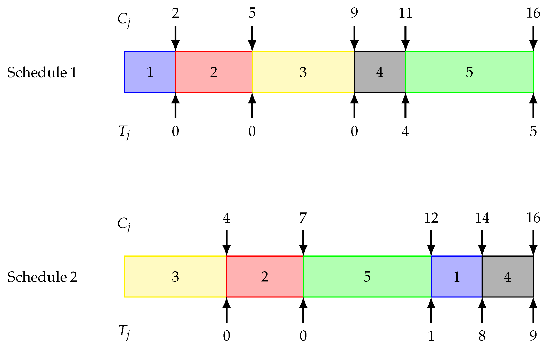
Consider the two distinct schedules shown in Figure 1 for processing the five jobs:

• Schedule 1: 1 → 2 → 3 → 4 → 5 and Schedule 2: 3 → 2 → 5 → 1 → 4. In schedule 1, job 4 has a tardiness of $11-7=4$ units, and job 5 has a tardiness of $16-11=5$ units. The total tardiness is 9.
• Schedule 2: The tardiness of job 5 is $12-11=1$ unit, $14-6=8$ units for job 1, and $16-7=9$ units for job 4. The total tardiness is 18.

Figure 1. Example schedules and their job tardiness values.

Figure 1. Example schedules and their job tardiness values.

The example demonstrates that different processing sequences may yield objective values (total tardiness) that are significantly deviate from one another. The studied problem is to determine a schedule that attains the minimum tardiness penalty.

We formally define the studied problem as follows. The processing environment has a single machine and the given is a set of n jobs $\mathcal{J}=\{1,2,\dots ,n\}$, in which job i is associated with a processing time $p_i$ and a due date $d_i$. In a particular schedule, the completion time of job i is denoted by $C_i$. The tardiness of job i is defined as $T_i=max\{0,C_i-d_i\}$, reflecting job i’s late completion deviated from its due date. If it is completed by the due date, the tardiness is zero. The objective is to determine a schedule whose total tardiness ${\sum }_{i=1}^n{T}_i$ is a minimum. In Ref. [2], the three-field notation $\alpha \left|\beta \right|\gamma$ is introduced as a canonical scheme to denote scheduling problems. The field $\alpha$ indicates the machine environment, e.g., a single machine, parallel machines, or flow shops; the second field $\beta$ introduce job characteristics or restrictions, e.g., release dates, due dates, or setup times; and the last field $\gamma$ prescribes the objective to optimize, e.g., the makespan, the number of late jobs, or the total tardiness. The studied problem is described as $1\left|\right|{\sum }_i{T}_i$, where 1 indicates that a single machine is available for processing, and the third field ${\sum }_i{T}_i$ prescribes the objective function of total tardiness. The second field is empty as due date constraints are implicit in the objective function. The problem setting of $1\left|\right|{\sum }_i{T}_i$ follows three assumptions commonly adopted in the literature: (1) The machine can process at most one job at any time. (2) No preemption or interruptions of jobs is allowed, i.e., once a job starts, it occupies the machine until its completion. (3) All cited variables and parameters have non-negative integer values.

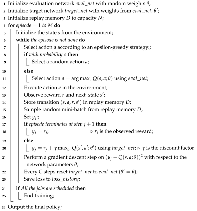
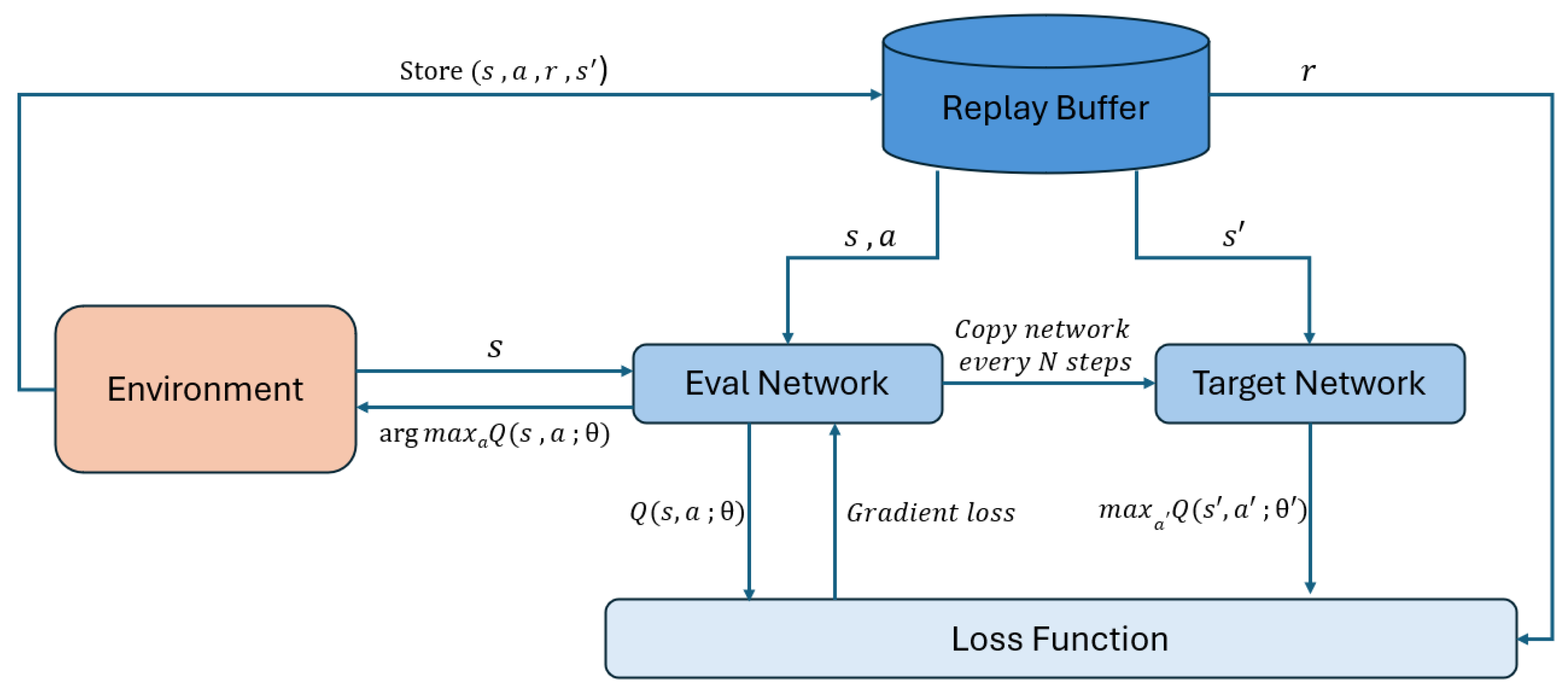
The total tardiness minimization problem $1\left|\right|{\sum }_i{T}_i$ is shown to be NP-hard by Du and Leung [3]. It is, therefore, very unlikely that algorithms that can produce optimal solutions in a reasonable time can be designed. Beyond the optimization methods, machine learning techniques, due to their successful applications in for example [1,4,5,6], also provide another solution-finding approaches. This paper explores the application of Deep Q-Networks (DQNs) to the static single-machine total tardiness problem, advancing beyond traditional Q-learning techniques typically used in dynamic scheduling contexts. Our research uniquely addresses static scheduling where jobs and their respective processing times and due dates are predefined prior to the training phase, contrasting with prior studies that simulate job arrivals through Poisson distributions during the training interval. This methodological shift allows for a precise evaluation of DQNs’ capabilities in a controlled environment.

The core objective of this study is to rigorously compare different reward mechanisms within the DQN framework to optimize decision-making outcomes for scheduling problems. We differentiate between local rewards, which focus on the immediate consequences of job selections, and global rewards, which consider the long-term impact of decisions on the sequence of job completions. Our experimental setup involves a detailed investigation into mixed rewards, combining local and global incentives, versus exclusive use of global rewards. Additionally, we explore various methodologies for calculating global rewards, aiming to pinpoint the most effective approach for leveraging DQNs in reducing total tardiness. Through this comparative analysis, our research seeks to identify and validate the most robust method for deploying deep reinforcement learning in the context of static scheduling, ultimately enhancing the precision and reliability of scheduling decisions.

The rest of this paper is organized as follows. Section 2 reviews related work in the literature on scheduling problems on total tardiness minimization and DQNs. The framework and the detailed design of constituents of our DQN are presented in Section 3. To evaluate the performance of the proposed approach, we conducted computational experiments. Section 4 includes the experiment design and the data generation scheme adopted in the computational study. The resultant computational statistics and elaborative analysis are given in Section 5. We summarize this study and suggest future research directions in Section 6.

2. Literature Review

Within the domain of single-machine total tardiness problems, a diversity of algorithmic approaches vies to address the inherent complexity. Exact algorithms, particularly dynamic programming and branch-and-bound methods, aspire to unravel the problem with unwavering accuracy, offering solutions of optimal caliber at the cost of computational intensity. Conversely, heuristic algorithms eschew the rigor of accuracy in favor of expediency, delivering robust solutions with commendable efficiency. Recently, the spotlight has shifted towards reinforcement learning (RL), an adaptive approach that progressively refines its decision-making process through continuous interaction with the problem space. Distinct from deterministic algorithms, RL’s iterative learning paradigm embodies a dynamic evolution of strategy, emphasizing resilience and adaptability. This burgeoning field holds promise for significant advancements in production scheduling, proposing a paradigm where algorithms are not merely solutions but entities capable of growth and self-improvement within their operational environments.

Dynamic programming (DP) and branch-and-bound (B&B) algorithms have been at the forefront of solving the single-machine total tardiness problem optimally. In Table 2, we provide a consolidated overview of the diverse algorithms that have been proposed in the literature for tackling the single-machine total tardiness problem. Srinivasan [7] developed a hybrid algorithm using DP that implements Emmons’ dominance conditions [8], providing a fundamental understanding of job precedence relationships. Baker [9] contributed to this approach with a chain DP algorithm that also utilizes these conditions for enhanced efficiency. Lawler [10] furthered this line of work with a pseudo-polynomial algorithm tailored for the weighted tardiness problem, yielding a significant reduction in the worst-case running time to $O\left(n^{4}P\right)$ or $O\left(n^5{p}_{\max }\right)$, with P and $p_{\max }$ representing the sum and maximum of processing times, respectively. To improve upon these methodologies, Potts and Van Wassenhove [11] recommended augmentations to Lawler’s decomposition DP algorithm, integrating it with their refined decomposition theorem for more nuanced scheduling solutions.

In parallel with DP, B&B strategies have also shown immense promise. Pioneering works by Elmaghraby [12] and Shwimer [13] introduced B&B algorithms that efficiently handle the intricacies of the total tardiness problem. The efforts by Rinnooy Kan et al. [14] refined lower bound calculations for a broad cost function via a linear assignment relaxation, enhancing the precision of B&B techniques. Fisher [15] utilized a dual problem approach grounded in Lagrangian relaxation to devise an algorithm with profound implications for computational speed and solution quality. Picard and Queyranne [16] merged the complexities of the traveling salesman problem within a multipartite network into the B&B framework, leading to significant improvements in minimizing tardiness in single-machine scheduling scenarios. To cap these developments, Sen et al. [17] exploited Emmons’ conditions to lay down job precedence relationships, paving the way for an implicit enumeration scheme that remarkably requires only $O\left(n^2\right)$ memory space, thereby combining the rigor of B&B algorithms with the practicality needed for real-world scheduling.

The study of heuristic algorithms for the single-machine total tardiness problem presents a diverse landscape of strategies, each with its unique approach to minimizing tardiness under varying constraints. Baker et al. [18] explore priority rules for minimizing tardiness, emphasizing a “modified due-date rule” (MDD) that adapts efficiently to varying due-date constraints, where $\mathrm{MDD}=max(C+p_i,d_i)$. C is the current completion time, $p_i$ is the processing time of job i, and $d_i$ is the due date of job i. Carroll and Donald [19] introduced the COVERT rule with a computational complexity of $O\left(n^2\right)$, targeting job shop sequencing by prioritizing jobs based on the descending order of their cost/processing time ratio. Applied to the $1\left|\right|{\sum }_i{T}_i$ problem, this rule selects the next job by estimating the likelihood of job i being tardy if not scheduled immediately, effectively calculating a priority index for sequencing decisions. Morton et al. 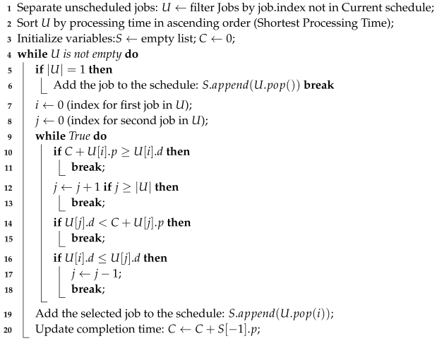[20] proposed the Apparent Urgency (AU) heuristic for scheduling jobs at the decision time t by prioritizing jobs using $A{U}_i={\displaystyle \frac{1}{p_i}}exp\left\{-max\left[0,d_i-t-p_i\right]\right\}/(k\times \overline{p})$, with k adjusting for due date tightness and $\overline{p}$ as the average processing time, facilitating prioritization amidst potential job conflicts. Panwalkar et al. [21] introduced the PSK heuristic, a construction method ordering jobs by the Shortest Processing Time (SPT). The PSK heuristic iterates through n passes, selecting and scheduling an “active” job each time. The selection process, moving left to right through unscheduled jobs, determines an active job as one that would be tardy if scheduled next. An active job i remains so unless a job j to its right with $d_j<d_i$ is found, implying job j becomes the new active job. This process continues until a tardy-active job is found or the last unscheduled job is activated and scheduled. The PSK heuristic operates with a complexity of $O(n^{2}logn)$.

Table 2. Summary of exact algorithms for single-machine total tardiness problem.

Reference	Main Results
Dynamic Programming (DP)
Srinivasan [7]	Hybrid algorithm incorporating Emmons’ dominance conditions.
Baker [9]	Chain DP algorithm utilizing Emmons’ conditions for efficiency.
Lawler [10]	Pseudo-polynomial algorithm for weighted tardiness with improved running time.
Potts and Van Wassenhove [11]	Enhancements to DP algorithm, including application of a revised decomposition theorem.
Branch-and-Bound (B&B)
Elmaghraby [12]	Early B&B algorithm for single-machine total tardiness scheduling.
Shwimer [13]	B&B algorithm tailored for the single-machine total tardiness problem.
Rinnooy Kan et al. [14]	Precise lower bounds via linear assignment relaxation.
Fisher [15]	Algorithm using a dual problem approach based on Lagrangian relaxation.
Picard and Queyrann [16]	Method integrating aspects of travelling salesman problem in B&B enumeration.
Sen et al. [17]	Implicit enumeration scheme based on job precedence relationships requiring $O\left(n^2\right)$ storage.
Naidu [22]	Four decomposition conditions that can help the search process for finding exact solutions.

Table 2. Summary of exact algorithms for single-machine total tardiness problem.

Reference	Main Results
Dynamic Programming (DP)
Srinivasan [7]	Hybrid algorithm incorporating Emmons’ dominance conditions.
Baker [9]	Chain DP algorithm utilizing Emmons’ conditions for efficiency.
Lawler [10]	Pseudo-polynomial algorithm for weighted tardiness with improved running time.
Potts and Van Wassenhove [11]	Enhancements to DP algorithm, including application of a revised decomposition theorem.
Branch-and-Bound (B&B)
Elmaghraby [12]	Early B&B algorithm for single-machine total tardiness scheduling.
Shwimer [13]	B&B algorithm tailored for the single-machine total tardiness problem.
Rinnooy Kan et al. [14]	Precise lower bounds via linear assignment relaxation.
Fisher [15]	Algorithm using a dual problem approach based on Lagrangian relaxation.
Picard and Queyrann [16]	Method integrating aspects of travelling salesman problem in B&B enumeration.
Sen et al. [17]	Implicit enumeration scheme based on job precedence relationships requiring $O\left(n^2\right)$ storage.
Naidu [22]	Four decomposition conditions that can help the search process for finding exact solutions.

A local search heuristic is an improvement method based on successive iterations of neighborhood construction and elite neighbor selection. Given an incumbent solution, the best one among its neighbor solutions is selected as the solution of the next iteration. The neighborhood can be defined in various ways. The procedure iterates until no more improvement is possible. For minimizing the total tardiness, local search heuristics, like those proposed by Fry et al. [23], introduce an improvement method based on adjacent pairwise interchange (API) to reduce mean tardiness in single-machine scheduling. The effectiveness of the API heuristic remains consistent across various problem sizes and due date constraints. Holsenback and Russell [24] present a heuristic leveraging Net Benefit of Relocation (NBR) to identify the optimal last job in a sequence, aiming to minimize total tardiness. Starting with an EDD schedule, the heuristic applies a dominance rule, inspired by Emmons’ conditions, and the NBR analysis to relocate jobs for improved tardiness outcomes. This process iterates until no further beneficial relocations are detected, with the algorithm exhibiting a complexity of $O\left(n^2\right)$. Wilkerson and Irwin [25] introduced the WI heuristic, a hybrid approach combining construction and local search techniques through adjacent job pairwise interchanges. The heuristic evaluates schedule efficiency using the loss function $max(0,C_i-D_i)$, where $C_i$ is the completion time of job i and $D_i$ its due date; while generally not guaranteeing optimality, conditions for achieving optimal schedules are specified. A key principle of the WI heuristic is prioritizing jobs with nearer due dates, except under certain conditions where shorter jobs precede, using this criterion to systematically build a job sequence. Ho and Chang [26] introduce a hybrid heuristic incorporating construction and local search, defined by the Traffic Congestion Ratio (TCR) for single-machine scheduling ($1\left|\right|\sum T_i$) and potentially multi-machine ($P\left|\right|\sum T_i$) contexts. TCR is calculated as $TCR={\displaystyle \frac{\overline{p}\times n}{\overline{d}\times m}}$, where $\overline{p}$ and $\overline{d}$ represent the average processing time and due date across n jobs, respectively, and m is the number of machines. They employ TCR to assess shop congestion and generate a priority index $R_i$ for each job i,

$$R_i=w_d\times {\displaystyle \frac{d_i}{max{d}_j}}+(1-w_d)\times {\displaystyle \frac{p_i}{max{p}_j}},$$

with $w_d$ adjusted based on TCR and a constant K. Jobs are initially sequenced by increasing $R_i$ values, followed by improvements through adjacent pairwise interchanges.

Finally, the decomposition heuristics by Potts and Van Wassenhove [27] optimize the sequence placement of the longest job j through a set of guiding inequalities. These inequalities ensure a strategic fit for job j at a position k, considering the cumulative processing times of preceding jobs and the due times of subsequent jobs, maintaining job j’s precedence in the face of adjacent job comparisons, and securing job j as the last in the sequence when due. This systematic use of inequalities within the DEC/WI/D heuristic effectively drives down total tardiness, with the heuristic proving robust across scenarios and showcasing a computational complexity of $O\left(n^2\right)$, even when position k selections are randomized. The comprehensive results captured in

Table 3. Summary of heuristic approaches for single-machine total tardiness problem.

Heuristic	Reference	#Opt (Out of 125)	Average CPU Time (s)
Construction and Local Search Heuristics
API	Fry et al. [23]	76	4.12
NBR	Holsenback and Russell [24]	27	0.97
WI	Wilkerson and Irwin [25]	55	0.39
PSK	Panwalkar et al. [21]	87	0.01
Decomposition Heuristics
DEC/WI/D	Potts and Van Wassenhove [27]	98	2.92
DEC/PSK/D	Potts and Van Wassenhove [27]	99	2.44

underscore the effectiveness of heuristic strategies in solving the single-machine total tardiness problem. These results, computed by Koulamas and Christos [28] for construction heuristics and local search methods, and by Potts and Van Wassenhove [27] for decomposition heuristics, offer insightful benchmarks for the performance of each approach.

Recent advancements in machine learning, particularly reinforcement learning (RL), have significantly impacted addressing complex scheduling challenges, demonstrating considerable promise. RL’s adaptability and intelligent decision-making in dynamic environments position it as a powerful tool for optimizing scheduling processes.

Table 4. Summary of reinforcement learning applications in single-machine scheduling.

Reference	Main Contributions
Wang and Usher [29]	Employed Q-learning to optimize dispatch rule selection for reducing mean tardiness, using a policy table based on job queue statuses.
Kong and Wu [30]	Targeted multiple objectives through RL, with state representations based on job slack, using different dispatching rules.
Idrees et al. [31]	Investigated a dual-objective problem involving tardiness reduction and extra labor costs, employing lambda-SMART algorithm for policy optimization.
Xanthopoulos et al. [32]	Proposed dynamic scheduling approaches using RL and Fuzzy Logic to address uncertainties, aiming to minimize earliness and tardiness.
Li et al. [33]	Explored the effectiveness of various RL algorithms, including Q-learning and Sarsa, on the online scheduling problem to reduce total tardiness.
Bouška et al. [34]	Designed a deep neural network as an estimator of the objective value based on Lawler’s decomposition and the symmetric decomposition proposed of Della Croce et al. [35].
Hassan et al. [1]; Kayhan and Yildiz [36]	Presented comprehensive reviews of using machine learning techniques in machine scheduling problems

presents a concise summary of significant research efforts employing reinforcement learning in single-machine scheduling. The pioneering work of Wang and Usher [29] in applying Q-learning to single-machine scheduling aimed at minimizing mean tardiness showcases the efficacy of a state–action value table to navigate through various dispatching rules—Earliest Due Date (EDD), Shortest Processing Time (SPT), and First In First Out (FIFO)—based on the job queue’s status. Their study not only validates Q-learning’s potential in policy refinement but also elucidates significant factors affecting RL’s effectiveness in production scheduling environments.

Building on this foundation, Kong and Wu [30] extended RL applications to meet three distinct scheduling objectives, employing unique state representations like average slack and maximum slack of jobs in the buffer. This approach demonstrates RL’s flexibility in optimizing scheduling goals through appropriate dispatch rule selection. Similarly, Idrees et al. [31] navigated a dual-objective scheduling dilemma, juxtaposing job tardiness minimization with the cost implications of additional labor. Their strategic use of queue length as a state space and exploring multiple action strategies emphasizes RL’s nuanced decision-making prowess, underscored by the lambda-SMART algorithm for online policy optimization.

Xanthopoulos et al. [32] ventured into dynamic scheduling realms under uncertainty, combining RL with Fuzzy Logic and multi-objective evolutionary optimization. Their approach, aimed at minimizing earliness and tardiness, leverages a state representation embodying the total workload and mean slack, underscoring the adaptability of RL to dynamic scheduling environments. Further, Li et al. [33] evaluated the performance of various RL algorithms, including Q-learning, Sarsa, Watkins’s Q($\lambda$), and Sarsa($\lambda$), in online single-machine scheduling. Their focus on dynamically selecting the next job from the queue for processing illustrates the comprehensive potential of RL in reducing total tardiness and enhancing scheduling performance. Bouška et al. [34] designed a deep neural network for estimating the objective value using Lawler’s decomposition and the symmetric decomposition of Della Croce et al. [35]. They also presented a novel method for generating instances. The optimality gaps yielded by their model is only 0.26% for a large job set of 800 jobs. for a more comprehensive review on ML applications in machine scheduling, the reader is referred to [1,36].

Despite these contributions, the exploration of RL in single-machine scheduling remains relatively untapped, presenting a rich area for further investigation. Our research builds upon this limited but foundational work, offering new avenues to delve deeper into the potential of RL in optimizing single-machine scheduling tasks. By exploring innovative state representations, action strategies, and algorithmic improvements, our research advances the application of reinforcement learning in the single-machine total tardiness problem by employing Deep Q-Networks (DQNs), diverging from the conventional Q-learning approaches prevalent in the existing literature. Focusing on a specific set of states and actions, our aim is to enhance operational efficiency and introduce innovative perspectives on the use of RL in scheduling tasks.

3. Design of DQN Framework

3.1. Deep Q Network

Consider a Markov decision process defined by the tuple $(X,A,P,R)$, where X is the set of all possible states, A represents the set of all possible actions, P is the probability function of state transition, and R is the reward function. In this framework, a computational agent operates within a discrete finite environment. The agent interacts with the environment over a series of discrete time steps, indexed by t. At each time step t, the agent observes the current state $x_t\in X$ and chooses an action $a_t\in A$. This setup forms a controlled Markov process, where the agent’s actions influence the state transitions and consequent rewards. Upon selecting an action, the agent receives a probabilistic reward $r_t$ with a mean value ${\mathcal{R}}_{x_t}\left(a_t\right)$, and the environment transitions to a new state $x_{t+1}$ according to the probabilistic function P, described mathematically as:

$$\mathrm{Prob}[x_{t+1}=y\mid x_t,a_t]=P_{x_t,y}\left[a_t\right]$$

(1)

The agent aims to find an optimal policy that maximizes the total discounted expected reward. This objective is represented by the value of state x under policy $\pi$. The value function $V^{\pi }\left(x\right)$ is defined as the sum of the immediate reward received when the agent takes action $\pi \left(x\right)$ in state x, and the expected future rewards from state x after taking action $\pi \left(x\right)$. Mathematically, this is expressed as:

$$V^{\pi }\left(x\right)={\mathcal{R}}_x\left(\pi \left(x\right)\right)+\gamma \sum _y{P}_{xy}\left[\pi \left(x\right)\right]V^{\pi }\left(y\right)$$

(2)

Here, ${\mathcal{R}}_x\left(\pi \left(x\right)\right)$ is the immediate reward, $\gamma$ is the discount factor, $P_{xy}\left[\pi \left(x\right)\right]$ is the probability of transitioning from state x to state y under action $\pi \left(x\right)$, and $V^{\pi }\left(y\right)$ is the value of the next state y under policy $\pi$. Bellman and Dreyfus [37] ensure that an optimal stationary policy ${\pi }^{\ast }$ exists, such that:

$$V^{{\pi }^{\ast }}\left(x\right)=V^{\ast }\left(x\right)=\underset{a}{max}\left\{{\mathcal{R}}_x\left(a\right)+\gamma \sum _y{P}_{xy}\left[a\right]V^{\ast }\left(y\right)\right\}$$

(3)

To determine the optimal policy, Watkins [38] introduces Q-learning as an incremental dynamic programming technique. In this context, the Q-value is defined as the expected discounted reward when following policy $\pi$ after taking action a in state x:

$$Q^{\pi }(x,a)={\mathcal{R}}_x\left(a\right)+\gamma \sum _y{P}_{xy}\left[a\right]V^{\pi }\left(y\right)$$

(4)

The goal of Q-learning is to estimate the Q-value associated with the optimal policy, specifically by identifying ${max}_{a}Q(x,a)$. To accomplish this, Q-learning iteratively refines its estimates of the Q-values. This iterative estimation process can be represented by the following update rule:

$$Q(s,a)\leftarrow Q(s,a)+\alpha \left(r+\gamma \underset{a^{\prime }}{max}Q(s^{\prime },a^{\prime })-Q(s,a)\right)$$

(5)

where $\alpha$ denotes the learning rate, r is the reward received upon taking action a in state s, $s^{\prime }$ represents the subsequent state, and $a^{\prime }$ signifies the next action to be evaluated. The Q-learning algorithm updates the Q-values based on the temporal difference error, which measures the difference between the current Q-value and the learned estimate. By iteratively applying this update rule, Q-learning converges to the optimal Q-values, thereby enabling the determination of the optimal policy that maximizes the total discounted expected reward over time.

Deep Q-Networks (DQNs) build upon traditional Q-learning by integrating deep neural networks to estimate the Q-function, which is particularly advantageous in environments with high-dimensional state spaces. The architecture of a DQN consists of several crucial components: an experience replay buffer, a target network, and an epsilon-greedy strategy for action selection. The experience replay buffer accumulates transitions at each timestep in the form of tuples $(s,a,r,s^{\prime })$, thereby decoupling consecutive experiences and allowing the network to learn from a diverse set of past experiences. This method helps to diminish the correlation between observations and smooths out fluctuations in the data distribution.

The target network, which shares the same architecture as the primary network but with periodically updated weights, contributes significantly to the stability of the learning process. It generates the Q-value predictions used as stable targets during the learning updates for the primary network. The epsilon-greedy strategy is crucial for balancing exploration and exploitation, ensuring that the agent explores the environment sufficiently while exploiting its growing knowledge base.

In our reinforcement learning setup, we use a neural network to approximate the Q-values for the state–action pairs. This network is designed with several layers to increase its representational capacity. The architecture begins with an input layer that takes the flattened state matrix as input, followed by a series of fully connected layers. Specifically, the first layer maps the input states to a hidden layer, which is then followed by a second layer that doubles the number of neurons. A third fully connected layer maintains the same number of neurons as the second layer. To prevent overfitting, a dropout layer with a dropout probability of 0.2 is applied after the third layer. The fourth layer reduces the number of neurons back to the original size of the hidden layer. Finally, the output layer produces the Q-values for each possible action. Each layer uses the Leaky ReLU activation function with a negative slope of 0.01 to introduce non-linearity into the model and help it learn complex patterns. Figure 2 illustrates the architecture of the neural network.

The training process of a DQN agent involves several sequential and iterative steps, as visualized in Figure 3. Initially, the agent observes the state s and selects an action a based on the epsilon-greedy policy derived from the current Q-values predicted by the evaluation network. After action execution, the environment transitions to a new state $s^{\prime }$, and the agent observes a reward r. This transition $(s,a,r,s^{\prime })$ is stored in the replay buffer.

Periodically, a batch of transitions is sampled from the buffer, and the evaluation network computes the current Q-values, $Q(s,a;\theta )$, while the target network estimates the future Q-values, ${max}_{a^{\prime }}Q(s^{\prime },a^{\prime };{\theta }^{-})$. The primary network’s weights are updated by minimizing the loss between these Q-values, typically using mean-squared error. Every N steps, the weights from the evaluation network are copied to the target network, which helps maintain the stability of the target values used in the training updates.

The training process involves iteratively updating the policy by sampling mini-batches from the experience replay buffer. We train our network using a mean squared error loss function between the predicted Q-values and the target Q-values, which are periodically updated from the evaluation network to the target network. We explore the impact of other enhancements such as prioritized experience replay, which weights the replayed experiences based on their temporal difference error, biasing the learning process towards more significant transitions. The convergence of the training process is monitored through episodic rewards and the evolution of loss over time. Algorithm 1 demonstrates the process involved in training a DQN agent for the total tardiness problem.

Algorithm 1: DQN Training for Total Tardiness Problem

3.2. State

For our DQN model, the state is represented by a matrix capturing the salient features of the scheduling environment, such as processing times, urgency, and job statuses. The action space is discrete, with each action corresponding to the selection of a job from the queue based on four heuristics. The reward function is defined to reflect the immediate impact of an action on total tardiness, penalizing tardiness, and rewarding actions that contribute to on-time job completion.The state space for the DQN model is represented by a matrix $\mathbf{M}$ of dimensions $2\times n$, where n is the total number of jobs. See Figure 4 for an illustration. Each row of this matrix provides the specific information as follows:

• Job Scheduling Status: The first row, ${\mathbf{M}}_{1,\times }$, is a binary vector indicating the scheduling status of each job. If job i is scheduled, the corresponding entry $M_{1,i}=1$; otherwise, $M_{1,i}=0$.
• Job Urgency: The second row, ${\mathbf{M}}_{2,\times }$, denotes the urgency of each job, calculated as the ratio of the remaining time until the job’s due date over its processing time. For job i, this is given by $M_{2,i}={\displaystyle \frac{d_i-t}{p_i}}$, where $d_i$ is the due date of job i, t is the current time, and $p_i$ is the processing time of job i.

Figure 4. Diagram of the state matrix.

Figure 4. Diagram of the state matrix.

3.3. Action

The discrete action space is comprised of actions where each action a corresponds to selecting a job based on one of four heuristic rules, which are as follows:

• Action 1 (EDD): Select the job that has the earliest due date. Formally, choose job i for which the due date $d_i$ is minimal among all unscheduled jobs.
• Action 2 (SPT): Select the job that has the shortest processing time. Formally, choose job i for which the processing time $p_i$ is minimal among all unscheduled jobs.
• Action 3 (LSF): Select the job that has the least slack. Slack for job i is defined as $d_i-(t+p_i)$, where t is the current time. The job with the minimal slack among all unscheduled jobs is chosen.
• Action 4 (ATC): Select the job based on the Apparent Tardiness Cost (ATC). The ATC heuristic takes into account the urgency of job completion by considering the slack relative to the processing time. Specifically, the ATC for job i is calculated using the formula:

  $${\mathrm{ATC}}_i={\displaystyle \frac{1}{p_i}}exp\left(-{\displaystyle \frac{max(s_i,0)}{k\overline{p}}}\right),$$

  (6)

  where $s_i$ is the slack time of job i, and k is a lookahead parameter. The job with the highest ATC value is selected, indicating the highest priority for scheduling based on this heuristic.

These heuristics are calculated for each job i and the job with the optimal heuristic value is selected for scheduling. This selection mechanism enables the DQN to make decisions that are informed by traditional scheduling strategies, within the reinforcement learning framework.

3.4. Reward

The reward function is meticulously designed to penalize tardiness and incentivize decisions that lead to the timely completion of jobs. The reward R for selecting action a in state s is composed of several components: Local Job Tardiness (LJT), Estimated Future Tardiness (EFT), and the Number of Jobs Delayed.

The LJT reward is calculated as follows: Initially, there are n empty slots corresponding to n jobs, and an initial state. At each slot, a job is selected based on the action determined by the agent, followed by an update to the state. This process is repeated N times to construct a complete schedule. For the LJT reward, the tardiness of the job selected for each slot is computed by subtracting the due date of the job from its completion time. The completion time is the sum of the processing times of all previously selected jobs. The tardiness is then categorized according to predefined thresholds based on multiples of the mean processing time, ${\mu }_{pt}$. The tardiness categorization is defined as follows:

$$R_{\mathrm{LJT}}\left(\mathrm{tardiness}\right)=\left\{\begin{array}{cc}1,\hfill & \mathrm{if}\mathrm{tardiness}\le 0,\hfill \\ -1,\hfill & \mathrm{if}0<\mathrm{tardiness}\le 5\times {\mu }_{pt},\hfill \\ -2,\hfill & \mathrm{if}5\times {\mu }_{pt}<\mathrm{tardiness}\le 10\times {\mu }_{pt},\hfill \\ -3,\hfill & \mathrm{if}\mathrm{tardiness}>10\times {\mu }_{pt}.\hfill \end{array}\right.$$

(7)

This categorization provides a nuanced penalty structure based on the degree of tardiness relative to the mean processing time.

The EFT reward can be conceptualized as evaluating the impact of the selected job on the overall job schedule. After each job selection, possible future job sequences that follow the current deterministic schedule are sampled. This method involves evaluating the overall tardiness of the job schedule by considering the potential sequences of jobs. The EFT reward offers feedback based on the aggregate performance of the schedule, rather than focusing solely on the immediate effect of a single action.

• Min Strategy: Sample 10,000 possible sequences of jobs, considering the current schedule, and take the minimum total tardiness as the reward.
• Avg Strategy: Sample 10,000 possible sequences of jobs, considering the current schedule, and calculate the average total tardiness as the reward.
• PSK Strategy: Apply the PSK heuristic to estimate the total tardiness for the optimal sequence of remaining jobs as the reward. The PSK algorithm operates by first separating unscheduled jobs and sorting them by processing time in ascending order. It then iteratively schedules jobs by selecting the one that fits best without violating due dates, updating the completion time after each addition. This method ensures that shorter jobs are prioritized, minimizing the overall tardiness. The pseudocode of the algorithm is demonstrated in Algorithm 2.

Algorithm 2: PSK Algorithm

    Finally, we introduce an additional reward function that penalizes jobs that have been delayed past their due dates. The reward R is calculated as the sum of penalties for all remaining jobs:

$$R=\sum _{j\in \overline{J}}{\delta }_j(t,j),$$

(8)

where $\overline{J}$ is the set of remaining jobs, t is the current time, and ${\delta }_j(t,j)$ is the penalty function for the job j. The penalty function ${\delta }_j(t,j)$ is defined as:

$${\delta }_j(t,j)=\left\{\begin{array}{cc}-1,\hfill & \mathrm{if}t\ge d_j\mathrm{and}j\in \overline{J};\hfill \\ 0,\hfill & \mathrm{otherwise}.\hfill \end{array}\right.$$

(9)

This mechanism ensures that the scheduling algorithm minimizes the number of delayed jobs, thereby improving overall schedule adherence.

In this study, the rewards within our framework are stratified into three principal categories: a combination of Local Job Tardiness (LJT) and Estimated Future Tardiness (EFT), solely utilizing EFT, and the Number of Jobs Delayed. To address the disparity in the scale between LJT and EFT when calculating their combination, we first take the logarithm of the EFT values to normalize their scale relative to LJT. Subsequently, these normalized EFT values are added to the LJT values to form a composite reward metric. The EFT component is further differentiated into three distinct methodologies. Overall, our research evaluates seven unique reward approaches.

Table 5. Reward strategies.

EFT Calculation Strategy	Hybrid LJT-EFT	EFT Only
Minimum	Method 1A	Method 2A
Average	Method 1B	Method 2B
PSK	Method 1C	Method 2C
Number of Jobs Delayed	Method 3

delineates the various combinations of reward calculation strategies employed in our reinforcement learning experiments.

4. Computational Study

To evaluate the proposed DQN, we conduct a computational study. This section describes the data instances and the computing platform. We follow the guidelines from Hall and Posner [39] for generating the test instances, in which the due dates of jobs tend to increase progressively. This approach mimics realistic scheduling scenarios where earlier jobs have closer deadlines, while later jobs are allotted more time. Processing times ($p_i$) for each job i are sampled from a normal distribution with a mean (${\mu }_{pt}$) of 10 units and a standard deviation (${\sigma }_{pt}$) of 5 units:

$$p_i\sim \mathrm{Normal}({\mu }_{pt}=10,{\sigma }_{pt}=5)$$

To ensure feasibility, processing times are adjusted to be at least 1 unit:

$$p_i=max(\mathrm{int}\left(p_i\right),1)$$

Due dates ($d_i$) for each job i are derived by adding a normally distributed increment to a base due date, with an increment per job, ensuring they progressively increase:

$$d_{i,\mathrm{mean}}=base\text{\_}due\text{\_}date+i\times increment\text{\_}per\text{\_}job$$

$$d_i\sim \mathrm{Normal}(d_{i,\mathrm{mean}},5\times {\sigma }_{pt})$$

Due dates are adjusted to be no earlier than the job’s completion time:

$$d_i=max(\mathrm{int}\left(d_i\right),p_i+1)$$

The combined dataset of processing times and due dates is represented as:

$$jobs\text{\_}data=\left[\begin{array}{cc}{p}_1& d_1\\ p_2& d_2\\ ⋮& ⋮\\ p_{\mathrm{num}\text{\_}\mathrm{jobs}}& d_{\mathrm{num}\text{\_}\mathrm{jobs}}\end{array}\right]$$

Each row represents a job, containing its processing time and due date, enabling further scheduling analysis or optimization.

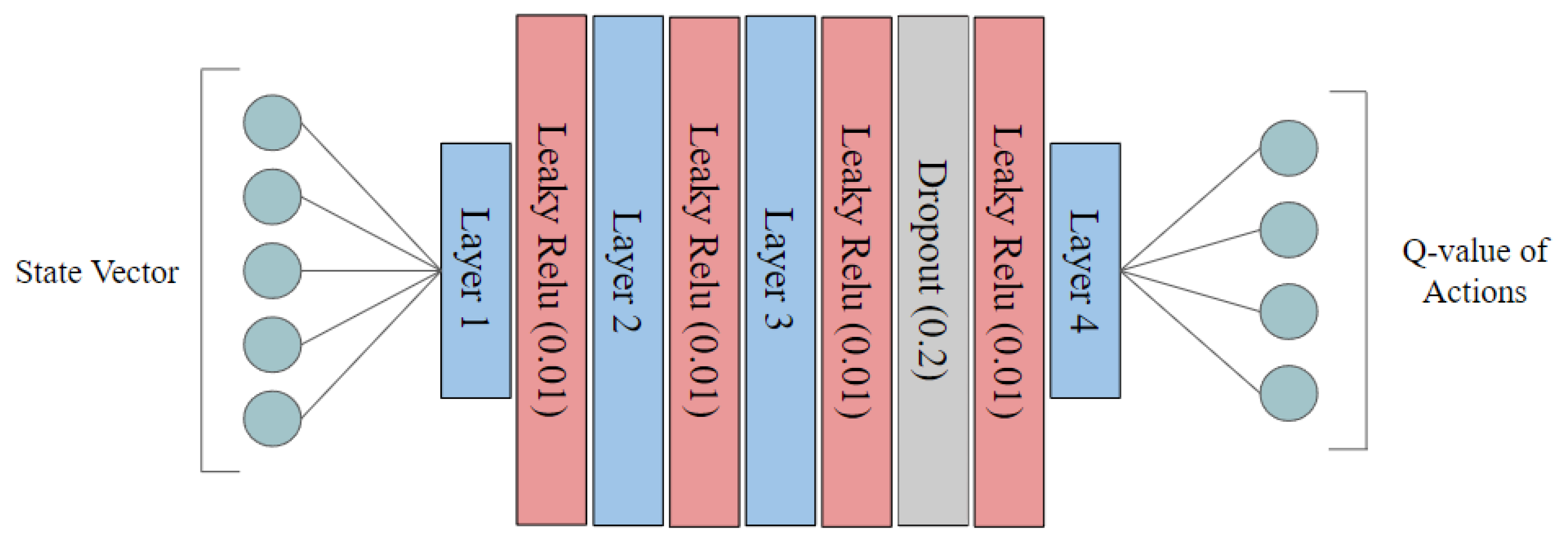
The experiments were carried out on a system equipped with a GTX 1080Ti GPU, an Intel i7-8700k 3.7GHz CPU, and Python 3.7. The environment was managed using Anaconda, with the primary libraries beinggym version 0.19.0 and pytorch version 1.13.1, which were instrumental in creating the RL environment and the neural network, respectively. The neural network model used for the RL agent had 20 and 40 hidden units. The training process utilized a batch size of 32, a learning rate of 0.01, an exploration parameter of 0.2, and a discount factor of 0.9. The target network was updated every 100 iterations and the replay buffer had a capacity of 100. Training was performed on over 100 episodes.

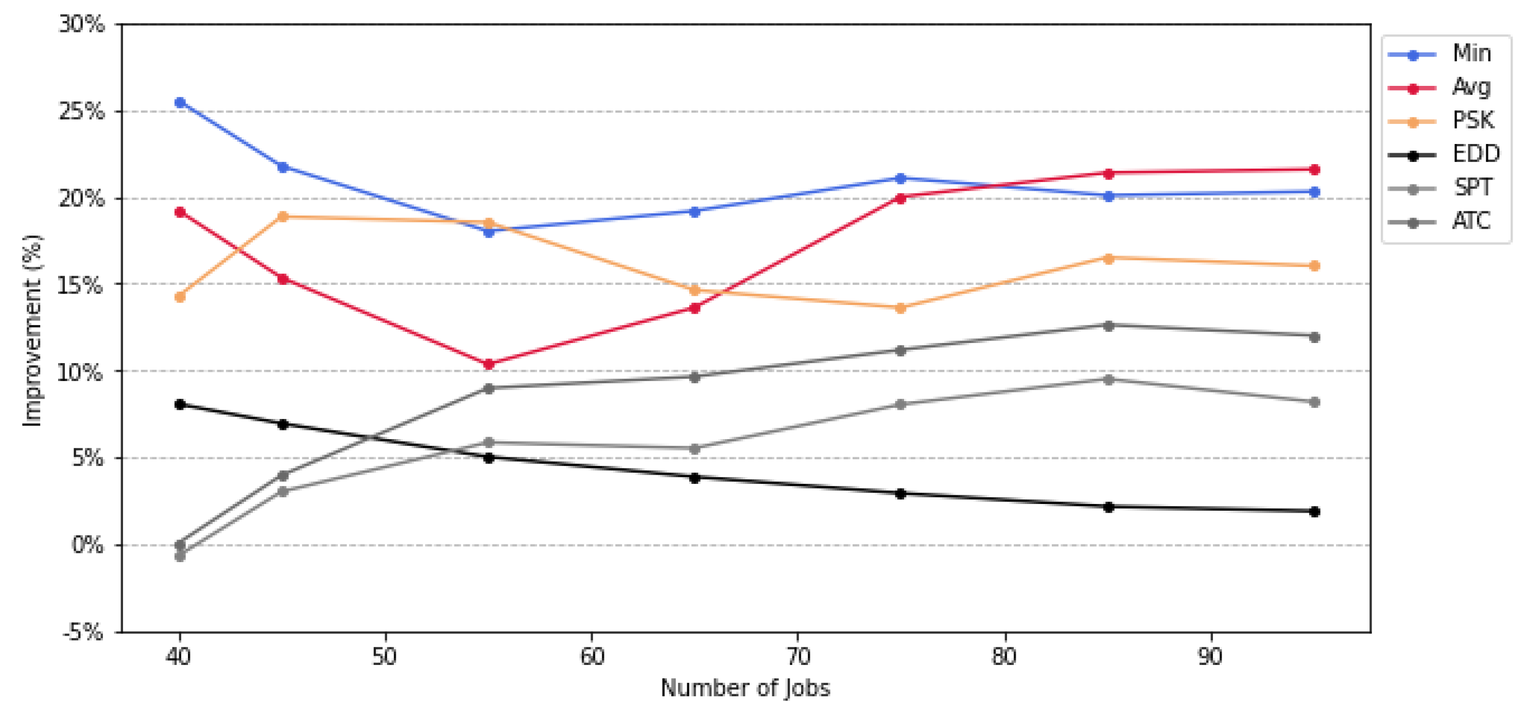
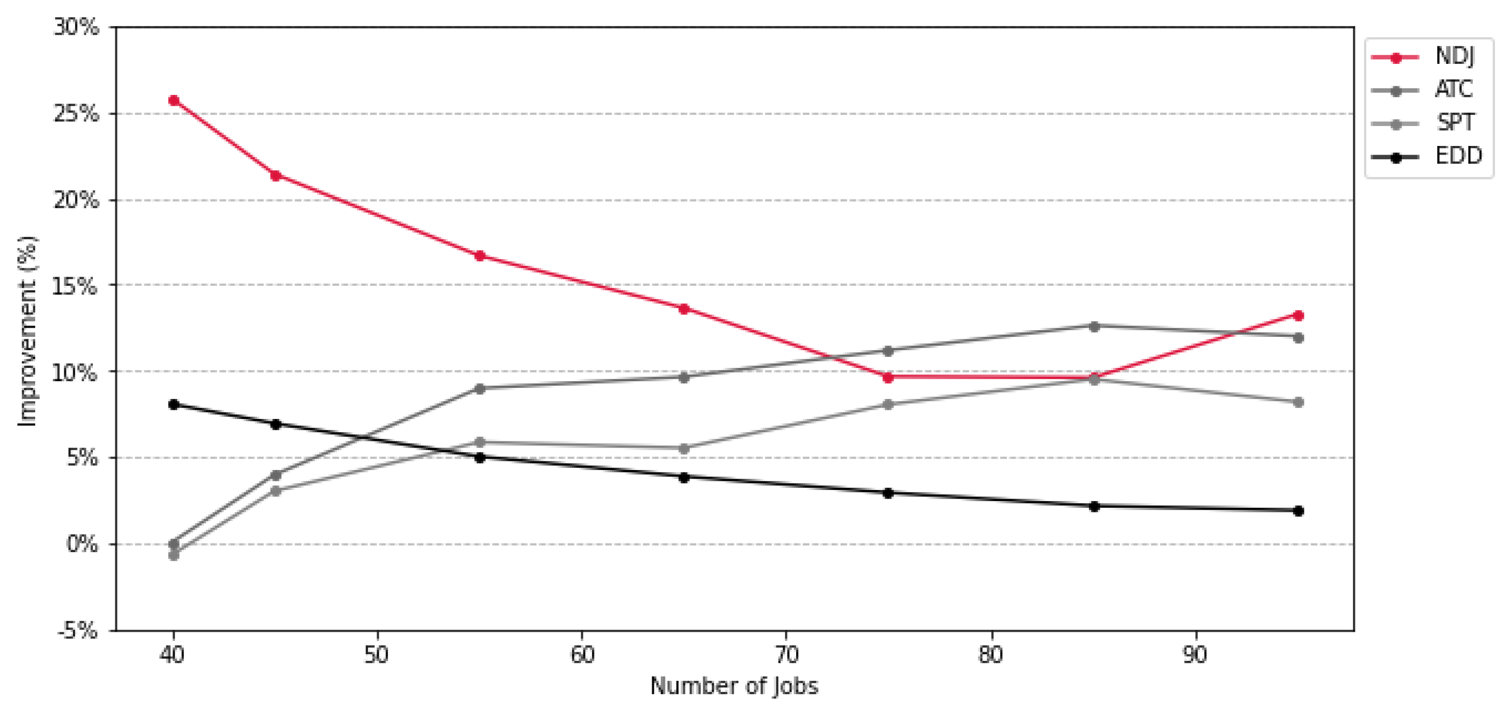
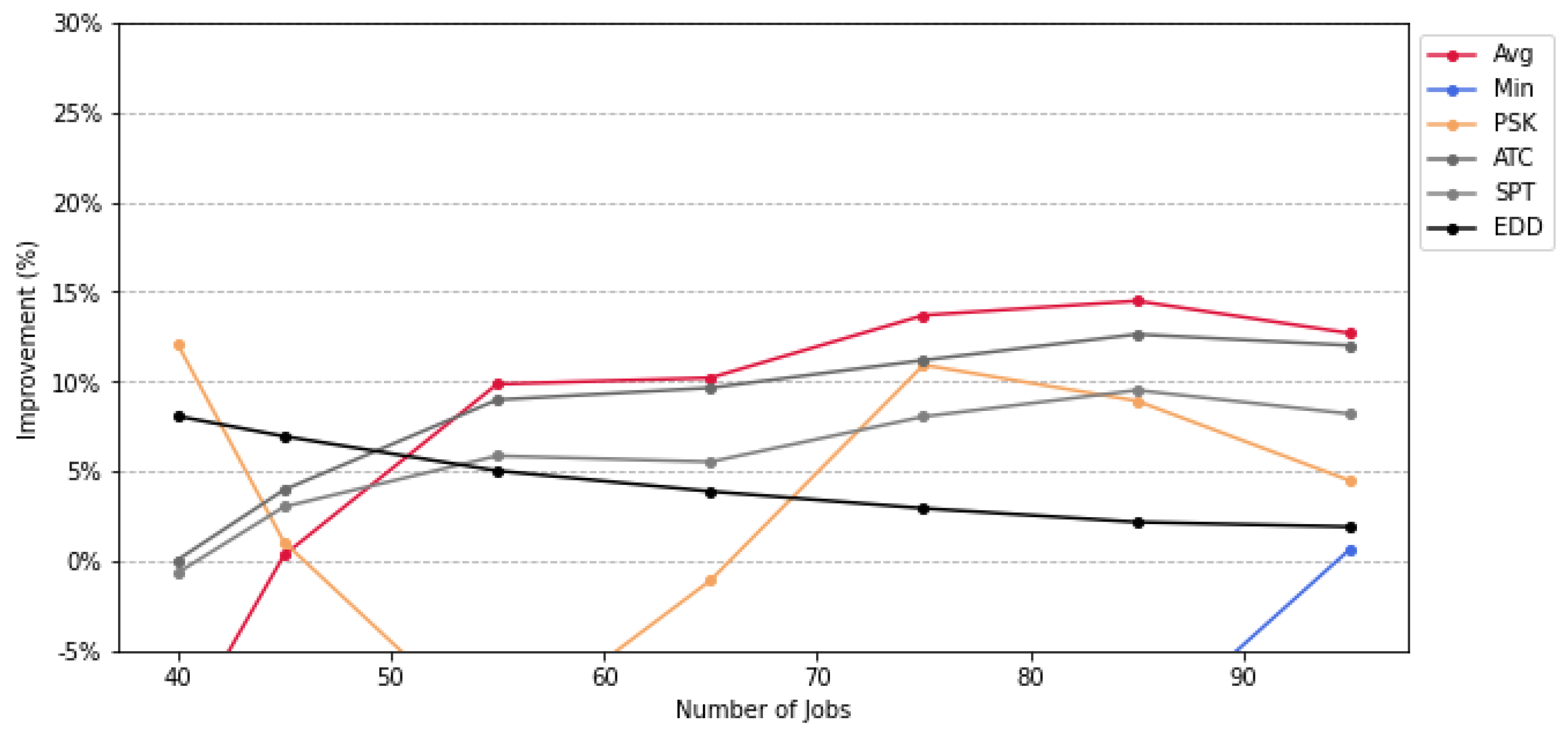
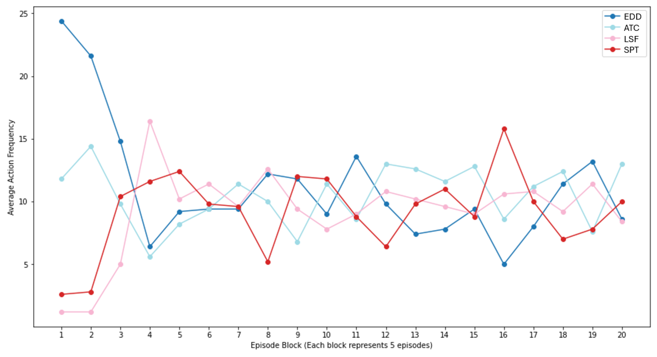
For the experiments, we generated 100 jobs and implemented the DQN using seven different reward strategies. These strategies were compared with four heuristic baselines, i.e., ATC (Apparent Tardiness Cost), EDD (Earliest Due Date), SPT (Shortest Processing Time), and LSF (Least Slack First). We evaluated the final total tardiness of the schedules produced by the DQN and the baselines across a range of job sizes from 40 to 100, in increments of 10 jobs, derived from the generated job set.

5. Results and Analysis

This section presents the computational results along with comparative analysis of various reward strategies and heuristics. The first part compares the machine learning mechanism DQN model with four baseline dispatching heuristics that are commonly adopted in practical applications. The second part further analyzes the performance of the proposed DQN when different reward strategies are embedded into the model. This would be of referential values for designing reward strategies, which play an essential role in machine learning techniques concerning state/action transitions.

5.1. Comparative Analysis

In

Table 6. Total tardiness across DQN and baseline heuristics—Estimated Future Tardiness.

# of Jobs (n)	MIN	AVG	PSK	EDD	SPT	ATC	MST
40	1236	1341	1423	1526	1671	1659	1660
50	2248	2427	2099	2582	2558	2526	2742
60	3451	3822	3637	4033	4000	3786	4211
70	4913	5056	5202	5949	5794	5599	6167
80	6921	6909	7829	8650	7967	7690	8857
90	9614	9322	9248	11,534	10,712	10,346	11,770
100	11,723	11,711	13,483	14,815	13,969	13,287	15,088

, we present a comprehensive comparison between our DQN model employing EFT reward strategies—Minimum (Min), Average (Avg), and the PSK algorithm (PSK)—and four established baseline heuristics: Earliest Due Date (EDD), Least Slack First (LSF), Apparent Tardiness Cost (ATC), and Shortest Processing Time (SPT). In each row (instance size), the entries in boldface indicate the best results among the different methods. This analysis demonstrates the superiority of our DQN model in optimizing job scheduling tasks, consistently outperforming the baseline heuristics across various job counts. We next discuss and analyze the statistics in details.

As the LSF heuristic shows the least effective performance among our baseline methods, it serves as a benchmark for evaluating the enhancement capabilities of other scheduling strategies. Figure 5 illustrates the percentage improvement over the LSF heuristic across a range of job counts, showcasing the efficacy of different reward strategies employed by our DQN model. To enhance clarity and readability, the data have been smoothed using a moving average over every 20 jobs. Within the job range of 40 to 100, the Min strategy emerges as the standout performer, consistently yielding the highest improvements, peaking at 40 jobs with a 25.54% improvement. Conversely, the Avg strategy, while initially falling short of Min, exhibits a noticeable uptrend in performance beyond 80 jobs. This suggests that while Min maintains superior consistency, Avg becomes increasingly effective as the job count escalates, indicating a potential preference for larger-scale job counts. However, PSK displays significant fluctuations within the 40 to 100 job range, achieving impressive gains at certain points but also experiencing lower enhancements relative to the other DQN strategies. This variability indicates that PSK’s performance is less predictable compared to the consistent Min and the steadily improving Avg.

Among the baseline heuristics, a clear trend emerges as the number of jobs increases: both ATC and SPT begin to outshine EDD and LSF. This is particularly evident as the job count grows, with ATC and SPT consistently outperforming LSF. The data underscore ATC and SPT’s superior scalability when faced with larger job counts, affirming their robustness as task complexity escalates.

Figure 6 illustrates the performance trend of the DQN algorithm using the Number of Delayed Jobs (NDJ) reward strategy. The DQN demonstrates an increasing improvement over the baseline heuristics, reaching a peak enhancement of 25.78% at 40 jobs. However, its performance diminishes as the number of jobs exceeds 40, with only a 15.71% improvement observed at 100 jobs. Notably, the DQN is surpassed by the ATC heuristic around 80 jobs. This trend underscores that the effectiveness of the DQN diminishes with heavier workloads.

Figure 7 illustrates the trend in the percentage improvement for the DQN employing a mixed reward strategy of Estimated Future Tardiness (EFT) and Local Job Tardiness (LJT). Compared to strategies solely based on average EFT, which show a steady but modest improvement over baselines, strategies utilizing minimum EFT and the PSK algorithm exhibit significantly poorer performance. Not only do they underperform relative to the average EFT method, but they also fail to surpass baseline levels. It is important to note that some data points exhibit negative improvements that exceed the bottom limit of the y-axis. For a better visualization, the bottom limit of the y-axis is set to −5%. For the complete dataset, please refer to Appendix A.

This outcome can be anticipated given the characteristics of the LJT reward strategy, which focuses exclusively on the tardiness of the individual job selected at each slot. Such a focus may lead to delayed rewards, as the objective value—total tardiness of the complete schedule—is seldom determined by the tardiness of single jobs. This aspect is particularly problematic for jobs positioned in the initial slots of the schedule, where the agent often receives positive rewards due to the jobs’ completion times generally preceding their due dates. However, these positive rewards may not accurately reflect the broader impact of job selection at a specific slot, which could lead to increased tardiness for subsequent jobs, thereby exacerbating the overall tardiness of the schedule. This misalignment highlights the potential pitfalls of reward strategies that do not adequately account for the cumulative effects of individual job placements within the overall task context.

Table 7. Counts of best results achieved by different reward strategies.

EFT & LJT			EFT			# of Delayed Jobs
Avg	Min	PSK	Avg	Min	PSK
0	0	0	0	4	2	1

illustrates the frequency with which each reward strategy achieved the lowest total tardiness across job sizes ranging from 40 to 100. Notably, the strategy that solely employs EFT and the minimum criterion achieved the highest frequency, with a count of four, while the strategies involving EFT with the PSK criterion and the Number of Delayed Jobs each recorded a frequency of one. It is important to note that no strategy that incorporates a combination of LJT and EFT outperformed other strategies in any instance. Although the strategy focusing on the Number of Delayed Jobs outperformed the EFT Min strategy in one specific instance, the overall difference in performance was statistically insignificant. This underscores the robust performance of the EFT Min strategy in our experiments, particularly when considering total tardiness as the sole metric.

Table 8. Training duration for DQN by reward strategy.

# of Jobs n	EFT & LJT			EFT			# of Delayed Jobs
	Avg	Min	PSK	Avg	Min	PSK
40	1046	1152	11	1158	983	11	11
50	1516	1700	14	1752	1471	15	15
60	2119	2353	18	2536	2082	20	20
70	2881	3125	22	3325	2780	25	24
80	3684	4015	26	4337	3823	31	31
90	4975	4948	31	5463	4723	38	32
100	6007	6026	36	6892	5771	44	38

demonstrates the time elapsed for each reward strategy. The results indicate that strategies requiring the computation of EFT with minimum and average criteria are time intensive, as they require extensive sampling through possible schedules. Conversely, strategies based on PSK and the Number of Delayed Jobs require considerably less computation time. Given that the strategy focusing solely on the Number of Delayed Jobs exhibited an average gap of only 3% compared to the EFT with the Min strategy across job sizes from 40 to 100, it can be concluded that the overall performance of this strategy is satisfactory.

5.2. Evaluation of Rewards and Action Distribution

Figure 8 illustrates the trend in action frequencies across 100 episodes for the DQN model utilizing the Method 2A reward strategy, where the EFT is the minimum of the sampled tardiness. The trend is smoothed with a window of five. The figure includes four lines representing four different actions: EDD, SPT, LSF, and ATC. Initially, there are distinctive differences in the frequencies, with EDD having a significantly higher frequency, followed by ATC, then LSF, and finally SPT. This observation is consistent with the data in Table 6, where EDD performs significantly better than the other three heuristics. As episodes progress, the distinctions between the four actions begin to shrink and exhibit fluctuations, indicating a convergence in their usage frequencies over time. Figure 9 presents the episode reward and the total tardiness of the completed schedule at the end of each episode during the training process of Method 2A. The episode reward plot is inverted, as the reward in our RL environment is defined as the negative value of the observed tardiness. The trends in the figure are smoothed using a moving average window of five episodes. A comparison of the two plots reveals a strong alignment in their trends, while both plots show an overall declining trend, they in the meantime exhibit significant fluctuations, which correspond with the variations in action frequencies observed in Figure 8.

Before concluding our discussion on the numerical study, we acknowledge several limitations of our research. First, while we focused on the static single-machine total tardiness problem with pre-defined job attributes such as due dates and processing times, this limits the applicability of the proposed DQN model in dynamic or real-time scheduling scenarios where job attributes may evolve over time, and jobs may spontaneously arrive with various urgencies. Second, we did not implement other existing solution approaches within discrete optimization or machine learning for performance comparisons. Without benchmark datasets for comparing the known performances, implementing these methods from scratch would require substantial effort, and replicating previous designs as described in the literature is challenging, even with known parameter settings. Third, our study assumes deterministic job attributes and excludes complexities like sequence-dependent setup times, stochastic processing times, queue time constraints, or multi-machine environments, which are often encountered in real-world applications. Additionally, while we explored specific reward designs (local, global, and mixed), the generalizability of these approaches to other scheduling contexts remains an open question. Finally, although our numerical study spans a range of job sizes, the scalability of the DQN approach to extremely large or highly complex scheduling environments and its computational cost compared to traditional methods warrant further investigations. These limitations highlight potential directions for extending this work in future studies.

6. Conclusions and Future Work

This study developed a Deep Q-Network (DQN) framework tailored to address the single-machine total tardiness problem for job sizes ranging from 40 to 100. We investigated the effects of deploying heuristics information, local or long-term, on the composition of decent schedules. The framework incorporates seven distinct reward-shaping strategies, among which the Minimum Estimated Future Tardiness strategy notably enhances the DQN model’s performance. Specifically, it achieves an average improvement of 14.33% over Earliest Due Date (EDD), 11.90% over Shortest Processing Time (SPT), 17.65% over Least Slack First (LSF), and 8.86% over Apparent Tardiness Cost (ATC). Conversely, the Number of Delayed Jobs strategy secures an average improvement of 11.56% over EDD, 9.10% over SPT, 15.01% over LSF, and 5.99% over ATC, all while requiring minimal computational resources. Moreover, the study evaluated the limitations of incorporating Local Job Tardiness within the framework, highlighting its potential to overlook long-term impacts. This investigation paves the way for further exploration of DQN applications in managing single-machine total tardiness challenges.

The current Deep Q-Network implementation employs a straightforward architecture, consisting of vanilla feed-forward neural networks with hidden layers, a dropout layer, and Leaky ReLU activation functions. This architecture was selected to match the relatively simple state and action space within our environment. Future research could broaden this scope by extending the problem to encompass multiple machines and integrating job precedence constraints to introduce a more complex state space. Moreover, expanding the range of actionable choices to include various heuristic-based job selections could enrich the model’s decision-making process. Such enhancements might necessitate a more sophisticated neural network architecture to efficiently compute the Q-values, potentially leading to more robust and scalable solutions for complex scheduling problems. We can also consider deploying the same strategies to the simplified models, like Q-learning or Double Q-learning, to examine if more significant performances are achievable.

References

1. Hassan, A.; Triki, H.; Trabelsi, H.; Haddar, M. Literature review of scheduling problems using artificial intelligence technologies based on machine learning. In Design and Modeling of Mechanical Systems-VI: Proceedings of the 10th Conference on Design and Modeling of Mechanical Systems, CMSM’2023, Hammamet, Tunisia, 18–20 December 2023; Volume 1: Mechanical Systems Analysis and Industrial Engineering; Springer Nature: Berlin/Heidelberg, Germany, 2024; p. 341. [Google Scholar]
2. Graham, R.L.; Lawler, E.L.; Lenstra, J.K.; Kan, A.R. Optimization and approximation in deterministic sequencing and scheduling: A survey. Ann. Discret. Math. 1979, 5, 287–326. [Google Scholar]
3. Du, J.; Leung, J.Y.T. Minimizing total tardiness on one machine is NP-hard. Math. Oper. Res. 1990, 15, 483–495. [Google Scholar] [CrossRef]
4. Jiang, W.; Zheng, B.; Sheng, D.; Li, X. A compensation approach for magnetic encoder error based on improved deep belief network algorithm. Sensors Actuators Phys. 2024, 366, 115003. [Google Scholar] [CrossRef]
5. Sun, G.; Xu, Z.; Yu, H.; Chang, V. Dynamic network function provisioning to enable network in box for industrial applications. IEEE Trans. Ind. Inform. 2020, 17, 7155–7164. [Google Scholar] [CrossRef]
6. Zhu, C. An adaptive agent decision model based on deep reinforcement learning and autonomous learning. J. Logist. Inform. Serv. Sci. 2023, 10, 107–118. [Google Scholar]
7. Srinivasan, V. A hybrid algorithm for the one machine sequencing problem to minimize total tardiness. Nav. Res. Logist. Q. 1971, 18, 317–327. [Google Scholar] [CrossRef]
8. Emmons, H. One-machine sequencing to minimize certain functions of job tardiness. Oper. Res. 1969, 17, 701–715. [Google Scholar] [CrossRef]
9. Baker, K.R. Computational experience with a sequencing algorithm adapted to the tardiness problem. AIIE Trans. 1977, 9, 32–35. [Google Scholar] [CrossRef]
10. Lawler, E.L. A “pseudopolynomial” algorithm for sequencing jobs to minimize total tardiness. Ann. Discret. Math. 1977, 1, 331–342. [Google Scholar]
11. Potts, C.N.; Van Wassenhove, L.N. Dynamic programming and decomposition approaches for the single machine total tardiness problem. Eur. J. Oper. Res. 1987, 32, 405–414. [Google Scholar] [CrossRef]
12. Elmaghraby, S.E. The one-machine sequencing problem with delay costs. J. Ind. Eng. 1968, 19, 105–108. [Google Scholar]
13. Shwimer, J. On the N-job one-machine, sequence-independent scheduling problem with tardiness penalties: A branch-bound solution. Manag. Sci. 1972, 18, B-301. [Google Scholar] [CrossRef]
14. Rinnooy Kan, A.H.G.; Lageweg, B.J.; Lenstra, J.K. Minimizing total costs in one-machine scheduling. Oper. Res. 1975, 23, 908–927. [Google Scholar] [CrossRef]
15. Fisher, M.L. A dual algorithm for the one-machine scheduling problem. Math. Program. 1976, 11, 229–251. [Google Scholar] [CrossRef]
16. Picard, J.-C.; Queyranne, M. The time-dependent traveling salesman problem and its application to the tardiness problem in one-machine scheduling. Oper. Res. 1978, 26, 86–110. [Google Scholar] [CrossRef]
17. Sen, T.T.; Austin, L.M.; Ghandforoush, P. An algorithm for the single-machine sequencing problem to minimize total tardiness. AIIE Trans. 1983, 15, 363–366. [Google Scholar] [CrossRef]
18. Baker, K.R.; Bertrand, J.W.M. A dynamic priority rule for scheduling against due-dates. J. Oper. Manag. 1982, 3, 37–42. [Google Scholar] [CrossRef]
19. Carroll, D.C. Heuristic Sequencing of Single and Multiple Component Jobs. Ph.D. Thesis, Massachusetts Institute of Technology, Cambridge, MA, USA, 1965. [Google Scholar]
20. Rachamadugu, R.M.V.; Morton, T.E. Myopic Heuristics for the Weighted Tardiness Problem on Identical Parallel Machines; Working Paper No. 371; University of Michigan: Ann Arbor, MI, USA; Carnegie-Melon University: Pittsburgh, PA, USA, 1983. [Google Scholar]
21. Panwalkar, S.S.; Smith, M.L.; Koulamas, C.P. A heuristic for the single machine tardiness problem. Eur. J. Oper. Res. 1993, 70, 304–310. [Google Scholar] [CrossRef]
22. Naidu, J.T. Some properties of the optimal decomposition conditions for the single machine tardiness problem. Am. J. Manag. 2024, 24, 9–16. [Google Scholar] [CrossRef]
23. Fry, T.D.; Vicens, L.; Macleod, K.; Fernandez, S. A heuristic solution procedure to minimize T on a single machine. J. Oper. Res. Soc. 1989, 40, 293–297. [Google Scholar]
24. Holsenback, J.E.; Russell, R.M. A heuristic algorithm for sequencing on one machine to minimize total tardiness. J. Oper. Res. Soc. 1992, 43, 53–62. [Google Scholar] [CrossRef]
25. Wilkerson, L.J.; Irwin, J.D. An improved method for scheduling independent tasks. AIIE Trans. 1971, 3, 239–245. [Google Scholar] [CrossRef]
26. Ho, J.C.; Chang, Y.-L. Heuristics for minimizing mean tardiness for m parallel machines. Nav. Res. Logist. 1991, 38, 367–381. [Google Scholar] [CrossRef]
27. Potts, C.N.; Van Wassenhove, L.N. Single machine tardiness sequencing heuristics. IIE Trans. 1991, 23, 346–354. [Google Scholar] [CrossRef]
28. Koulamas, C. The total tardiness problem: Review and extensions. Oper. Res. 1994, 42, 1025–1041. [Google Scholar] [CrossRef]
29. Wang, Y.-C.; Usher, J.M. Learning policies for single machine job dispatching. Robot. Comput. Integr. Manuf. 2004, 20, 553–562. [Google Scholar] [CrossRef]
30. Kong, L.-F.; Wu, J. Dynamic single machine scheduling using Q-learning agent. In Proceedings of the 2005 International Conference on Machine Learning and Cybernetics, Guangzhou, China, 18 August 2005; IEEE: Piscataway, NJ, USA, 2005; Volume 5, pp. 3237–3241. [Google Scholar]
31. Idrees, H.D.; Sinnokrot, M.O.; Al-Shihabi, S. A reinforcement learning algorithm to minimize the mean tardiness of a single machine with controlled capacity. In Proceedings of the 2006 Winter Simulation Conference, Monterey, CA, USA, 3 December 2006; IEEE: Piscataway, NJ, USA, 2006; pp. 1765–1769. [Google Scholar]
32. Xanthopoulos, A.S.; Koulouriotis, D.E.; Tourassis, V.D.; Emiris, D.M. Intelligent controllers for bi-objective dynamic scheduling on a single machine with sequence-dependent setups. Appl. Soft Comput. 2013, 13, 4704–4717. [Google Scholar] [CrossRef]
33. Li, Y.; Fadda, E.; Manerba, D.; Tadei, R.; Terzo, O. Reinforcement learning algorithms for online single-machine scheduling. In Proceedings of the 15th Conference on Computer Science and Information Systems (FedCSIS), Sofia, Bulgaria, 6–9 December 2020; IEEE: Piscataway, NJ, USA, 2020; pp. 277–283. [Google Scholar]
34. Bouška, M.; Šůcha, P.; Novák, A.; Hanzálek, Z. Deep learning-driven scheduling algorithm for a single machine problem minimizing the total tardiness. Eur. J. Oper. Res. 2023, 308, 990–1006. [Google Scholar] [CrossRef]
35. Della Croce, F.; Tadei, R.; Baracco, P.; Grosso, A. A new decomposition approach for the single machine total tardiness scheduling problem. J. Oper. Res. Soc. 1989, 49, 1101–1106. [Google Scholar] [CrossRef]
36. Kayhan, B.M.; Yildiz, G. Reinforcement learning applications to machine scheduling problems: A comprehensive literature review. J. Intell. Manuf. 2023, 34, 905–929. [Google Scholar] [CrossRef]
37. Bellman, R.E.; Dreyfus, S.E. Applied Dynamic Programming; Princeton University Press: Princeton, NJ, USA, 2015. [Google Scholar]
38. Watkins, C.J.C.H. Learning from Delayed Rewards. Ph.D. Thesis, Cambridge University, Cambridge, UK, 1989. [Google Scholar]
39. Hall, N.G.; Posner, M.E. Generating experimental data for computational testing with machine scheduling applications. Oper. Res. 2001, 49, 854–865. [Google Scholar] [CrossRef]
Figure 2. Neural network for both target and evaluation networks.
Mathematics 13 00062 g002
Figure 3. Flowchart of the DQN model.
Mathematics 13 00062 g003
Figure 5. Improvement over LSF baseline−EFT.
Mathematics 13 00062 g005
Figure 6. Improvement over LSF baseline−Number of Delayed Jobs.
Mathematics 13 00062 g006
Figure 7. Improvement over LSF baseline−EFT & LJT.
Mathematics 13 00062 g007
Figure 8. Action frequencies across episodes—40 jobs.
Mathematics 13 00062 g008
Figure 9. Rewards and total tardiness across episodes—40 jobs.
Mathematics 13 00062 g009