

A New Fault Diagnosis Method for Rolling Bearings with the Basis of Swin Transformer and Generalized S Transform

Abstract
1. Introduction
2. Materials and Methods
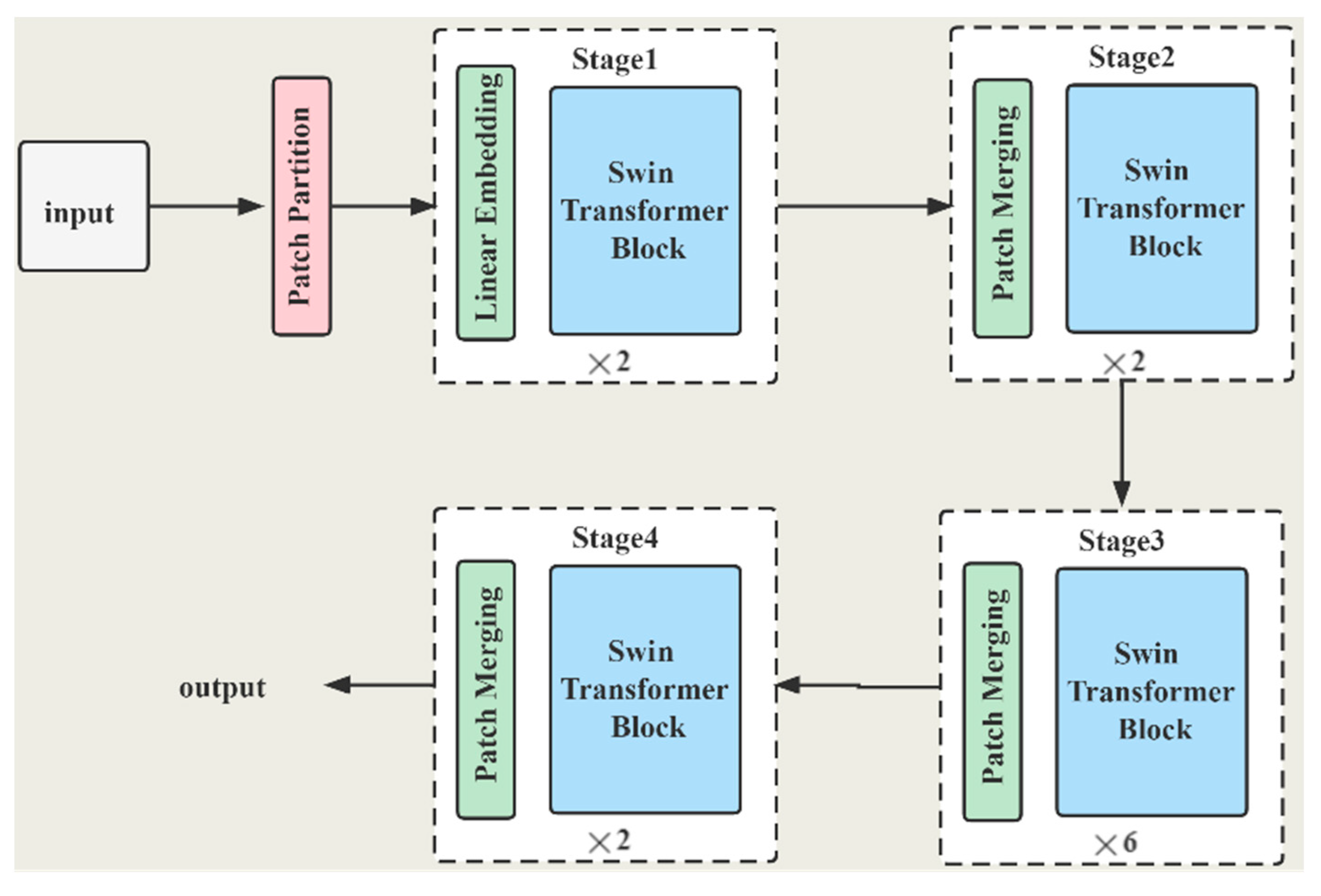
2.1. Swin Transformer
- 1.
- Patch Merging
- 2.
- Swin Transformer Block
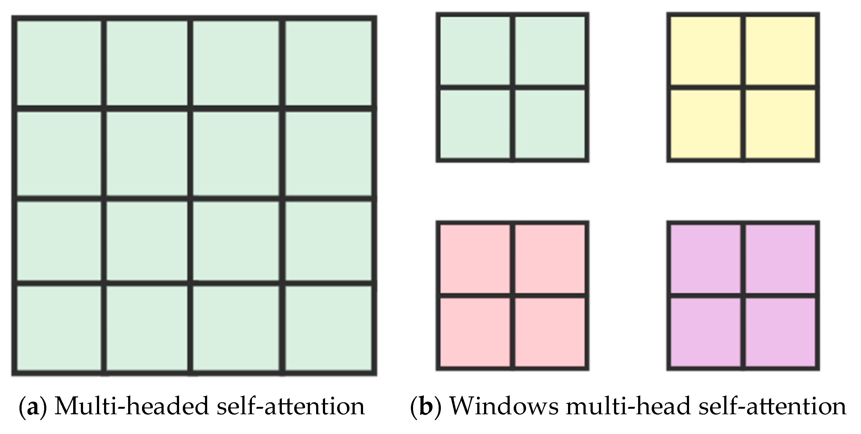
- Multi-head self-attention mechanism
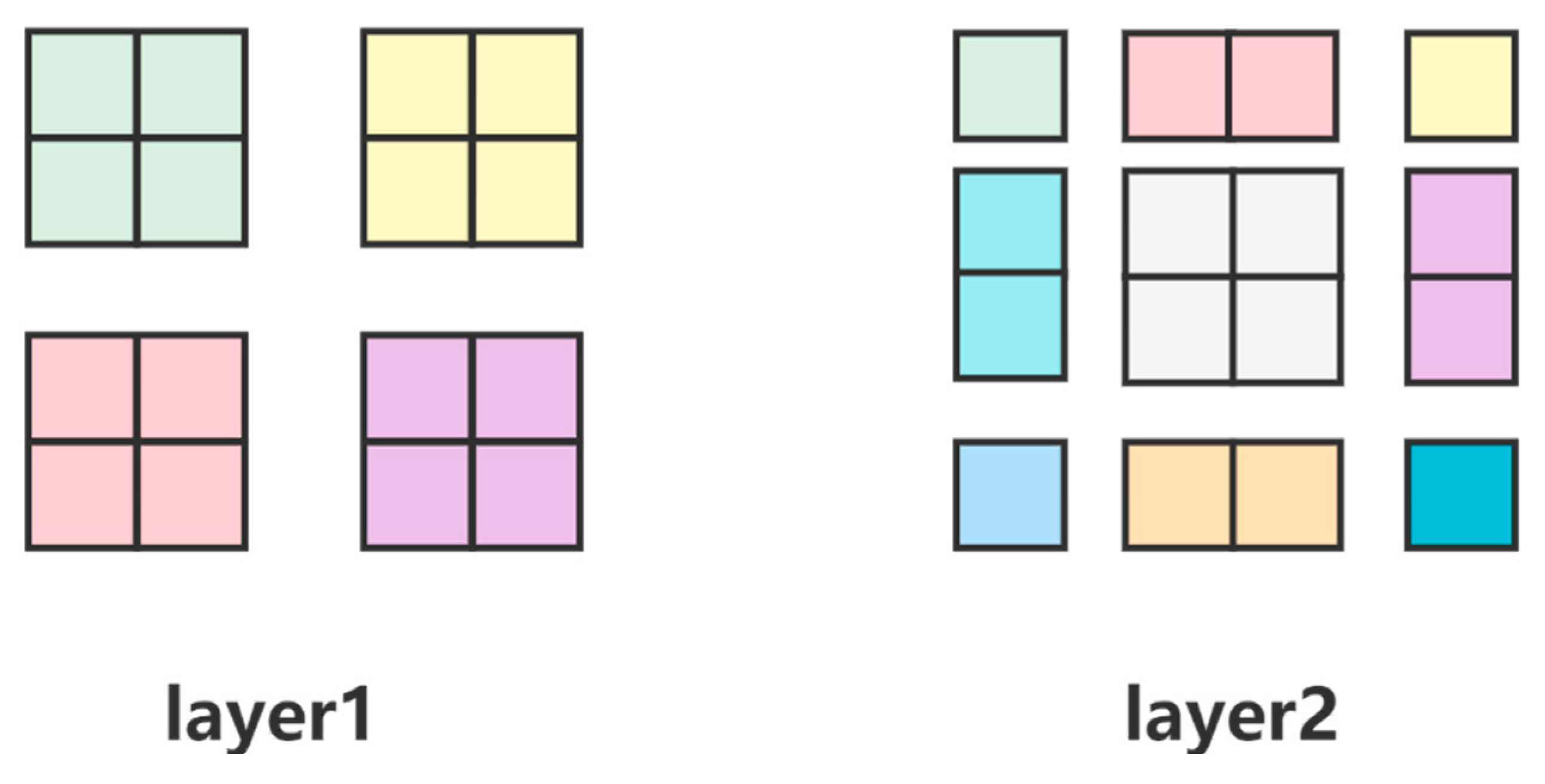
- Offset window self-attention mechanism (SW-MSA)
2.2. Multi-Classification Algorithm
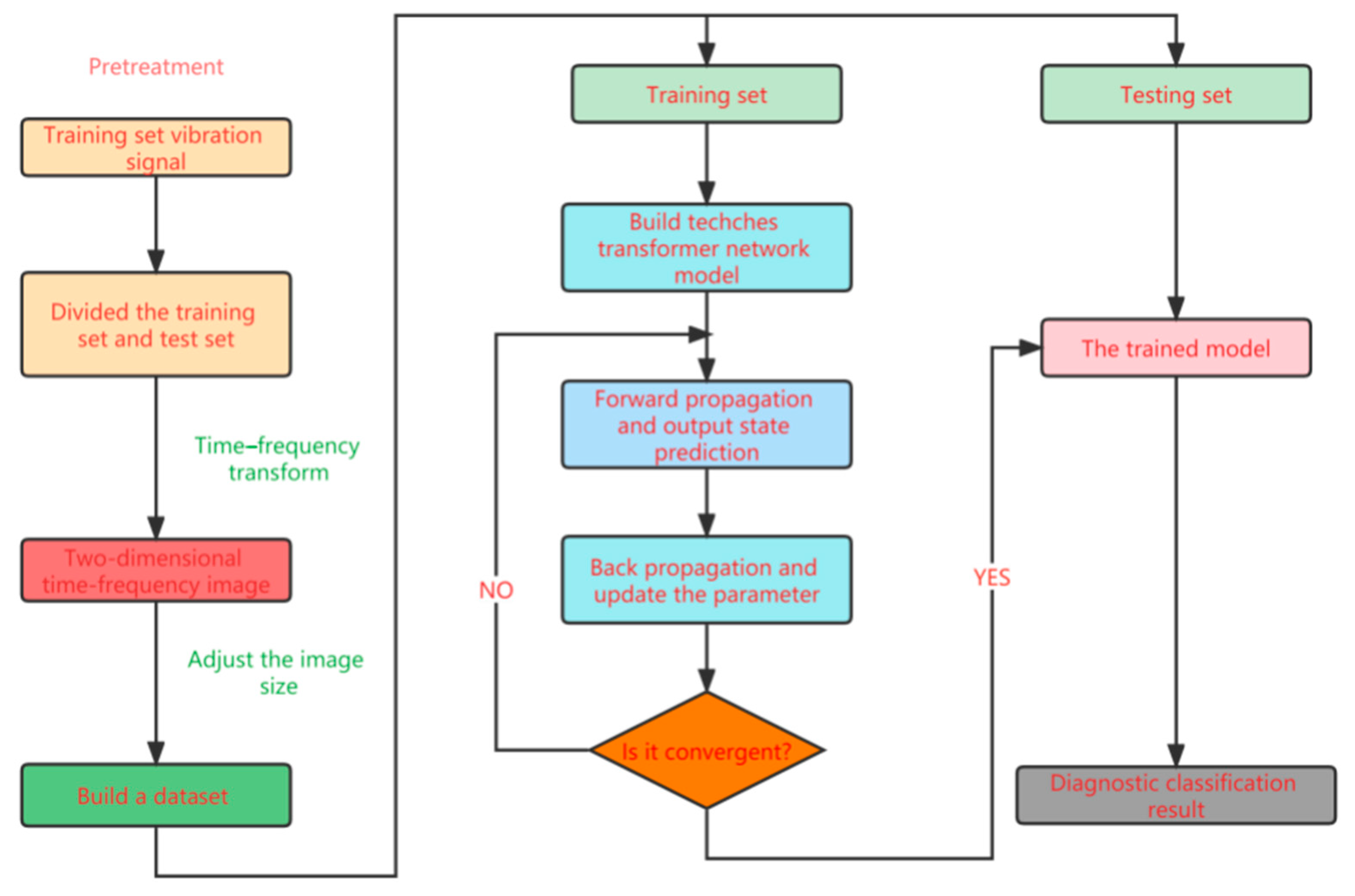
2.3. Troubleshooting Process
3. Results
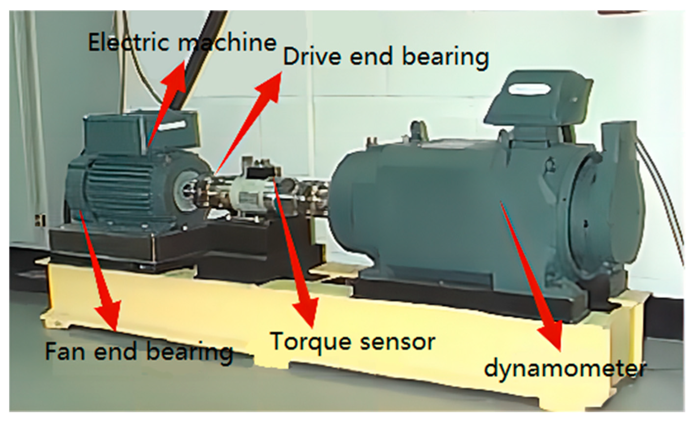
3.1. Experimental Data
3.2. Comparison and Analysis of Time–Frequency Analysis Approaches
- (i)
- Short-time Fourier analysis
- (ii)
- Continuous wavelet transform
- (iii)
- Generalized S transform
- (iv)
- Wigner–Ville distribution
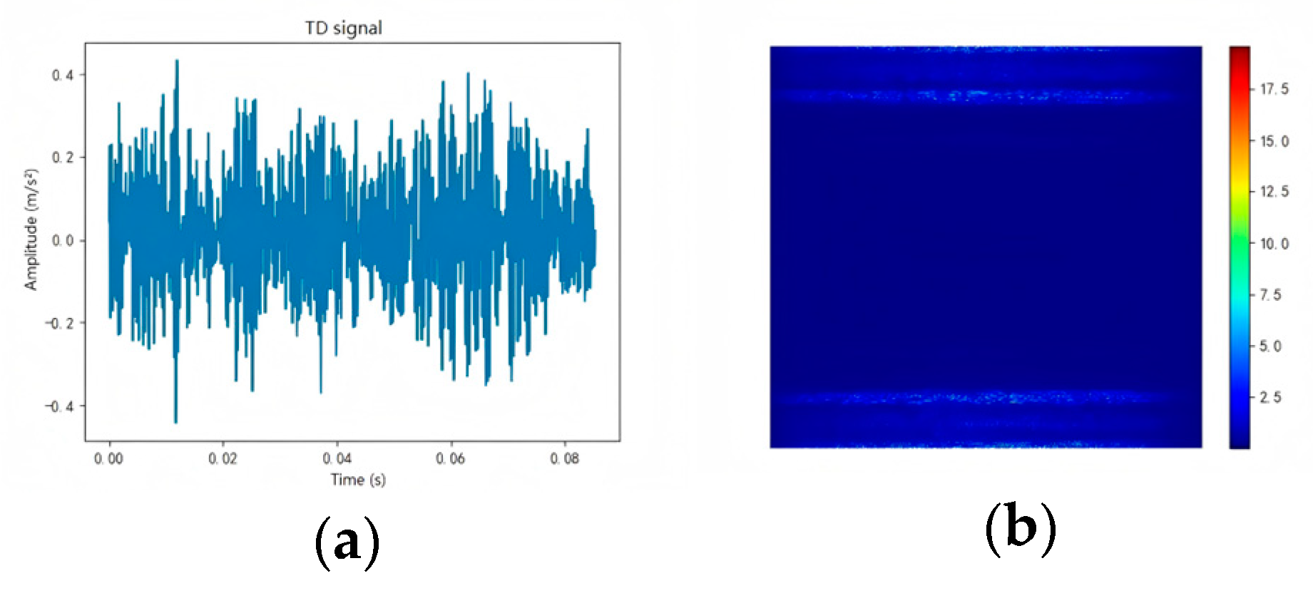
3.3. Data Preprocessing
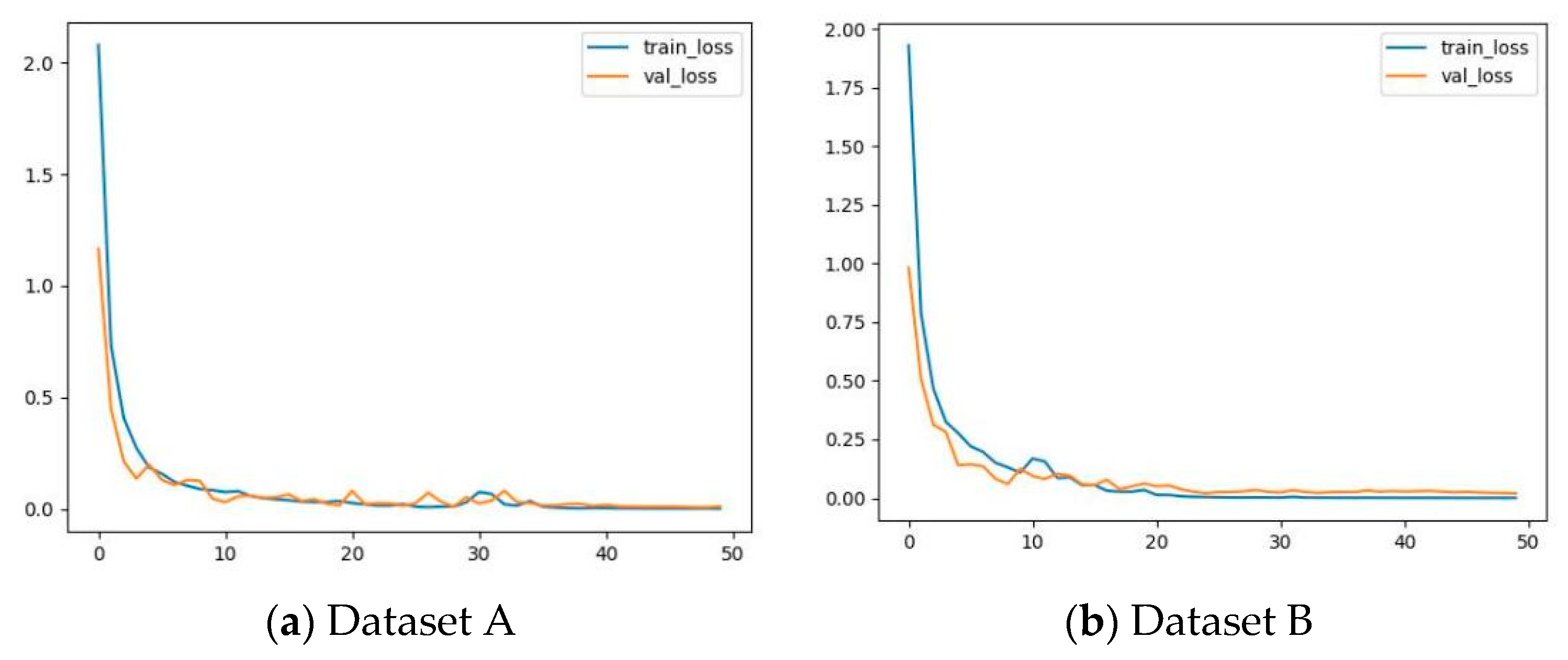
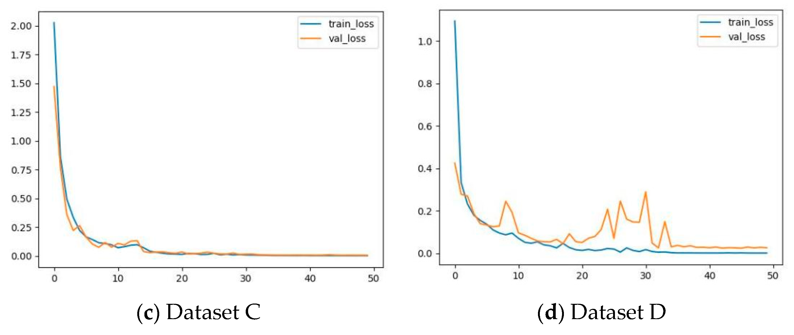
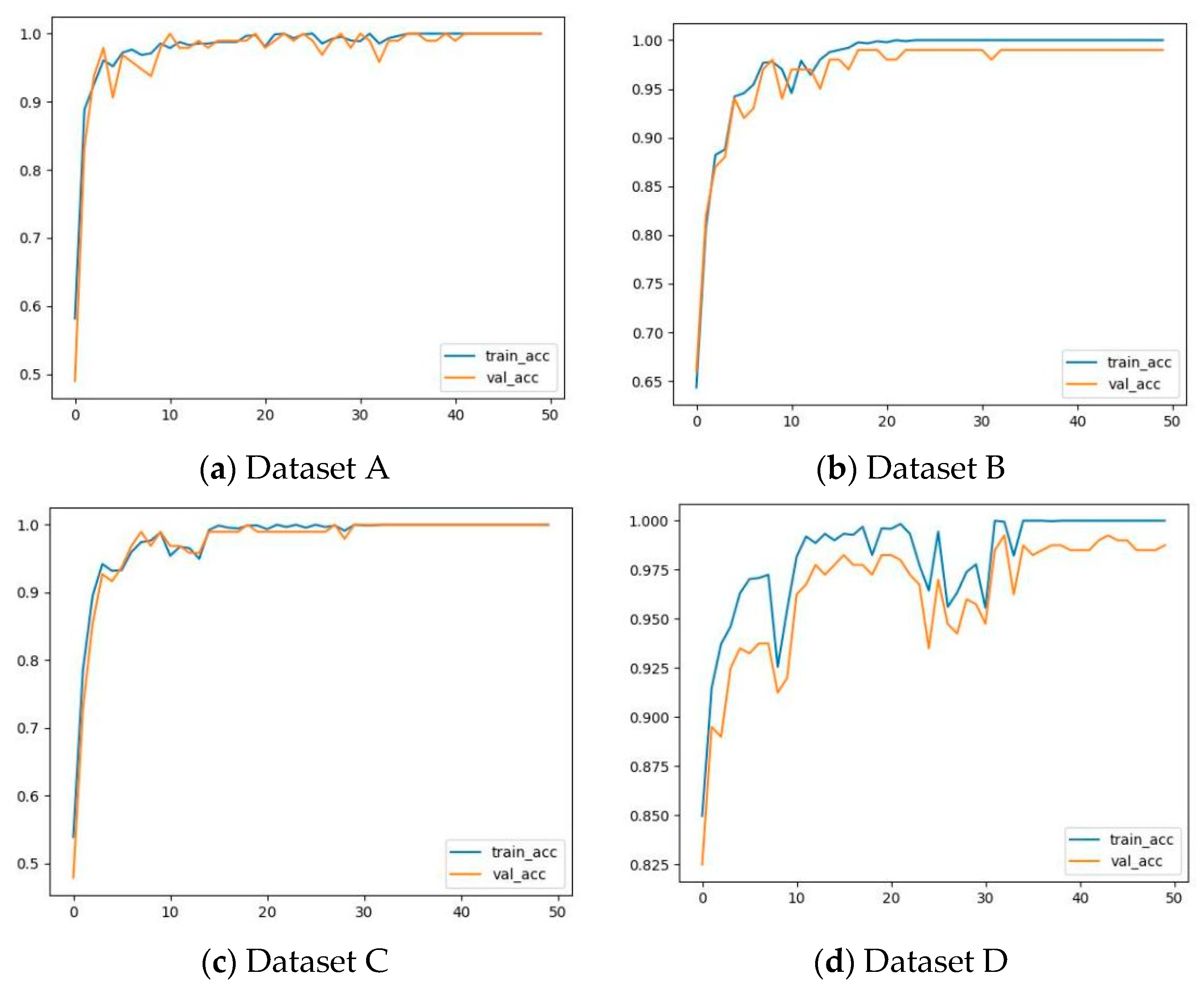
3.4. Experimental Verification
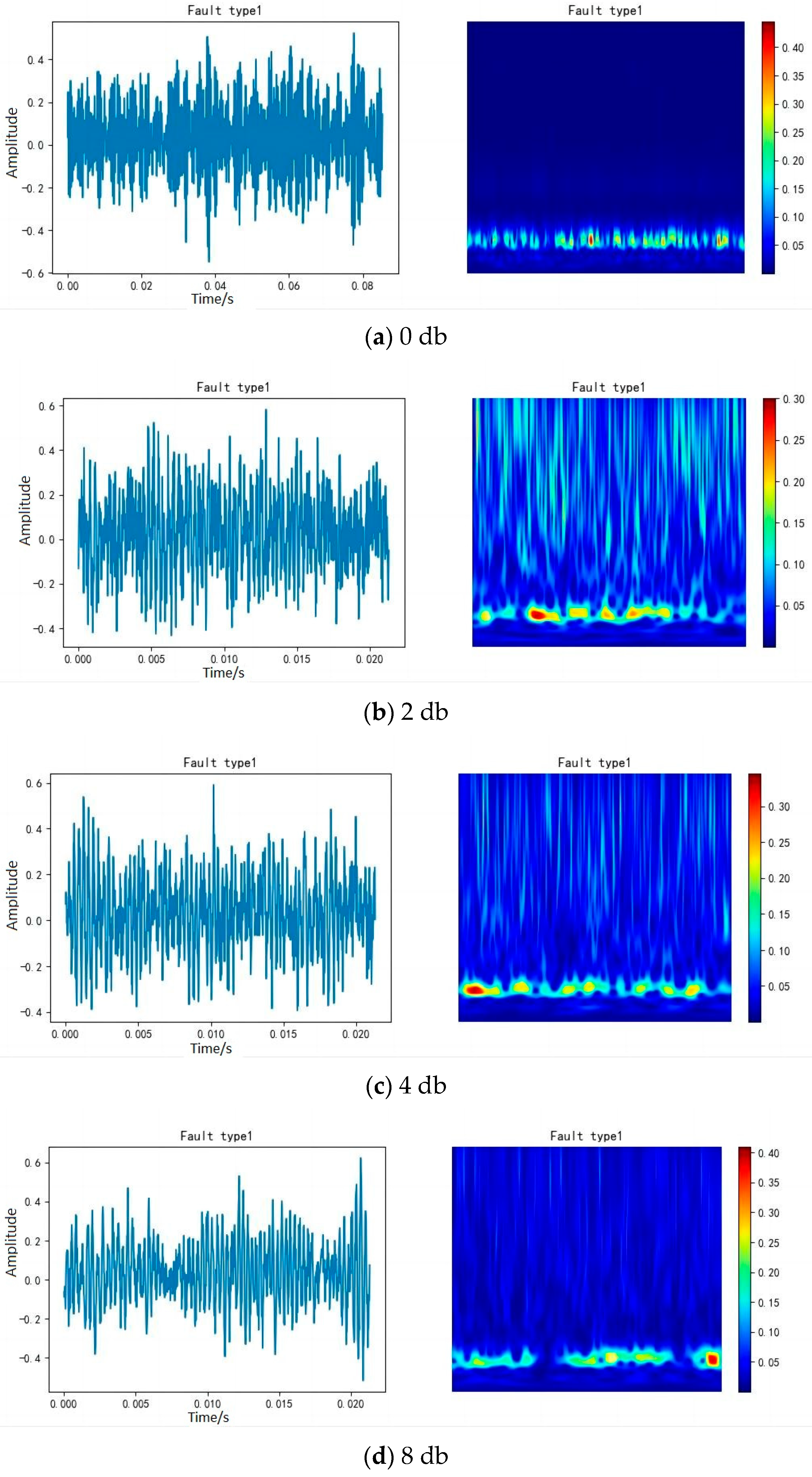
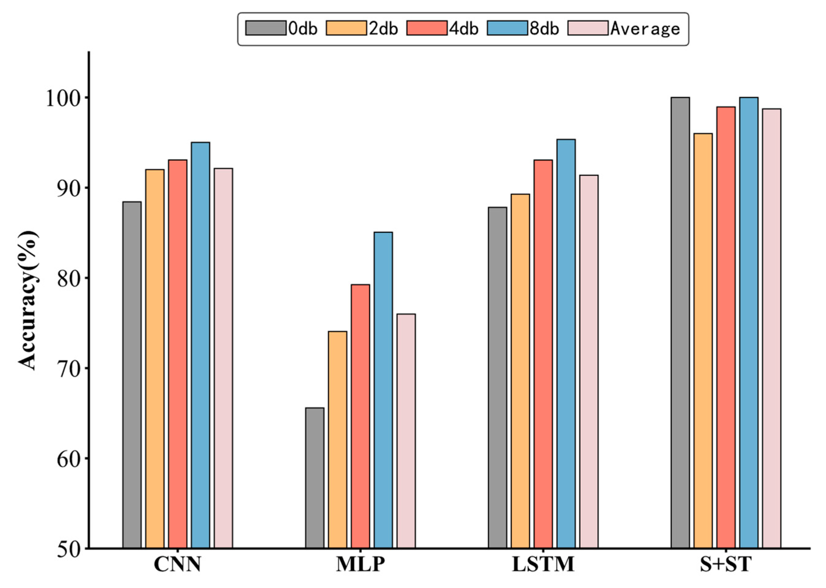
4. Analysis of the Impact of Noise on Model Performance
5. Conclusions
Author Contributions
Funding
Data Availability Statement
Conflicts of Interest
References
- Coutinho, R.W.; Boukerche, A. Modeling and Analysis of a Shared Edge Caching System for Connected Cars and Industrial IoT-Based Applications. IEEE Trans. Ind. Inform. 2019, 16, 2003–2012. [Google Scholar] [CrossRef]
- Li, C.; De Oliveira, J.V.; Cerrada, M.; Cabrera, D.; Sánchez, R.V.; Zurita, G. A Systematic Review of Fuzzy Formalisms for Bearing Fault Diagnosis. IEEE Trans. Fuzzy Syst. 2018, 27, 1362–1382. [Google Scholar] [CrossRef]
- Pacheco-Chérrez, J.; Fortoul-Díaz, J.A.; Cortés-Santacruz, F.; Aloso-Valerdi, L.M.; Ibarra-Zarate, D.I. Bearing Fault Detection with Vibration and Acoustic Signals: Comparison among Different Machine Leaning Classification Methods. Eng. Fail. Anal. 2022, 139, 106515. [Google Scholar] [CrossRef]
- Mian, T.; Choudhary, A.; Fatima, S. An Efficient Diagnosis Approach for Bearing Faults Using Sound Quality Metrics. Appl. Acoust. 2022, 195, 108839. [Google Scholar] [CrossRef]
- Sadegh, H.; Mehdi, A.N.; Mehdi, A. Classification of Acoustic Emission Signals Generated from Journal Bearing at Different Lubrication Conditions Based on Wavelet Analysis in Combination with Artificial Neural Network and Genetic Algorithm. Tribol. Int. 2016, 95, 426–434. [Google Scholar] [CrossRef]
- Motahari-Nezhad, M.; Jafari, S.M. Experimental and Data Driven Measurement of Engine Dynamometer Bearing Lifespan Using Acoustic Emission. Appl. Acoust. 2023, 210, 109460. [Google Scholar] [CrossRef]
- Wen, L.; Li, X.; Gao, L.; Zhang, Y. A New Convolutional Neural Network-Based Data-Driven Fault Diagnosis Method. IEEE Trans. Ind. Electron. 2017, 65, 5990–5998. [Google Scholar] [CrossRef]
- Gong, W.; Wang, Y.; Zhang, M.; Mihankhah, E.; Chen, H.; Wang, D. A Fast Anomaly Diagnosis Approach Based on Modified CNN and Multisensor Data Fusion. IEEE Trans. Ind. Electron. 2021, 69, 13636–13646. [Google Scholar] [CrossRef]
- Liu, R.; Yang, B.; Zio, E.; Chen, X. Artificial Intelligence for Fault Diagnosis of Rotating Machinery: A Review. Mech. Syst. Signal Process. 2018, 108, 33–47. [Google Scholar] [CrossRef]
- Shao, S.; McAleer, S.; Yan, R.; Baldi, P. Highly Accurate Machine Fault Diagnosis Using Deep Transfer Learning. IEEE Trans. Ind. Inform. 2018, 15, 2446–2455. [Google Scholar] [CrossRef]
- Li-Hua, W.; Xiao-Ping, Z.; Jia-Xin, W.; Yang-Yang, X.; Yong-Hong, Z. Motor Fault Diagnosis Based on Short-Time Fourier Transform and Convolutional Neural Network. Chin. J. Mech. Eng. Ji Xie Gong Cheng Xue Bao 2017, 30, 1357–1368. [Google Scholar]
- Jalayer, M.; Orsenigo, C.; Vercellis, C. Fault Detection and Diagnosis for Rotating Machinery: A Model Based on Convolutional LSTM, Fast Fourier and Continuous Wavelet Transforms. Comput. Ind. 2021, 125, 103378. [Google Scholar] [CrossRef]
- Xu, C.; Yang, J.; Zhang, T.; Li, K.; Zhang, K. Adaptive Parameter Selection Variational Mode Decomposition Based on a Novel Hybrid Entropy and Its Applications in Locomotive Bearing Diagnosis. Measurement 2023, 217, 113110. [Google Scholar] [CrossRef]
- Jegadeeshwaran, R.; Sugumaran, V. Fault Diagnosis of Automobile Hydraulic Brake System Using Statistical Features and Support Vector Machines. Mech. Syst. Signal Process. 2015, 52, 436–446. [Google Scholar] [CrossRef]
- Muruganatham, B.; Sanjith, M.A.; Krishnakumar, B.; Murty, S.S. Roller Element Bearing Fault Diagnosis Using Singular Spectrum Analysis. Mech. Syst. Signal Process. 2013, 35, 150–166. [Google Scholar] [CrossRef]
- Zhou, K.; Tang, J. A Wavelet Neural Network Informed by Time-Domain Signal Preprocessing for Bearing Remaining Useful Life Prediction. Appl. Math. Model. 2023, 122, 220–241. [Google Scholar] [CrossRef]
- Wei, B.; Xie, B.; Li, H.; Zhong, Z.; You, Y. An Improved Hilbert–Huang Transform Method for Modal Parameter Identification of a High Arch Dam. Appl. Math. Model. 2021, 91, 297–310. [Google Scholar] [CrossRef]
- Zhang, W.; Li, C.; Peng, G.; Chen, Y.; Zhang, Z. A Deep Convolutional Neural Network with New Training Methods for Bearing Fault Diagnosis under Noisy Environment and Different Working Load. Mech. Syst. Signal Process. 2018, 100, 439–453. [Google Scholar] [CrossRef]
- Fuan, W.; Hongkai, J.; Haidong, S.; Wenjing, D.; Shuaipeng, W. An Adaptive Deep Convolutional Neural Network for Rolling Bearing Fault Diagnosis. Meas. Sci. Technol. 2017, 28, 095005. [Google Scholar] [CrossRef]
- Eren, L.; Ince, T.; Kiranyaz, S. A Generic Intelligent Bearing Fault Diagnosis System Using Compact Adaptive 1D CNN Classifier. J. Signal Process. Syst. 2019, 91, 179–189. [Google Scholar] [CrossRef]
- Xia, M.; Li, T.; Xu, L.; Liu, L.; De Silva, C.W. Fault Diagnosis for Rotating Machinery Using Multiple Sensors and Convolutional Neural Networks. IEEE/ASME Trans. Mechatron. 2017, 23, 101–110. [Google Scholar] [CrossRef]
- Zhao, X.; Yao, J.; Deng, W.; Jia, M.; Liu, Z. Normalized Conditional Variational Auto-Encoder with Adaptive Focal Loss for Imbalanced Fault Diagnosis of Bearing-Rotor System. Mech. Syst. Signal Process. 2022, 170, 108826. [Google Scholar] [CrossRef]
- Wang, D.; Zhang, M.; Xu, Y.; Lu, W.; Yang, J.; Zhang, T. Metric-Based Meta-Learning Model for Few-Shot Fault Diagnosis under Multiple Limited Data Conditions. Mech. Syst. Signal Process. 2021, 155, 107510. [Google Scholar] [CrossRef]
- Su, H.; Xiang, L.; Hu, A.; Xu, Y.; Yang, X. A Novel Method Based on Meta-Learning for Bearing Fault Diagnosis with Small Sample Learning under Different Working Conditions. Mech. Syst. Signal Process. 2022, 169, 108765. [Google Scholar] [CrossRef]
- Li, X.J.; Yang, D.L.; Jiang, L.L. Bearing Fault Diagnosis Based on Multi-Sensor Information Fusion with SVM. Appl. Mech. Mater. 2010, 34, 995–999. [Google Scholar] [CrossRef]
- Ding, X.; He, Q.; Shao, Y.; Huang, W. Transient Feature Extraction Based on Time–Frequency Manifold Image Synthesis for Machinery Fault Diagnosis. IEEE Trans. Instrum. Meas. 2019, 68, 4242–4252. [Google Scholar] [CrossRef]
- Ville, J. Theorie et Application Dela Notion de Signal Analysis. Câbles Transm. 1948, 2, 61–74. [Google Scholar]
- Abboud, D.; Antoni, J.; Sieg-Zieba, S.; Eltabach, M. Envelope Analysis of Rotating Machine Vibrations in Variable Speed Conditions: A Comprehensive Treatment. Mech. Syst. Signal Process. 2017, 84, 200–226. [Google Scholar] [CrossRef]
- Vin Koay, H.; Huang Chuah, J.; Chow, C.-O. Shifted-Window Hierarchical Vision Transformer for Distracted Driver Detection. In Proceedings of the 2021 IEEE Region 10 Symposium (TENSYMP), Jeju, Republic of Korea, 23–25 August 2021; pp. 1–7. [Google Scholar]
- Vaswani, A.; Shazeer, N.; Parmar, N.; Uszkoreit, J. Attention Is All You Need. In Proceedings of the Advances in Neural Information Processing Systems 30 (NIPS 2017), Long Beach, CA, USA, 4–9 December 2017; pp. 5998–6008. [Google Scholar]
- Yao, Y.; Zou, J.; Wang, H. Model Constraints Independent Optimal Subsampling Probabilities for Softmax Regression. J. Stat. Plan. Inference 2023, 225, 188–201. [Google Scholar] [CrossRef]
- Kumar, H.S.; Gururaj, U. Fault Diagnosis of Rolling Element Bearing Using Continuous Wavelet Transform and K- Nearest Neighbour. Mater. Today Proc. 2023, 92, 56–60. [Google Scholar] [CrossRef]
- Bai, R.; Meng, Z.; Xu, Q.; Fan, F. Fractional Fourier and Time Domain Recurrence Plot Fusion Combining Convolutional Neural Network for Bearing Fault Diagnosis under Variable Working Conditions. Reliab. Eng. Syst. Saf. 2023, 232, 109076. [Google Scholar] [CrossRef]
- Yuan, P.-P.; Zhang, J.; Feng, J.-Q.; Wang, H.-H.; Ren, W.-X.; Wang, C. An Improved Time-Frequency Analysis Method for Structural Instantaneous Frequency Identification Based on Generalized S-Transform and Synchroextracting Transform. Eng. Struct. 2022, 252, 113657. [Google Scholar] [CrossRef]
- Mirzaeian, R.; Ghaderyan, P. Gray-Level Co-Occurrence Matrix of Smooth Pseudo Wigner-Ville Distribution for Cognitive Workload Estimation. Biocybern. Biomed. Eng. 2023, 43, 261–278. [Google Scholar] [CrossRef]
- Talebitooti, R.; Zarastvand, M.R.; Gheibi, M.R. Acoustic transmission through laminated composite cylindrical shell employing Third order Shear Deformation Theory in the presence of subsonic flow. Compos. Struct. 2016, 157, 95–110. [Google Scholar] [CrossRef]


| Damage Position | Normal | Inner Ring | Outer Ring | Rolling Element | Load | |||||||
|---|---|---|---|---|---|---|---|---|---|---|---|---|
| Label | 0 | 1 | 2 | 3 | 4 | 5 | 6 | 7 | 8 | 9 | ||
| Damage diameter | 0 | 0.007 | 0.014 | 0.021 | 0.007 | 0.014 | 0.021 | 0.007 | 0.014 | 0.021 | ||
| A | Training | 900 | 900 | 900 | 900 | 900 | 900 | 900 | 900 | 900 | 900 | 0 |
| Testing | 100 | 100 | 100 | 100 | 100 | 100 | 100 | 100 | 100 | 100 | ||
| B | Training | 900 | 900 | 900 | 900 | 900 | 900 | 900 | 900 | 900 | 900 | 1 |
| Testing | 100 | 100 | 100 | 100 | 100 | 100 | 100 | 100 | 100 | 100 | ||
| C | Training | 900 | 900 | 900 | 900 | 900 | 900 | 900 | 900 | 900 | 900 | 2 |
| Testing | 100 | 100 | 100 | 100 | 100 | 100 | 100 | 100 | 100 | 100 | ||
| D | Training | 2700 | 2700 | 2700 | 2700 | 2700 | 2700 | 2700 | 2700 | 400 | 2700 | 0~2 |
| Testing | 300 | 300 | 300 | 300 | 300 | 300 | 300 | 300 | 300 | 300 | ||
| Image Size | 64 × 64 × 3 |
|---|---|
| Batch_size | 8 |
| Learning_rate | 10−3 |
| Weight_decay | 10−5 |
| Epoch | 50 |
| Optimizer | SGD |
| Accuracy | Precision | Recall Rate | F1 Score | |
|---|---|---|---|---|
| Data A | 100 | 100 | 100 | 100 |
| Data B | 99.25 | 99.48 | 99.32 | 99.82 |
| Data C | 100 | 100 | 100 | 100 |
| Data D | 99.37 | 99.45 | 99.26 | 99.28 |
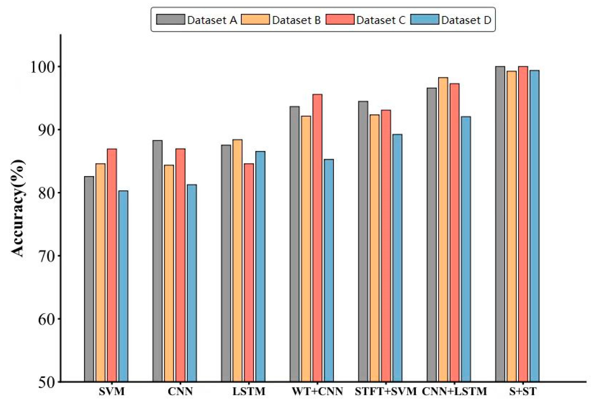
| Diagnostic Methods | Accuracy | |||
|---|---|---|---|---|
| Data A | Data B | Data C | Data D | |
| SVM | 82.56 | 84.58 | 86.93 | 80.29 |
| CNN | 88.27 | 84.35 | 86.95 | 81.26 |
| LSTM | 87.53 | 88.40 | 84.58 | 86.53 |
| WT + CNN | 93.65 | 92.14 | 95.58 | 85.27 |
| STFT + SVM | 94.47 | 92.33 | 93.08 | 89.23 |
| CNN + LSTM | 96.59 | 98.24 | 97.28 | 92.05 |
| S + ST | 100 | 99.25 | 100 | 99.37 |
| CNN | MLP | LSTM | S + ST | |
|---|---|---|---|---|
| 0 db | 88.43 | 65.59 | 87.82 | 100 |
| 2 db | 92.01 | 74.06 | 89.28 | 96.00 |
| 4 db | 93.07 | 79.25 | 93.06 | 98.95 |
| 8 db | 95.02 | 85.06 | 95.35 | 100 |
| Average | 92.1325 | 75.99 | 91.3775 | 98.7375 |
Disclaimer/Publisher’s Note: The statements, opinions and data contained in all publications are solely those of the individual author(s) and contributor(s) and not of MDPI and/or the editor(s). MDPI and/or the editor(s) disclaim responsibility for any injury to people or property resulting from any ideas, methods, instructions or products referred to in the content. |
© 2024 by the authors. Licensee MDPI, Basel, Switzerland. This article is an open access article distributed under the terms and conditions of the Creative Commons Attribution (CC BY) license (https://creativecommons.org/licenses/by/4.0/).
Share and Cite
Yan, J.; Zhu, X.; Wang, X.; Zhang, D. A New Fault Diagnosis Method for Rolling Bearings with the Basis of Swin Transformer and Generalized S Transform. Mathematics 2025, 13, 45. https://doi.org/10.3390/math13010045
Yan J, Zhu X, Wang X, Zhang D. A New Fault Diagnosis Method for Rolling Bearings with the Basis of Swin Transformer and Generalized S Transform. Mathematics. 2025; 13(1):45. https://doi.org/10.3390/math13010045
Chicago/Turabian StyleYan, Jin, Xu Zhu, Xin Wang, and Dapeng Zhang. 2025. "A New Fault Diagnosis Method for Rolling Bearings with the Basis of Swin Transformer and Generalized S Transform" Mathematics 13, no. 1: 45. https://doi.org/10.3390/math13010045
APA StyleYan, J., Zhu, X., Wang, X., & Zhang, D. (2025). A New Fault Diagnosis Method for Rolling Bearings with the Basis of Swin Transformer and Generalized S Transform. Mathematics, 13(1), 45. https://doi.org/10.3390/math13010045