Abstract
Topological structural optimization is a powerful computational tool that enhances the structural efficiency of mechanical components. It achieves this by reducing mass without significantly altering stiffness. This study combines the Natural-Neighbour Radial-Point Interpolation Method (NNRPIM) with a bio-inspired bi-evolutionary bone-remodelling algorithm. This combination enables non-linear topological optimization analyses and achieves solutions with optimal stiffness-to-mass ratios. The NNRPIM discretizes the problem using an unstructured nodal distribution. Background integration points are constructed using the Delaunay triangulation concept. Nodal connectivity is then imposed through the natural neighbour concept. To construct shape functions, radial point interpolators are employed, allowing the shape functions to possess the delta Kronecker property. To evaluate the numerical performance of NNRPIM, its solutions are compared with those obtained using the standard Finite Element Method (FEM). The structural optimization process was applied to a practical example: a vehicle’s suspension control arm. This research is divided into two phases. In the first phase, the optimization algorithm is applied to a standard suspension control arm, and the results are closely evaluated. The findings show that NNRPIM produces topologies with suitable truss connections and a higher number of intermediate densities. Both aspects can enhance the mechanical performance of a hypothetical additively manufactured part. In the second phase, four models based on a solution from the optimized topology algorithm are analyzed. These models incorporate established design principles for material removal commonly used in vehicle suspension control arms. Additionally, the same models, along with a solid reference model, undergo linear static analysis under identical loading conditions used in the optimization process. The structural performance of the generated models is analyzed, and the main differences between the solutions obtained with both numerical techniques are identified.
Keywords:
meshless methods; natural-neighbour radial-point interpolation method; structural optimization; bone remodelling algorithm; evolutionary optimization; automotive industry MSC:
74B10; 74P15
1. Introduction
The past two decades have witnessed a technological revolution, with numerical methods becoming a cornerstone for advancements across various engineering disciplines, and mechanical engineering is no exception. This progress has been further accelerated by the remarkable evolution of computational power observed since the late 20th century. The availability of increasingly fast, efficient, versatile, and practical computational tools has driven the widespread adoption of advanced numerical methods in engineering simulations [1]. In particular, its uses have revolutionized the entire mechanical construction industry, allowing for the design of optimized components based on the manufacturer’s imposed constraints, allowing for a close approximated prediction of the component’s behaviour when subjected to real-life working conditions. In the automotive industry, the structural optimization of various parts is a preponderant factor in the vehicle’s components’ performance and behaviour when subjected to stress throughout the driving procedure, demonstrating promising results in weight reduction while maintaining the necessary resistance to ensure that the component fulfils all its mechanical requirements [2].
In the field of vehicle manufacturing, weight reduction across various components presents an avenue for manufacturers to enhance profitability. Weight reduction often allows for the use of less material per vehicle, further decreasing production costs [3]. By implementing weight reduction strategies and regular optimization processes on the part-design phase, manufacturers can achieve substantial financial gains through these combined effects. In addition to the financial incentive, growing demand and legislative requirements in the automotive industry have created the need to evolve and develop all types of components involved in the various functional sets of a vehicle so that they are lighter, safer, more efficient in relation to production costs, and, specifically for certain components, more comfortable [4]. With the need to meet these requirements, the application of structural optimization methods in the automotive field has grown exponentially over the years, keeping with the improvement and evolution of the computational techniques.
The structural evaluation of automotive components is crucial for the development of efficient and safe parts. One way to perform this is through experimental techniques. For example, Liu et al. [5] developed load spectrum editing for fatigue bench testing, which avoids the need to use the full load spectrum, which could sometimes have minimal impact and significantly increase the testing time. Additionally, computational structural assessment techniques provide engineers with powerful tools to analyse the behaviour of components and systems under various load and stress conditions and complement the overall process of optimization of the studied structure. Through computer simulation, stresses, strains, and displacements can be predicted, allowing the identification of critical failure points to be identified and a efficient optimization of design. For instance, Komurcu et al. [6] took advantage of numerical techniques to tailor the design of a composite suspension control arm to the required manufacturing considerations.
Weight reduction without compromising the structural integrity of the part can be carried out through structural optimization approaches. The suspension control arm has been the object of study combined with structural optimization techniques; for example, Viqaruddin and Ramana Reddy [7] designed a suspension control arm with a 30% weight reduction. Also regarding the same component, Llopis-Albert et al. [8] tested several optimization algorithms to achieve a multiobjective solution for the part. Song et al. [9] had surrogate models, namely the response surface model and the Kriging model, supporting the stuctural optimization of a suspension control arm and achieved weight reduction between 4.13% and 5.22%. Stiffness optimization is also important in addition to the scope of automotive components. For example, Wang et al. [10] used a homogenous stiffness domain index to create an optimization model to improve the stiffness of a machining robot. Finally, optimization approaches are not limited to the optimization of stiffness or weight minimization, along with other aspects such as the friction in bearings [11]. The optimization approach, in this case particle swarm optimization, could also be employed in other applications.
The field of computational mechanics has always been dominated by the use of FEM as the most popular discretization technique in research, development, and education [12]. However, new techniques have been developed to overcome some of the limitations of the FEM related with its rigid mesh dependency. In areas such as fracture and impact mechanics, areas that approach problems that require meshing due to transient domain boundaries, meshless methods have been shown to be a more accurate alternative to FEM due to not being affected by mesh distortion and not requiring meshing. Unlike FEM, in meshless methods, the nodes are distributed in an arbitrary way, and the field functions are approximated based on a domain of influence, rather than an element. In addition, the rule established in FEM that elements cannot overlap does not apply to the domains of influence of meshless methods: they can and should overlap [13].
The first meshless method applied in the context of computational mechanics was the DEM (Diffuse Element Method), developed by Nayroles et al. [14], which used the approximating functions of the Moving Least Squares to construct the approximation functions, a technique previously suggested by Lancaster and S. [15], Dinis et al. [16], Poiate et al. [17]. Later, Belytschko et al. [18] improved the DEM method and developed one of the most popular and widely used meshless methods: the Element Free Galerkin Method (EFGM). Over time, other methods have also been developed, such as the Petrov–Galerkin Local Meshless Method (MLPG) [19], the Finite Point Method (FPM) [20], and the Finite Sphere Method (FSM) [21].
Although these methods have been successfully employed for a variety of issues in the computational mechanics domain, they all present problems and limitations, one of the main ones being the effect of using approximation functions instead of interpolation functions. The PIM (Point Interpolation Method), developed by Liu and Gu [22], proved to be a highly attractive approach, as it effectively solves the challenge of imposing essential boundary conditions by constructing shape functions with the Kronecker’s delta property. Furthermore, PIM simplifies the process of obtaining the derivatives of shape functions. Meanwhile, PIM has evolved with the incorporation of radial basis functions for solving partial differential equations [13,23]. One of the first truly meshless methods to emerge was the NEM (Natural Element Method) [24]. Later, new meshless interpolation methods were proposed, such as PIM (Point Interpolation Method) [22], MFEM (Meshless Finite Element Method) [25], NREM (Natural Radial Element Method) [26], and RPIM (Radial-Point Interpolation Method) [23].
Later, Dinis et al. [16] introduced the Natural-Neighbour Radial-Point Interpolation Method (NNRPIM), a truly meshless method that leverages the connectivity advantages of the Natural Element Method (NEM) and the interpolation capabilities of the Radial-Point Interpolation Method (RPIM). NNRPIM solely relies the on nodal discretization of the problem domain. It then utilizes this spatial information to autonomously distribute integration points and establish nodal connectivity, eliminating the need for a separate background integration mesh as required by EFGM or RPIM [16]. This method differs from RPIM as the connectivity between nodes is not described using domains of influence. Instead, it uses influence cells determined by the Voronoï diagram space decomposer [27] and complemented by the use of Delaunay triangulation [28]. The Voronoï diagram takes on the task of creating the influence cells from a set of unstructured nodes in the domain. The Delaunay triangulation is applied in order to create a background grid with nodal dependence, which is then used in the integration of the interpolation functions of this method. Thus, when compared with a conventional meshless method, NNRPIM can be considered a truly meshless method, since the set of integration points is totally dependent on the nodal distribution [13].
The aim of this study is to utilize a bio-inspired bi-evolutionary optimization algorithm, combined with a natural-neighbour meshless method, for a suspension control arm that has undergone prior accurate modelling and replication. The design of the control arm is based on the geometry of an established industry-standard suspension arm. In automotive mechanical engineering, product development often relies on design philosophies informed by empirical knowledge from engineers. By employing automated techniques to selectively remove material from specific stressed components, it becomes possible to achieve designs that meet manufacturer requirements while significantly reducing mass. Recent literature also highlights a preference for meshless methods, which not only serve as an alternative to FEM but also offer potential advantages [29,30]. Being a truly meshless method possesses some advantages. NNRPIM is capable of discretizing the problem domain using only a nodal distribution. All the other mathematical constructions (nodal connectivity, background integration mesh, shape functions, etc.), required to build the system of equations governing the studied phenomenon, are obtained using only the spatial information of the nodes. In the automotive industry, this feature is an advantage since it allows us to obtain the discretization directly from sketches of CAD software (SOLIDWORKS Student Edition 2023 SP2.1) or the output of 3D scanning. Moreover, as the literature shows, NNRPIM shows a high convergence rate and accuracy, which is convenient in structural optimization algorithms depending on the stress field mapping (as the one used in this work). Accurate predictions of the higher and lower stress levels will lead to better remodelling designs.
2. Natural-Neighbour Radial-Point Interpolation Method
Like any other node-dependent numerical discretization method, NNRPIM discretizes the problem domain with a set of nodes, following a regular or irregular distribution. Then, the Voronoï diagram of the nodal set is constructed, using the mathematical concept of the natural neighbours [31]. For the sake of simplicity, the natural-neighbour procedure will be demonstrated for a 2D Euclidean space, but it can be applied to any n-D space [13]. Considering the set of nodes , discretizing the domain, with . The Voronoï diagram of is the partitioning of the spatial domain discretized by into . Each sub-region is associated with a node so that any point within is closer to than to any other node . The set of Voronoï cells defines the Voronoï diagram, which is . The Voronoï cell can be defined by
Figure 1 depicts the Voronoï diagram for a general nodal discretization. The natural neighbours of node are all the nodes whose Voronoï cells share a common edge with the Voronoï cell of node (represented by the light gray cells surrounding the Voronoï cell of node in Figure 1A). The concept of natural neighbours in NNRPIM replaces the need for a pre-defined connectivity information. The Voronoï diagram automatically generates influence domains (called influence cells in the NNRPIM formulation). With this process, it is possible to define a lower-connectivity influence cell and a higher-connectivity influence cell:
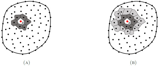
Figure 1.
Nodal connectivity. (A) First-degree influence cell. (B) Second-degree influence cell.
- First-degree influence cells (Figure 1A): These comprise node itself and its immediate natural neighbours. The Voronoï diagram identifies these neighbours as nodes sharing a common edge with the Voronoï cell of .
- Second-degree influence cells (Figure 1B): These encompass node , its first-degree neighbours (including natural neighbours of ), and the natural neighbours of those first-degree neighbours.
After the nodal connectivity is established, it is time to build the grid of background integration points. Thus, in order to integrate the integro-differential equation ruling the physical phenomenon, it is necessary to establish the background integration cells. In NNRPIM, the background integration cells are constructed using only the spatial information of the nodal distribution. This is achieved by applying the Delaunay triangulation numerical technique [13,28], which is product of the Voronoï diagram of the initial nodal distribution [13]. Thus, consider a Voronoï cell of a node , as in Figure 2. It is possible to discretize into smaller quadrilaterals and then apply the Gauss–Legendre quadrature integration scheme to determine the position and weight of integration points within the quadrilaterals. As Figure 2 shows, NNRPIM employs a two-step process to define such integration points. First, each quadrilateral element in a Voronoï cell is transformed into a unit isoparametric square, which allows for the distribution of the integration points within the isoparametric square in compliance with the Gauss–Legendre integration scheme. Then, the isoparametric coordinates are converted back to the actual Cartesian coordinates of the integration. This process is repeated for each Voronoï cell discretizing the problem domain. As suggested in the literature, only one integration point is inserted inside each quadrilateral [13]. Thus, the position of each quadrilateral’s integration point is the quadrilateral’s geometric centre, and its integration weight corresponds to the quadrilateral’s area. A detailed description of the numerical integration procedure of NNRPIM can be found in the literature [13].
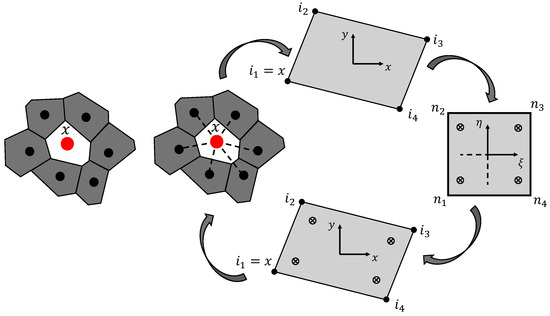
Figure 2.
Adopted NNRPIM procedure for constructing the set of background integration points based on the Voronoï diagram.
Regarding the connectivity of each integration point, integration points located within the Voronoï cell inherit the nodal connectivity of node (i.e., inherit its influence cell). In the NNRPIM, nodal connectivity arises naturally from the overlap of influence cells associated with each integration point. These influence cells define the set of nodes contributing to the shape function construction and stiffness matrix assembly [13].
The next step is the construction of the shape functions. The NNRPIM uses the radial point interpolators (RPI) technique, which allows the interpolation of the variable field at an integration point . Thus, consider a function , defined in the domain , discretized by a set of nodes , and assuming that only the nodes included in the influence domain of the point of interest have an effect on . The value of the function at the point can be obtained from the following expression:
in where represents a radial basis function, n is the number of nodes inside the influence cell of , and and are non-constant coefficients of and , respectively.
Several radial basis functions can be used, and several have been studied and developed over the years. In this work, as recommended in the literature [13], the multiquadratic radial basis function (MQ-RBF) function will be used [32]. The MQ-RBF can be described as follows:
for which is defined as
The variable is the integration weight of integration point , and c and p are MQ-RBF shape parameters. In the literature, it is possible to find works studying the influence of the MQ-RBF shape parameters on the constructed shape functions [13]. It was found that assuming and leads to shape functions with the delta Kronecker [13]. Thus, these are the values used in this work. In order to guarantee a unique solution [23], the following system of equations is added:
Assuming a linear polynomial basis , with , it is possible to present Equation (2) as
solving this system of equations allows us to define the non-constant coefficients and ,
Inserting and into Equation (2), the following interpolation is obtained:
And, finally, the RPI shape function is defined,
In elasto-static problems, the equilibrium equations governing the partial differential equilibrium can be summarized as: , in which represents the gradient vector, the Cauchy stress tensor, and the body force vector. Regarding the boundary surface, it can be divided into two types: natural boundaries (), where , and essential boundaries (), where . The imposed displacement at the essential boundary is represented as , and the traction force on the natural boundary is defined by (where is a unit vector normal to the natural boundary ).
The Cauchy stress tensor can be represented in Voigt notation, , as well as the strain tensor, . Applying Hooke’s law, it is possible to relate the stress state with the strain state, , being the strain obtained from the displacement field: . For a generic 3D problem, the differential operator matrix L and the material constitutive matrix c can be represented as
where and . To establish the system of equations, the virtual work principle is assumed, and energy conservation is imposed:
With the simplification of the above expression, the following can be obtained:
which results in the simplified expression , where represents the global stiffness matrix, which can be numerically calculated with:
The matrix, known as the deformability matrix, can be defined as
With Equation (12), the body force () and external force vectors () can also be defined:
where represents the weight of the integration point on the surface where the external force is being applied, is the number of integration points defining the boundary where the force is applied, and is the interpolation matrix.
The essential boundary conditions are imposed directly on the stiffness matrix , since RPI shape functions possess the Kronecker delta property. If the problem can be analysed assuming a plane stress simplification, the problem reduces to a 2D analysis, and all components associated with the direction are removed, thus, reducing the size of all algebraic structures previously presented. For instance, the constitutive matrix and the stress and strain vectors become
and the deformability and interpolation matrices are reduced to
3. Structural Topology Optimization
In computational mechanics, topological optimization is one of the most studied types of optimization due to its ability to generate more efficient and innovative designs. A topological optimization involves the strategic redistribution of material in a structure, resulting in shapes and geometries that are optimized to meet specific criteria, such as strength, stiffness, or other mechanical performance criteria. Assuming a standard topological optimization problem for a given structure, where the aim is to achieve a layout that is as rigid as possible while constraining the structure’s mass, the problem can be formulated by minimizing the average compliance, with the material’s weight constrained. The problem may be described as follows:
where C represents the average compliance of the structure, the mass of the selected structure, and the mass of node i. The design variable indicates the presence ( or absence ( of a node in the layout of the defined domain.
Evolutionary computation is a search technique inspired by biological evolution, which uses selection, reproduction and variation to find optimized solutions to complex problems [33]. In relation to the more conventional optimization techniques, evolutionary techniques are more robust, exploratory and flexible, making them ideal for complex problems with challenging cost functions. Methods such as ESO (Evolutionary Structural Optimization), developed by Xie and Steven [34], have been widely applied to structural optimization problems in recent years [34]. The technique is based on the removal of material from a specific domain through an iterative process, material that is considered inefficient and redundant, in order to obtain a design that is considered optimal [35]. Despite the widespread use of the ESO method, this method presents problems and limitations that have led to the necessity of investigating new techniques. In order to improve the viability of the solutions obtained in the optimization, the need to create a bidirectional algorithm appears, which would allow not only the removal of material in order to eliminate areas that demonstrated low stress but also the addition of material to compensate for areas of high stress. This led to the creation of the bidirectional evolutionary structural optimization method, or BESO (Bi-Directional Evolutionary Structural Optimization), a method inspired not only by the material removal capabilities of ESO but also by the additive material capabilities of AESO [36], an additive evolutionary structural optimization method (Addition Evolutionary Structural Optimization), which allows for a more careful search of the design domain while also offering a superior ability to find the global minimum [37].
An elasto-static analysis step initiates each optimization iteration, returning the displacement, strain, and stress fields. As such, it is possible to calculate the equivalent von Mises stress for each integration point, as well as the cubic average of the von Mises stress field, which serves as a reference to help detecti sudden stress changes. With a high value of stress, the cubic average is highly affected. Meanwhile, with low values of stress, the average is practically unaltered.
Next, a penalty system is applied in order to describe and attribute a specific parameter, in this specific case the density, to each integration point. In this work, the interval values for the penalty are assumed to be , where 1 represents the rewarded domains, or solid material, and the penalized domain, or removed material. The BESO procedure performance depends on the reward ratio, , and the penalization ratio, . The integration points with the highest and the integration points with the lowest are identified. The points are rewarded with , while the points are penalized with . Each node is then assigned a penalty parameter . For each integration point , the closest nodes update their penalty values with . After updating all nodes, the penalty parameters for each integration point are recalculated in order to filter and smooth the selected penalty parameters using the interpolation function , where n is the number of nodes inside the analyzed influence domain of , and is the shape function vector of the integration point . At the end of the first iteration, some values differ from one, indicating the absence of material. The process can then proceed to the next iteration. In iteration j, the penalty parameters will be used to modify the material constitutive matrix. Consequently, the penalized constitutive material matrix is calculated. In the following iteration j, the stiffness matrix is calculated, using instead of . The same steps follow, and a new equivalent von Mises stress field is obtained. Through it, the new cubic average stress is calculated, and the comparison is made. If the condition is true, the integration points with are rewarded with . The penalty parameters are recalculated, updating the material domain for the next iteration .
The structural optimization algorithm used in the present work is a BESO - inspired algorithm, developed for applications in the biomechanics field, namely bone-remodelling applications. In a relation known as Wolff’s law, bone tissue directionality increases its stiffness in response to external applied loads [38]. In order to predict this behaviour, several researchers have developed laws based on observations and experimental tests able to predict bone behaviour based on the different load cases considered. The created models are the basis for computational bone analysis, and the model used affects the results of the simulations carried out. Various models have been established, ranging from the Pauwels’ model [39] to other models with extra considerations or different approaches to the problem, such as the Corwin’s [40] and Carter’s [41].
Carter’s model is identical to Pauwels’ model in that it requires a mechanical stimulus for remodelling to occur. This stimulus is calculated based on the effective stress, which takes into account both the local stress and the bone density, as well as the number of load cycles to which the bone is subjected (represented by the exponent k). The higher the magnitude of stress, the stronger the stimulus for remodelling.
The model assumes that the applied stress acts as a built-in optimization tool. The goal is to achieve a balance between maximizing the structural integrity of the bone (strength) and minimizing its mass. This can be achieved by minimizing an objective function that mathematically represents this goal.
The model also offers the option of using stress or strain energy as the basis for optimization. Strain energy focuses on maximizing the bone’s stiffness (resistance to bending), while stress focuses on optimizing the material’s strength. By using strain energy, the model relates the apparent density of the bone to the local strain energy it experiences. This makes it possible to estimate the bone’s density at the remodelling equilibrium, a state in which bone resorption and formation are balanced.
If the bone is under stress from several directions, the model combines the effects of each stress pattern in a single direction. This direction is referred to as the normal vector () and represents the ideal alignment for the bone’s internal support structures (trabeculae) for optimum strength. To calculate this ideal direction, the model considers the normal stress acting on the entire bone, which is specified in Equation (27).
The algorithm, originally developed for this work, was incorporated in the previous codes already programmed by the research team, which included a bone-remodelling model adapted for meshless methods developed by Belinha et al. [42]. This new approach assumes that a mechanical stimulus, adequately represented by stress and potentially strain metrics, serves as the key factor influencing the bone-tissue-remodelling process. A detailed description of the entire model can be found in the literature [13]. Through the described bone-remodelling procedure, the remodelling itself functions as a topological optimization algorithm. Thus, in each iteration, only the points with high/low values of energy deformation density optimize the density based on its mechanical stimulus. A detailed description of the procedure can be found in the literature [13]. Figure 3 presents a scheme of how the optimization topology algorithm inspired by the bone-remodelling flowchart would present the NNRPIM method. As the flowchart shows, the structural optimization algorithm applied in this work is iterative. Thus, in each iteration, for a given material distribution, the stiffness matrix is calculated and the variable fields are obtained (displacements, strains, and stresses). Then, the integration points with lower stress levels have their material density reduced, which will reduce their mechanical properties (notice that is the total number of integration points and is the penalization ratio, established in the beginning of the analysis). A similar procedure occurs for the integration points a with a higher stress level; their material density will increase, which will increase their mechanical properties (where is the reward ratio, established at the beginning of the analysis). Then, in the next iteration, the material distribution changes, leading to new variable fields and a consequent new remodelling scenario. The remodelling process ends when the average density of the model is lower than a threshold valued initially defined by the user. Since the FEM and NNRPIM formulations are different (from a mathematical point of view), for the same material model, they lead to different variable fields (very close, but different). Because the adopted optimization algorithm is iterative, and since the solution of the next iteration is dependent on the solution of the previous iteration, it is not straightforward that the FEM and NNRPIM analyses tend to the same solution.
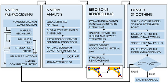
Figure 3.
Flowchart of the topology optimization algorithm combined with the NNRPIM.
4. Numerical Results
This section presents the numerical results obtained in the optimization study of a vehicle’s control arm; a comparison of the results obtained with NNRPIM, which involves the implementation of the numerical methodology presented previously; and FEM. For all numerical simulations, the dimensional approach to the numerical analysis was for plane stress, so the stress vector normal to the plane is equal to zero. In this work, the following formulations were used to perform the optimization analyses:
- FEM: three-node 2D linear triangular elements with constant strain;
- NNRPIM: second-degree influence cells, MQ-RBF shape parameters and , constant polynomial basis, and integration points per quadrilateral integration sub-cell.
4.1. Control Arm Optimization
In this subsection, the proposed optimization numerical technique is used to optimize the stiffness of a standard suspension control arm using the FEM and the NNRPIM as solvers. The BESO algorithm is inspired in a bone-remodelling model, allowing as output nonbinary density distributions. This approach avoids chess pattern solutions.
The parameters associated with the optimization algorithm were selected based on the literature [43,44]. The literature shows that that as the nodal mesh becomes denser, the solution becomes more complex, with more trusses and more micro-trusses [43,44]. Additionally, the solution complexity is also related to the penalization and reward ratios. For instance, a very dense nodal mesh assuming a large penalization ratio will lead to simpler solutions (lower number of trusses and almost no micro-trusses); at the same time, this solution will be very well defined (with the contours of the trusses being well defined). It was found that, for the nodal mesh density considered in this paper, the best penalization ratio is about 2% and 5% [43,44]. However, for denser meshes, a penalization ratio of 10% is also admissible. Thus, taking into consideration the nodal mesh density of the models analyzed in this work, penalization ratios of 5% and 10% will be considered, and the reward ratio will be kept at .
The effective von Mises stress criterion will be used exclusively. The working procedure consisted of searching for a three-dimensional CAD model of a relatively functional component, where its geometry would be simplified to a two-dimensional format in Solidworks® Student Edition 2023 SP2.1 (Figure 4). Subsequently, the 2D sketch created was exported to FEMAP 2021.2 MP1 (student version), where its mesh was created and then imported into the code written by the authors.
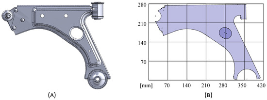
Figure 4.
Standard suspension control arm models: (A) 3D CAD and (B) 2D CAD.
Four meshes were built, corresponding to four different case studies that will be analysed: a mesh without the arm’s characteristic perforation, a mesh with the perforation, and the respective versions created by dividing sections of the arm to avoid reducing the density of the material in the areas with applied boundary conditions (Figure 5).
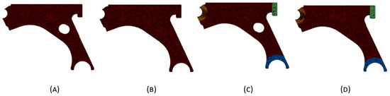
Figure 5.
Adopted nodal discretizations of the solid domain. (A) Model D1—discretization with central perforation. (B) Model D2—discretization of the solid model without perforation. (C) Model D3—discretization of the model with central perforation, assuming remodelling domain constraints. (D) Model D4—discretization of the solid model (without perforation) with remodelling domain constraints.
The purely academic material properties considered were as follows: Young’s modulus E = 1 MPa and Poisson’s ratio = 0.3. Since the variable fields (displacement, strain, and stress fields) are obtained assuming a material linear-elastic behaviour, and only small strains are considered, the stress field does not depend on the Young’s modulus. Thus, the solution obtained using these purely academic material properties is equal to the solution obtained with any other positive Young’s modulus value. The essential and natural boundary conditions presented in Figure 6 were assumed, allowing us to simulate the displacement constrains and external loads of the control arm. At the circular surface, a distributed load of N/mm was applied. The described boundary conditions simulate bending (flexion) of the analysed component, a common mechanical behaviour experienced during its operation.
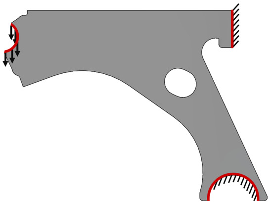
Figure 6.
Schematic representation of the natural and essential boundary conditions considered.
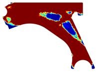
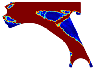
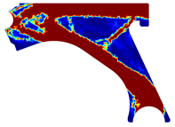
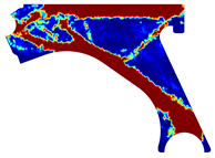
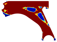
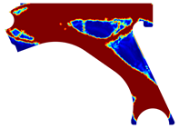
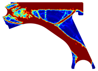
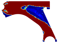
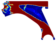
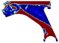
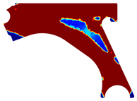
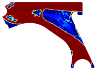
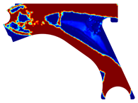
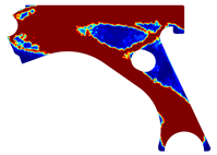
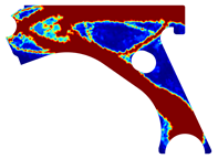
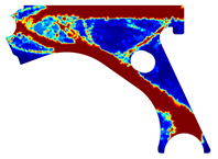
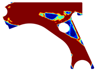
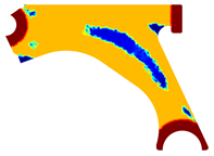
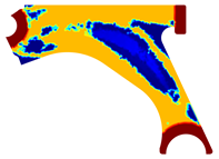
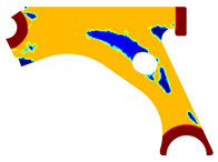
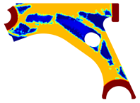
The obtained topologies for the different meshes and control arm arrangements considered are presented in Table 1, Table 2, Table 3 and Table 4. In each one of these tables, is possible to find the FEM and NNRPIM results, obtained at distinct iterations. Thus, in the first two lines of the tables, the FEM and NNRPIM results obtained for a penalization ratio of are presented. Notice that the mass obtained for each iteration () decreases as the remodelling procedure evolves and the iteration increases. In the last two lines of the tables, the results obtained for both FEM and NNRPIM (considering ) are shown. The colormap of the figures included in the tables corresponds to the volume fraction distribution and follows the corresponding colorbar shown in each table.

Table 1.
Material remodelling solutions obtained with the discretized model D1. For each analysis, four iterations are represented, and the iteration number and corresponding mass (with respect to the initial mass ) are presented.
Table 2.
Material remodelling solutions obtained with the discretized model D2. For each analysis, four iterations are represented, and the iteration number and corresponding mass (with respect to the initial mass ) are presented.
Table 3.
Material remodelling solutions obtained with the discretized model D3. For each analysis, four iterations are represented, and the iteration number and corresponding mass (with respect to the initial mass ) are presented.
Table 4.
Material remodelling solutions obtained with the discretized model D4. For each analysis, four iterations are represented, and the iteration number and corresponding mass (with respect to the initial mass ) are presented.
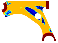
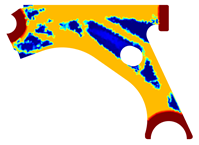
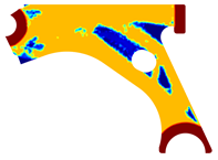
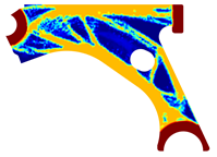
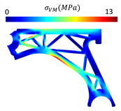
Recalling the flowchart in Figure 3, in each iteration using FEM or NNRPIM, the displacement field is obtained; then, the strain and stress fields are calculated, and the von Mises stress field is defined. With the von Mises stress field, it is possible to decide which material points (integration points) will be remodelled. Thus, integration points (with lower stress levels) will reduce their volume fraction (and consequently their mechanical properties), and integration points (with higher stress levels) will increase their volume fraction and mechanical properties. Atthe end of each iteration, based in this information, the volume fraction of each material point is actualized, leading to a transient material map. In Table 1, Table 2, Table 3 and Table 4, it is possible to visualize the modification of the material map, where the results of only four iterations (three intermediary interesting iterations and the last iteration of the analysis) are presented.
The analysis of the design solutions revealed that the perforation in the control arm corresponds to a null stress zone. Situated in the primary zone of material removal, this perforation serves solely to reduce the component’s overall mass. Therefore, the perforation has no impact on the mechanism’s functionality. The solutions obtained reflect that there is the possibility of more drastic material removal in relation to the original removal. The obtained topologies reveal highly binary structures (topologies) across the entire density field. It is possible to observe that yielded the most successful solutions. These solutions showcased a clear improvement and connection between generated sections, particularly evident in the initial and final iterations of the NNRPIM method. A difference between the FEM and NNRPIM solutions was observed in the final iteration volume fraction.
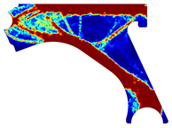
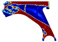
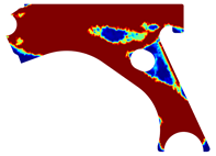
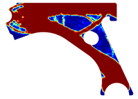
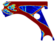
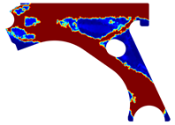
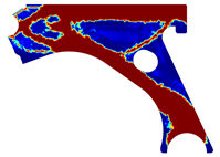
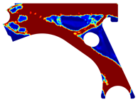
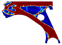
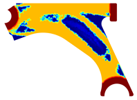
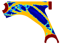
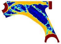
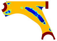
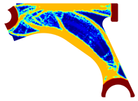
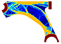
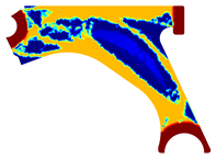
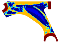
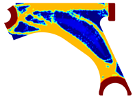
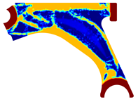
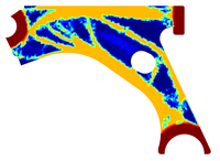
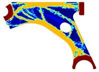
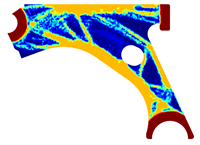
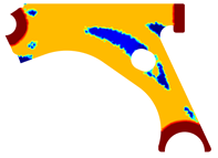
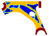
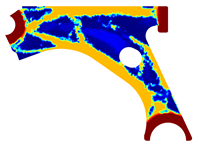
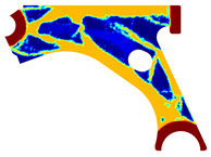
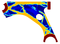
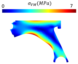
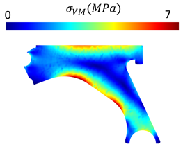
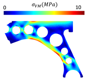
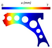
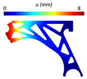
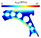
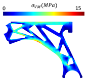
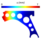
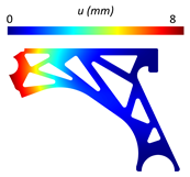
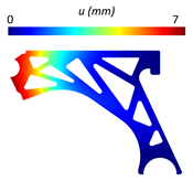
For a more practical and direct comparison, two solutions from each method (FEM and NNRPIM) were separated from Table 4. Figure 7 shows two solutions of the previously presented optimization of the control arm (corresponding to the model with no inside perforation) with density reduction restriction in the boundary condition zone, for . The iteration chosen to analyse the final result of the algorithm used was the very last one.
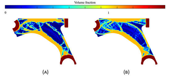
Figure 7.
Remodelling material solutions obtained at iteration 30, with discretization D4 (assuming a density reduction restriction in the boundary conditions sections), for with (A) the FEM method and (B) the NNRPIM method.
Visually, the superior truss connection and the creation of a greater number of intermediate densities in the NNRPIM are noticeable. Both these aspects would be potentially important factors in additive manufacturing production, since they are both prevalent to the component’s structural performance.
4.2. Topology Design and Structural Analysis
Three models based on the previously obtained optimized solutions were built Figure 8A,C,D. These three models do not resemble the designs used in the automotive industry, which prefers designs with less sharp angles in the inner voids to reduce local stress concentrations. Generally, the industrial automotive solutions include circular holes, which are able to reduce the stress concentration phenomenon [45]. Therefore, a commonly used design for the control arm was considered as well, as Figure 8B shows. Model 1 is inspired ny the solutions assuming a central perforation (Table 4). Model 3 is a reinforced version of the solutions suggested in Table 3. Model 4 is based on model 3 with a modified boundary contour. The thickness of the boundary contour is increased by 50% (1.5 times the nominal thickness) relatively to the baseline model, using a 6 mm offset in relation to the outer delineation of the model.
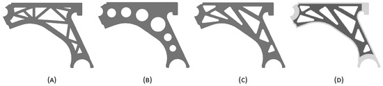
Figure 8.
Constructed models for the linear elasticity analysis. (A) Model 1, (B) Model 2, (C) Model 3 and (D) Model 4.
Then, to each model of Figure 8, the essential and natural boundary conditions described in Figure 6 were imposed and static linear analyses were performed.
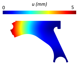
Table 5 provides the displacement and von Mises stress distributions calculated using FEM and NNRPIM for the fully solid model. A comparison of the two methods shows reduced differences in the displacement and von Mises effective stress fields.
Table 5.
Variable fields of interest (displacement and von Mises stress) obtained for the solid control arm.
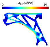
It is possible to observe that model 2 demonstrated the best mechanical performance, justified by the lower von Mises stress and higher stiffness than the other models designed and an even higher specific stiffness than the solid arm. These results support initial expectations, as the removal of material in a circular shape allows for a more uniform distribution of stresses in the structure. As a result, the stress is not concentrated at specific points, which leads to a reduction in the risk of structural failure and an increase in the overall stiffness of the part.
Triangular material removal leaves behind a pattern resembling interconnected triangles. This process effectively creates a truss-like structure that is more efficient in transferring loads, as well as easier to manufacture. Regarding the behaviour of models 1, 3 and 4, based on triangular material removal, model 4 presented the higher stiffness. However, this stiffness is due to the increased thickness of the outside struts, which has an effect on specific thickness as it increases less than models 1 and 3. Between model 1 and 3, the specific stiffnesses are equal. However, a distinction between both can be made regarding the smoothness of the obtained stress fields. It can be seen in Table 6 and Table 7 that the stresses are only slightly better distributed in Model 3, which presents a lower peak von Mises stress.
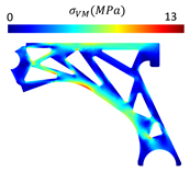
Table 6.
Obtained variable fields of interest (displacements and von Mises stresses) with FEM, for each of the four analysed models.
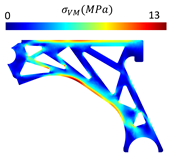
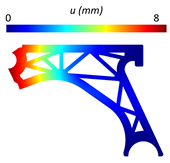
Table 7.
Obtained interest variable fields (displacements and von Mises stresses) with NNRPIM, for each of the four analysed models.
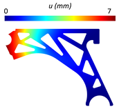
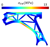
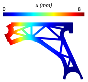
The displacement and von Mises stress fields are shown in Table 6 and Table 7 for the FEM and NNRPIM, respectively. Comparing both tables, the two methods present very similar solutions. Recall that the objective function of the adopted optimization procedure, Equation (3), aims to reduce the mass and at the same time maximize the stiffness of the mechanical component (by the minimization of the structural compliance). Therefore, in Table 8, the mass and directional stiffness of each model are calculated with the results obtained with both methods. The directional stiffness K is calculated with
where n is the number of nodes along the natural neighbour, is the force applied at node of the natural boundary in direction , and is the displacement obtained at the same node in the same direction .
Table 8.
Results obtained with the model of the solid structure and with the proposed designed models M1 to M4.
Compared to FEM analysis, the NNRPIM solutions obtained for models 2, 3, and 4 exhibited higher maximum von Mises stress values. Similarly, FEM displayed slightly lower displacements compared to NNRPIM, suggesting a stiffer solution. The FEM formulation used is the constant-strain triangular element, and the literature shows that this formulation produces stiffer results for bending problems (such as the one analysed in this work) [46]. Nonetheless, both these discrepancies are very small, allowing us to conclude that both techniques produce similar results.
Finally, both methods are quantitatively compared in Table 9, which shows the relative difference between the interest metrics calculated through the FEM and NNRPIM. The relative difference between methodologies is calculated by
where is the variable value obtained with NNRPIM and is the same variable value obtained by FEM. Table 9 shows that the relative differences between both methods are very reduced. Regarding the displacement, the relative difference is generally about , being even lower in model 1 (). Concerning the maximum von Mises stress, the relative difference shows more variation, being low for the solid model and higher for models 2, 3 and 4. For the relative difference of the directional stiffness, it is interesting to observe that FEM and NNRPIM produce similar results, and that the relative difference between all the other models is very low (between and ).
Table 9.
Relative difference between the critical variables calculated through FEM or NNRPIM.
5. Conclusions
The focus of this work was the application of the NNRPIM, combined with a bi-evolutionary topological optimization algorithm, for the analysis of a standard automotive mechanical component. In parallel, a well-known FEM formulation was also used for comparison purposes. The analysed mechanical component was a standard suspension control arm, in which the 3D CAD was converted to a simplified two-dimensional layout in order to streamline and minimize the computational cost of the numerical simulations conducted.
When assessing the obtained solutions, it was noticeable that NNRPIM generated topologies with better truss connection and a higher number of intermediate densities (intricate bone-like trabecular distributions), features that would greatly benefit the mechanical performance of an hypothetical part manufactured by means of additive manufacturing. Subsequently, four designs were built based on a solution obtained from the previously mentioned algorithm, following material-removal approaches commonly applied in the automotive industry for the studied component: a model with a trussed design, a model with circular material removal, a model with triangular material removal, and a model equivalent to the previously mentioned, albeit with an increase in the boundary contour thickness to 1.5 times the nominal thickness of the remaining model. By means of an linear static analysis in the same conditions applied to the optimization algorithm, it was observable that the design based on circular material removal demonstrated the best stiffness and specific stiffness, proving the original hypothesis, since the circular shape allows for a more uniform distribution of stresses in the structure. This kind of solution is recurrent in the automotive industry, and the results presented show that this simple solution is efficient and practical. The trussed and triangular models exhibited similar behaviour, as the principle for their material removal is similar. Model 4 (reinforced at the contour), as expected, displayed a lower displacement, and consequently a higher stiffness, compared to model 3. However, as a result, its increase in mass and total volume led to a negligible difference in specific stiffness between models 3 and 4. There were minor discrepancies observed in the von Mises stress fields and maximum stress values obtained with FEM and NNRPIM. Similarly, small differences were observed in the displacement values, which can be attributed to the higher rigidity of triangular elements.
Regarding the relative difference between both formulations, the obtained results show that concerning the displacement, NNRPIM is able to produce results very close to FEM. For instance, for model 1, the relative difference is , and for all the other models, the relative difference ranges between and . Regarding the maximum von Mises stress, the results show that the relative differences obtained for the solid model and model 1 are and , respectively, which are very close. However, for models 2, 3 and 4, the relative difference increases, ranging from and , indicating that some stress-concentration zones produce distinct von Mises stress values. The directional stiffness of both formulations is very close, ranging between and . These results reinforce the idea that NNRPIM is a valid numerical alternative to the FEM.
In other applications associated with remodelling and BESO algorithms, NNRPIM already proved to be efficient, delivering optimal solutions for automotive parts, such as wheels and brake pedals [44], or the development of new optimized functional materials [47] and their cellular foam structure [48]. In this work, it was shown again that NNRPIM is able to produce results with satisfactory similarity to FEM, indicating that it could represent a viable alternative to FEM topological optimization analyses. Future research directions on this topic will include the extension of the application to 3D analyses in order to include out-of-plane forces and torsion effects; the inclusion of functionally foam material (to fill the voids and reduce stress concentration phenomena) and its prototype production and experimental validation using 3D printing techniques; and the inclusion of artificial neural networks to surrogate the FEM/NNRPIM processing block, allowing for much faster computational analysis [49].
Author Contributions
Conceptualization, J.B. and A.P.; methodology, J.B. and A.P.; software, J.B. and A.P.; validation, J.B., C.O. and A.P.; formal analysis, J.B., C.O. and A.P.; investigation, J.B., C.O. and A.P.; resources, J.B. and A.P.; data curation, J.B., A.P. and C.O.; writing—original draft preparation, C.O.; writing—review and editing, J.B. and A.P.; visualization, J.B. and A.P.; supervision, J.B.; project administration, J.B.; funding acquisition, J.B. All authors have read and agreed to the published version of the manuscript.
Funding
This research received no external funding.
Institutional Review Board Statement
Not applicable.
Informed Consent Statement
Not applicable.
Data Availability Statement
The original contributions presented in the study are included in the article, further inquiries can be directed to the corresponding author.
Conflicts of Interest
The authors declare no conflicts of interest.
References
- Oanta, E.; Raicu, A.; Menabil, B. Applications of the numerical methods in mechanical engineering experimental studies. IOP Conf. Ser. Mater. Sci. Eng. 2020, 916, 012074. [Google Scholar] [CrossRef]
- Jones, D. Optimization in the Automotive Industry. In Optimization and Industry: New Frontiers; Springer: Boston, MA, USA, 2003. [Google Scholar] [CrossRef]
- Witik, R.; Payet, J.; Michaud, V.; Ludwig, C.; Månson, J. Assessing the life cycle costs and environmental performance of lightweight materials in automobile applications. Compos. Part A Appl. Sci. Manuf. 2011, 42, 1694–1709. [Google Scholar] [CrossRef]
- Matsimbi, M.; Nziu, P.K.; Masu, L.M.; Maringa, M. Topology Optimization of Automotive Body Structures: A review. Int. J. Eng. Res. Technol. 2021, 13, 4282–4296. [Google Scholar]
- Liu, X.; Tan, J.; Long, S. Multi-axis fatigue load spectrum editing for automotive components using generalized S-transform. Int. J. Fatigue 2024, 188, 108503. [Google Scholar] [CrossRef]
- Komurcu, E.; Kefal, A.; Abdollahzadeh, M.; Basoglu, M.; Kisa, E.; Yildiz, M. Towards composite suspension control arm: Conceptual design, structural analysis, laminate optimization, manufacturing, and experimental testing. Compos. Struct. 2024, 327, 117704. [Google Scholar] [CrossRef]
- Viqaruddin, M.; Ramana Reddy, D. Structural optimization of control arm for weight reduction and improved performance. Mater. Today Proc. 2017, 4, 9230–9236. [Google Scholar] [CrossRef]
- Llopis-Albert, C.; Rubio, F.; Zeng, S. Multiobjective optimization framework for designing a vehicle suspension system. A comparison of optimization algorithms. Adv. Eng. Softw. 2023, 176, 103375. [Google Scholar] [CrossRef]
- Song, X.G.; Jung, J.H.; Son, H.J.; Park, J.H.; Lee, K.H.; Park, Y.C. Metamodel-based optimization of a control arm considering strength and durability performance. Comput. Math. Appl. 2010, 60, 976–980. [Google Scholar] [CrossRef]
- Wang, Z.; Gao, D.; Deng, K.; Lu, Y.; Ma, S.; Zhao, J. Robot base position and spacecraft cabin angle optimization via homogeneous stiffness domain index with nonlinear stiffness characteristics. Robot. Comput.-Integr. Manuf. 2024, 90, 102793. [Google Scholar] [CrossRef]
- Shi, J.; Zhao, B.; He, J.; Lu, X. The optimization design for the journal-thrust couple bearing surface texture based on particle swarm algorithm. Tribol. Int. 2024, 198, 109874. [Google Scholar] [CrossRef]
- Rao, S. The Finite Element Method in Engineering, 6th ed.; Butterworth-Heinemann: Oxford, UK, 2018. [Google Scholar] [CrossRef]
- Belinha, J. Meshless Methods in Biomechanics—Bone Tissue Remodelling Analysis; Springer International: Berlin/Heidelberg, Germany, 2014; Volume 16. [Google Scholar] [CrossRef]
- Nayroles, B.; Touzot, G.; Villon, P. Generalizing the finite element method: Diffuse approximation and diffuse elements. Comput. Mech. 1992, 10, 307–318. [Google Scholar] [CrossRef]
- Lancaster, P.; Salkauskas, K. Surfaces generated by moving least squares methods. Math. Comput. 1981, 37, 141–158. [Google Scholar] [CrossRef]
- Dinis, L.; Natal Jorge, R.; Belinha, J. Analysis of 3D solids using the natural neighbour radial point interpolation method. Comput. Methods Appl. Mech. Eng. 2007, 196, 2009–2028. [Google Scholar] [CrossRef]
- Poiate, I.; Vasconcellos, A.; Mori, M.; Poiate, E. 2D and 3D finite element analysis of central incisor generated by computerized tomography. Comput. Methods Programs Biomed. 2011, 104, 292–299. [Google Scholar] [CrossRef]
- Belytschko, T.; Lu, Y.; Gu, L. Element-free Galerkin methods. Int. J. Numer. Methods Eng. 1994, 37, 229–256. [Google Scholar] [CrossRef]
- Atluri, S.; Zhu, T. A new meshless local Petrov–Galerkin (MLPG) approach. Comput. Mech. 1998, 22, 117–127. [Google Scholar] [CrossRef]
- Oñate, E.; Idelsohn, S.; Zienkiewicz, O.; Taylor, R. A finite point method in computational mechanics. Applications to convective transport and fluid flow. Int. J. Numer. Methods Eng. 1996, 39, 3839–3866. [Google Scholar] [CrossRef]
- De, S.; Bathe, K. Towards an efficient meshless computational technique: The method of finite spheres. Int. J. Numer. Methods Eng. 2001, 170, 3839–3866. [Google Scholar] [CrossRef]
- Liu, G.; Gu, Y. A point interpolation method for two-dimensional solid. Int. J. Numer. Methods Eng. 2001, 50, 937–951. [Google Scholar] [CrossRef]
- Wang, J.; Liu, G. A point interpolation meshless method based on radial basis functions. Int. J. Numer. Methods Eng. 2002, 54, 1623–1648. [Google Scholar] [CrossRef]
- Sukumar, N.; Moran, B.; Belytschko, T. The Natural Element Method in Solid Mechanics. Int. J. Numer. Methods Eng. 1998, 43, 839–887. [Google Scholar] [CrossRef]
- Idelsohn, S.; Oñate, E.; Calvo, N.; Del Pin, F. Meshless finite element method. Int. J. Numer. Methods Eng. 2003, 58, 893–912. [Google Scholar] [CrossRef]
- Belinha, J.; Dinis, L.; Natal Jorge, R. The natural radial element method. Int. J. Numer. Methods Eng. 2013, 93, 1286–1313. [Google Scholar] [CrossRef]
- Voronoï, G. Nouvelles applications des paramètres continus à la théorie des formes quadratiques. Deuxième mémoire. Recherches sur les parallélloèdres primitifs. J. Für Die Reine Und Angew. Math. 1908, 134, 198–287. [Google Scholar] [CrossRef]
- Ito, Y. Delaunay Triangulation. In Encyclopedia of Applied and Computational Mathematics; Engquist, B., Ed.; Springer: Berlin/Heidelberg, Germany, 2015; pp. 332–334. [Google Scholar] [CrossRef]
- Juan, Z.; Shuyao, L.; Yuanbo, X.; Guangyao, L. A Topology Optimization Design for the Continuum Structure Based on the Meshless Numerical Technique. Comput. Model. Eng. Sci. 2008, 34, 137–154. [Google Scholar] [CrossRef]
- Zou, W.; Zhou, J.; Zhang, Z.; Li, Q. A Truly Meshless Method based on Partition of Unity Quadrature for Shape Optimization of Continua. Comput. Mech. 2007, 39, 357–365. [Google Scholar] [CrossRef]
- Sibson, R. A brief description of natural neighbour interpolation. In Interpreting Multivariate Data; John Wiley & Sons: Hoboken, NJ, USA, 1981; pp. 21–36. [Google Scholar]
- Hardy, R. Theory and applications of the multiquadric-biharmonic method 20 years of discovery 1968–1988. Comput. Math. Appl. 1990, 19, 163–208. [Google Scholar] [CrossRef]
- Bendsøe, M.; Sigmund, O. Topology Optimization. Theory, Methods, and Applications, 2nd ed.; Corrected Printing; Springer International: Berlin/Heidelberg, Germany, 2004. [Google Scholar] [CrossRef]
- Xie, Y.; Steven, G.P. Optimal design of multiple load case structures using an evolutionary procedure. Eng. Comput. 1994, 11, 295–302. [Google Scholar] [CrossRef]
- Abolbashari, M.; Keshavarzmanesh, S. On various aspects of application of the evolutionary structural optimization method for 2D and 3D continuum structures. Finite Elem. Anal. Des. 2006, 42, 478–491. [Google Scholar] [CrossRef]
- Querin, O.; Steven, G.; Xie, Y. Evolutionary structural optimisation using an additive algorithm. Finite Elem. Anal. Des. 2000, 34, 291–308. [Google Scholar] [CrossRef]
- Querin, O.; Young, V.; Steven, G.; Xie, Y. Computational efficiency and validation of bi-directional evolutionary structural optimisation. Comput. Methods Appl. Mech. Eng. 2000, 189, 559–573. [Google Scholar] [CrossRef]
- Fuchs, R.; Warden, S.; Turner, C. 2—Bone anatomy, physiology and adaptation to mechanical loading. In Bone Repair Biomaterials; Planell, J.A., Best, S.M., Lacroix, D., Merolli, A., Eds.; Woodhead Publishing Series in Biomaterials; Woodhead Publishing: Sawston, UK, 2009; pp. 25–68. [Google Scholar] [CrossRef]
- Pauwels, F. Gesammelte Abhandlungen zur Funktionellen Anatomie des Bewegungsapparates; Springer: Berlin/Heidelberg, Germany, 1965. [Google Scholar] [CrossRef]
- Cowin, S. The relationship between the elasticity tensor and the fabric tensor. Mech. Mater. 1985, 4, 137–147. [Google Scholar] [CrossRef]
- Carter, D.; Fyhrie, D.; Whalen, R. Trabecular bone density and loading history: Regulation of connective tissue biology by mechanical energy. J. Biomech. 1987, 20, 785–794. [Google Scholar] [CrossRef] [PubMed]
- Belinha, J.; Natal Jorge, R.; Dinis, L. A meshless microscale bone tissue trabecular remodelling analysis considering a new anisotropic bone tissue material law. Comput. Methods Biomech. Biomed. Eng. 2013, 16, 1170–1184. [Google Scholar] [CrossRef]
- Gonçalves, D.; Lopes, J.; Campilho, R.; Belinha, J. Topology optimization using a natural neighbour meshless method combined with a bi-directional evolutionary algorithm. Math. Comput. Simul. 2022, 194, 308–328. [Google Scholar] [CrossRef]
- Gonçalves, D.; Lopes, J.; Campilho, R.; Belinha, J. Topology optimization of light structures using the natural neighbour Radial-Point Interpolation Method. Meccanica 2022, 57, 659–676. [Google Scholar] [CrossRef]
- Crawford, R. CHAPTER 2—Mechanical Behaviour of Plastics. In Plastics Engineering, 3rd ed.; Crawford, R., Ed.; Butterworth-Heinemann: Oxford, UK, 1998; pp. 41–167. [Google Scholar] [CrossRef]
- Muftu, S. Chapter 8—Rectangular and triangular elements for two-dimensional elastic solids. In Finite Element Method; Muftu, S., Ed.; Academic Press: Cambridge, MA, USA, 2022; pp. 257–291. [Google Scholar] [CrossRef]
- Pais, A.; Alves, J.; Belinha, J. A bio-inspired remodelling algorithm combined with a natural neighbour meshless method to obtain optimized functionally graded materials. Eng. Anal. Bound. Elem. 2022, 135, 145–155. [Google Scholar] [CrossRef]
- Pais, A.; Alves, J.; Belinha, J. Functional Gradients of the Gyroid Infill for Structural Optimization. Mater. Proc. 2022, 8, 72. [Google Scholar] [CrossRef]
- Pais, A.; Alves, J.; Belinha, J. Predicting trabecular arrangement in the proximal femur: An artificial neural network approach for varied geometries and load cases. J. Biomech. 2023, 161, 111860. [Google Scholar] [CrossRef]


Disclaimer/Publisher’s Note: The statements, opinions and data contained in all publications are solely those of the individual author(s) and contributor(s) and not of MDPI and/or the editor(s). MDPI and/or the editor(s) disclaim responsibility for any injury to people or property resulting from any ideas, methods, instructions or products referred to in the content. |
© 2025 by the authors. Licensee MDPI, Basel, Switzerland. This article is an open access article distributed under the terms and conditions of the Creative Commons Attribution (CC BY) license (https://creativecommons.org/licenses/by/4.0/).