Abstract
Bubble multiphase systems are crucial in industries such as biotechnology, medicine, oil and gas, and water treatment. Optical data analysis provides critical insights into bubble characteristics, such as the shape and size, complementing physical sensor data. Existing detection techniques rely on classical computer vision algorithms and neural network models. While neural networks achieve a higher accuracy, they require extensive annotated datasets, and classical methods often struggle with complex systems due to their lower accuracy. This study proposes a novel framework to address these limitations. Using Superformula parameter regression, we introduce an advanced border detection method for accurately identifying gas inclusions and complex-shaped objects in multiphase environments. The framework also includes a new approach for generating realistic artificial bubble images based on physical flow conditions, leveraging the Superformula to create extensive, labeled datasets without manual annotation. Tested on real bubble flows in mass transfer equipment, the algorithms enable bubble classification by shape and size, enhance detection accuracy, and reduce development time for neural network solutions. This work provides a robust method for object detection and dataset generation in multiphase systems, paving the way for more precise modeling and analysis.
Keywords:
multiphase systems; mathematical modeling; mass transfer; computer vision; fluid dynamics; neural network; training dataset; image processing; Superformula regression; bioreactor productivity MSC:
65D18
1. Introduction
The study of bubble media has become critically important, especially in industrial technologies, where they play a key role in biotechnological and biochemical processes [1,2,3]. Such systems are often found in bioreactors, water treatment plants, oil and gas installations, and other areas where the interaction of gas and liquid is of great importance [4,5,6]. In biotechnological processes, understanding the dynamics and characteristics of bubbles is of fundamental importance for evaluating mass transfer, especially during oxygenation, when gas must effectively transfer from bubbles to a liquid medium to maintain microbial cultures or chemical reactions [7,8,9,10,11].
The modeling and description of bubble systems is a known difficulty due to their inherently nonlinear nature resulting from complex hydrodynamic and mass transfer processes [12,13]. These nonlinearities manifest themselves in the interaction between bubbles and the liquid phase, which leads to a change in the mass transfer rate, bubble destruction, coalescence, and mixing. Mass transfer plays a crucial role in environments where oxygen or other gases must dissolve at a controlled rate [14,15,16]. This mass transfer is due to the interaction between the bubbles and the surrounding liquid, in which the gas diffuses from the surface of the bubbles into the liquid phase. The diameter and shape of the bubble, the velocity of the liquid flow around the bubble, and the concentration of bubbles in the volume affect mass transfer both indirectly (for example, through the effective viscosity of the medium) so it is directly through the rate of renewal of the bubble surface or the area of the interfacial interface.
Studies, such as those by [17,18,19,20,21], have shown how changes in bubble size and velocity can significantly affect mass transfer coefficients [22,23]. The determination of these parameters can be effectively achieved through video recording analysis. For instance, computer vision algorithms allow for the detection of bubbles and the estimation of their physical characteristics, enabling the calculation of mass transfer coefficients; thus, the work of Nizovtseva et al. demonstrated how video data can be used to assess bubble size distributions and dynamics in real time [24]. Accurate bubble detection is particularly essential in bioreactors, where maintaining optimal gas transfer rates is vital for maximizing the metabolic activity of microorganisms and ensuring successful operation of the system [25,26]. Previous work on this topic demonstrates the importance of jointly analyzing both experimental mass transfer data and video data processed by computer vision techniques to evaluate the properties of two-phase gas–liquid systems as applied to bioreactor equipment [27,28,29,30,31].
Studies have shown that neural network algorithms can be very effective for detecting bubbles and determining their characteristics [32,33,34]. However, to achieve accurate results, neural networks require large datasets for training, while creating these datasets requires manually annotating bubble images, which requires both resources and time. Each particular bubble system presents its own set of problems that require unique datasets for effective neural network training.
On the other hand, when modeling bubble media and processes in them using computational fluid dynamics (CFD), there is often a problem with recreating the shape of bubbles in intense flows. Traditional CFD modeling of bubble surfaces in multiphase flows requires significant computational resources due to the complex nonlinear interactions between the fluid dynamics and bubble morphology. For example, simulations using the Level Set method or Volume of Fluid (VOF) approaches can take several hours to days, depending on grid resolution and the number of bubbles modeled, as highlighted in recent studies. The article [35] reported that VOF and Level-Set-based simulations require up to 160 h of computation on a standard workstation for a single bubble rising in a quiescent fluid, even with adaptive meshing techniques. Similarly, Crha et al. [36] demonstrated that resolving interfacial dynamics with VOF methods necessitates computational grids with cell sizes below 0.2 mm to achieve accurate results, leading to memory usage exceeding 16 GB and simulation times of over 48 h on modern GPUs, highlighting the need for alternative approaches that can provide plausible bubble geometry at a lower computational cost, such as the scheme proposed in this study.
A potential solution to both challenges—manually creating datasets for neural networks and reducing the cost of expensive CFD modeling—is the development of an artificial bubble generator. Such a rator could statistically recreate families of bubbles with realistic geometry based on observed physical conditions. This family of bubbles can serve as a reliable dataset for training neural networks or as preliminary input data for determining the shape of bubbles in CFD modeling.
In this paper, we propose a new bubble generator platform that uses the so-called Superformula [37] to describe the shape of bubbles. The Superformula is parameterized by a set of coefficients that control the geometric properties of the bubble, such as its roundness, elongation, and symmetry. By adjusting these coefficients, the generator can create an unlimited number of plausible bubble shapes that correspond to both experimentally observed and CFD-calculated bubble geometry. We will further test this generator by comparing the typical bubble shapes it generates with the shapes obtained from direct CFD calculations using the Level-Set method, which is widely used to determine interface boundaries in multiphase flows.
In the following sections, we will describe the methodology used to implement this bubble generator, present the results of experimental verification, and discuss the potential applications of this system in biotechnological industrial conditions.
2. Materials and Methods
The manuscript presents an innovative approach for generating artificial bubble images using Superformula regression, offering a powerful tool for both neural network training and CFD simulations.The following subsections will detail the experimental setup, bubble detection techniques, Superformula regression, and the application of this framework, leading to a deeper understanding of its impact on industrial biotechnology and related fields.
2.1. Bubble Detection
We manually annotated the visible bubble edges on 56 training images using the Roboflow framework [38]. This resulted in a dataset consisting of 2052 individual bubbles.
2.2. Superformula Regression
This subsection briefly describes the procedure that we used to fit the Superformula model to individual bubble edges.
Before fitting the model, we preprocessed the data, which for each bubble consisted of Cartesian coordinates of vertices at the bubble edge, where index corresponds to a vertice.
First, we constructed polygons from these lists of vertices. Then, for each polygon, we found its centroid , treating it like a center of mass. Using the centroid as the origin, we defined a local coordinate system for each bubble, and transformed the coordinates of the vertices as follows:
Afterward, we transformed the Cartesian coordinates to polar form, following the common-used convention:
Next, we linearly interpolated to a regular grid of size , .
Finally, in order to standardize the orientation, we rotated the coordinate system such that the condition was satisfied, aligning the diameter of the polygon with the x-axis. This transformation ensured a consistent alignment across all polygons, facilitating the subsequent analysis.
After the transformations described above, for each bubble, we obtained a list of its edge polar coordinates on a regular grid: , where are expressed in units of pixels. In our analysis, we assumed that . Using this list of coordinates, for each bubble, we aimed to fit the parameters of the generalized Superformula model [37]:
In the general case, the function defined by (3) is not inherently periodic. However, when fitting to real data, non-periodic functions describe incontinuous bubble edges and, thus, are not meaningful. To address this, we manually adjusted the model, ensuring periodicity for all feasible parameters. We define the smoothing radius and the smoothing function as follows:
In our calculations, we hereafter fix the smoothing parameter . Using the smoothing function and the smoothing radius, we finally define our model as follows:
One can see that within the region , the function defined by (5) matched exactly that defined by the generalized Superformula (3). Within the segment of angular width with the center at , we utilized the smoothing function . In order to satisfy the periodicity condition , we define as the normalized weighted sum of the Superformula prediction and the constant . The closer to , the greater the weight assigned to the smoothing radius.
Using the model defined by (5), we optimized the 7-dimensional vector of parameters individually for each bubble. We always started from the initial guess , where each component of was the Gaussian random variable (one can see that this corresponded to a noised unit circle). To find the optimal , we minimized the mean squared error:
using the Adam optimizer [39]. To optimize the time consumption, we divided the dataset into groups, each consisting of 42 individual bubbles, and fit the parameters in parallel for each group. We stoped the optimization procedure and logged the parameters either after 10,000 steps or if the average MSE over the group was achieved. The latter corresponded to RMSE pixels, that is, almost perfect reconstruction of a batch, taking into account the desired accuracy.
Figure 1 demonstrates the fitting result for four random images (a,b,c,d) from our dataset. We obtained the average MAE (mean absolute error) of 1.82 pixels. In order to improve the quality of the generated images, we excluded the 5% of bubbles with the highest reconstruction errors from further analysis (see Figure 2). These resulted in a reduced sample of 1949 parameter sets for subsequent use.
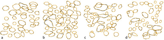
Figure 1.
The original bubble edges labeling (black) compared to best-fitting shapes reconstructed by our model (orange): (a) Low-density bubble distribution under uniform flow conditions; (b) Moderate-density bubble distribution showing slight overlaps; (c) High-density bubble distribution with significant overlaps; (d) Irregular bubble shapes under non-uniform flow conditions.
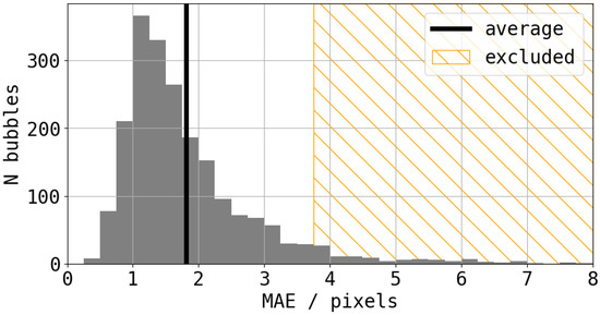
Figure 2.
Mean absolute reconstruction error distribution for the best-fitting Superformula parameters. The orange hatched region corresponds to the bubbles excluded in further analysis. The vertical solid black line represents the average MAE over the dataset.
2.3. Artificial Bubble Images Generation Framework
This subsection outlines the framework for generating artificial bubble images. We first describe the method used to generate the edges of the bubbles, followed by a discussion on how the inner pixels are filled. Lastly, we present the algorithm for generating artificial images containing multiple bubbles.
2.3.1. Shape of a Border
The fitting procedure outlined in Section 2.2 yielded a set of optimal parameters for each object in our sample. This collection of parameters allowed us to estimate the distribution in the parameter space in a data-driven manner. By mapping this distribution to a Gaussian, we subsequently constructed a generator of bubble edges.
As the fitted parameters were correlated, we first applied an orthogonal linear transformation to the parameter space in order to diagonalize the covariance matrix:
Now, is a 7-dimensional space of independent features, which can be easily mapped to the Superformula parameter space using the inverse linear transformation .
Using sklearn.preprocessing.QuantileTransformer [40], we mapped to a multivariate normal distribution :
Note that T is non-linear but still an invertible transformation, for which the parameters were fitted to distribution (and thus determined by our training dataset).
A superposition of inverse transformations , thus, mapped normal-distributed vectors to a proper data-driven distribution of Superformula parameters:
Using Q and T, we generated bubbles of a plausible shape, following this algorithm:
- Generate a sample of 7-dimensional random Gaussian vectors ;
- Map these vectors to the parameter space, using ;
- Inherit a sample of periodic functions .
2.3.2. Inner Region Intensity
Each real/artificial bubble was mapped to a unit disk using the transformation defined by Equation (10):
We generated 64 × 64 pixel images for each unit disk corresponding to a real bubble, masking the region where by setting it to zero intensity. The intensities in the generated images were normalized using the mean () and standard deviation () of intensity across all full-size images in the training dataset.
We then fit our background intensity profile model to this new dataset, performing the fit individually for each image and minimizing MSE loss over the region where :
Finally, for each model parameter in (11), that is, , , , and , we computed its mean and standard deviation across the sample (see Table 1). When generating artificial bubble images, we sampled the parameters from a Gaussian distribution based on the corresponding mean and standard deviation.

Table 1.
Best-fitting parameters of the background intensity profiles.
In real bubble images, we observed that the intensity profile often deviated from the shape of the border. To address this in our generator, we incorporated an additional shadowing effect to better replicate the observed intensity variations. We define the shadowing function:
In our generator, we sampled from a uniform distribution . The resulting shadowed intensity profile is defined as follows:
Using the generated intensity profile, we transformed back to the original polar coordinate system and intensity units . We then filled the inner region of the artificial bubbles accordingly and added Gaussian noise .
2.3.3. Artificial Images
The generation algorithm for an artificial image of size pixels consisted of the following steps:
- Fill the artificial image with Gaussian noise sampled from , and apply a Gaussian filter using a blur parameter k as a standard deviation for the Gaussian kernel. We intentionally made the background brighter by to improve the contrast in the resulting pictures. In our implementation, we fixed , , , ;
- Sample the number of bubbles from a uniform distribution . For our calculations, we set , ;
- Generate the edges of the bubbles according to the algorithm detailed in Section 2.3.1;
- Apply random rotations to the bubble edges by sampling the rotation angle from the uniform distribution ;
- Apply random shifts to the bubble centroids, with the centroid position sampled from the 2D uniform distribution ;
- Calculate the intensities of the inner regions of the bubbles using the algorithm described in Section 2.3.2. At this step, we manually multiply by a blur factor k to maintain the correct sharpness in the resulting image;
- Iteratively fill the artificial image with bubbles, using the opacity parameter :We fix in our calculations;
- Apply a Gaussian filter using our blur parameter k as a standard deviation for the Gaussian kernel;
- Clip the resulting intensity array and discretize it so that .
The corresponding labels describing the bubble edges are also generated and stored in memory after Step 4.
2.4. Combined Usage of Image Generator and CFD Modeling
It is possible to use computational fluid dynamics (CFD) results for modeling the deformable bubble shape characteristic of specific medium conditions to evaluate the ability to generate artificial bubbles. For these purposes, we performed test simulations of the form. The modeling domain consisted of a cube filled with water with sides of 1 cm and a bubble filled with gas with a diameter of 1 or 2 mm. Periodic boundary conditions were set on all cubic faces to model the motion of a single bubble rising in a continuous fluid flow. All of the values of the physical parameters, including bubble size, were taken from experiments conducted by our team at the bioreactor.
Modeling was performed using the Level-Set method [41,42,43] which allowed for modeling the motion of the boundaries of different phases using a fixed grid. Unlike other methods implemented in COMSOL Multiphysics, this method had a number of advantages, namely, accurate tracking of motion and changes in the shape of the gas bubble in the liquid, the lack of explicit tracking of boundaries, and rearrangement of the grid, which greatly simplified the modeling of complex dynamic systems, including in computational terms, and provided stable calculations even with sharp changes in the shape of the interface or the speed of its movement. This is achieved by regularizing the level function, which avoids problems with numerical instability. Moreover, COMSOL Multiphysics shows more accurate results for modeling hydrodynamic processes, especially bubble popping, which we considered in this paper, similar to this study [36]. The motion of the bubble directed by the fluid flow and the fluid flow field are described by incompressible Navier–Stokes equations and continuity equations
where is the density of the liquid phase, u is the velocity vector, t is time, p is pressure, is dynamic viscosity, I is the identity matrix, and T is transposition. F is the sum of the forces acting on the bubble, namely the drag force, the lift force, and the added mass force.
To model the motion of a single air bubble in a fluid flow, a conservative type of Level-Set equation was used to move domain boundaries of the following form:
where is a smoothing function with values 1 for one phase and 0 for the other, is a parameter of the number of repeated initializations of Level Set, is a parameter controlling the thickness of the boundary, where the value of the variable varies from 0 to 1; the finer this region, the more accurate the shape of the free surface of the object under consideration. The equations of this method were solved using the PARDISO solver, the computational grid was chosen automatic type normal (variation of cell sizes from 0.2 mm to 0.67 mm), the relationship between pressure and velocity was based on the scheme P1 + P1, and the model considered a turbulent flow model .
Numerical calculations were performed using the supercomputer ‘URAN’ of IMM UB RAS, Ekaterinburg, Russia.
3. Results
Figure 3 demonstrates four random images of the generated artificial dataset compared with four random images of real bubbles from the training dataset. One can see that the framework (see Figure 4) proposed in this study produced quite realistic images.
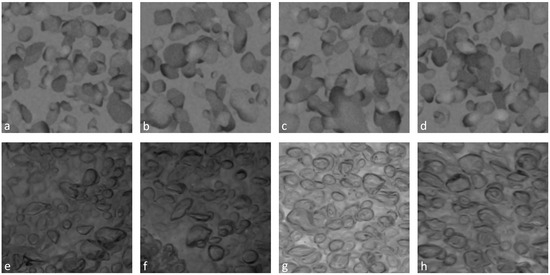
Figure 3.
Artificial bubble images generated using the framework discussed in detail in Section 2.3 (a–d) compared with the images from the training set (corresponded panels (e–h)).
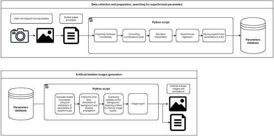
Figure 4.
Framework usage diagram.
The average time for manual annotation of a single real image for neural network training is in the order of minutes. While the automatic generation of an artificial dataset using the presented framework took a similar amount of time, it occured in automated mode and offered variability close to unlimited. Meanwhile, datasets based on manual annotation of video images are limited by the duration of video recordings and hardware capabilities. This framework significantly reduces annotation costs by requiring less manual effort, allows for the generation of large and diverse datasets for training and validation, and enables the building of a machine learning pipeline with a small number of manually labeled images or even without them. These factors lead to a reduction in data annotation costs and an increase in dataset size for training and validation, ultimately improving the performance of computer vision models.
Figure 5 shows a diagram with different bubble shapes formed under different physical properties of the medium and forces acting on the bubble. The diagram is drawn in coordinates of Reynolds number () and Eötvös (Bond) number (). Here, —liquid density; —liquid viscosity; —difference in density of the two phases; a—bubble acceleration; d—bubble diameter, —surface tension. This type of diagrams (also known as the bubble regimes plot) is widespread in the literature and is widely studied experimentally (e.g., ref. [44]).
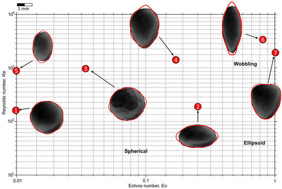
Figure 5.
Diagram with bubbles obtained by CFD modeling for different regimes of Reynolds and Eötvös numbers. Red lines show the contours of artificial bubbles generated using the presented framework.
The shape of the bubbles was modeled for the conditions presented in Table 2 using the algorithm from Section 2.4. For the modeled bubbles (dark images in Figure 5), their artificial doubles (red outline around in Figure 5) were constructed. The matching of CFD modelled and artificial bubbles is presented in Table 2.
Table 2.
Parameters of CFD simulations and related artificial bubbles.
The above results suggest that the framework allowed us to analytically describe the bubble shape with a high accuracy over a wide range of hydrodynamic conditions. This makes it possible, for example, to set plausible initial conditions for solving CFD problems using the Superformula without the necessity of preliminary equilibration of the water–bubble system. These results also show that it is possible to solve the inverse problem: by fitting the bubble shape using the Superformula, one can determine the place of such a bubble on the Reynolds–Eötvös diagram.
4. Discussion
The challenge of constructing arbitrarily shaped artificial particles is highly sought after in various scientific and technological fields. Recently, this issue has gained significant attention in the study of bubble media, where a promising avenue is the development of computer vision systems powered by neural networks for monitoring and analyzing bubble flows. The training and optimization of these systems demand extensive datasets containing labeled bubbles of diverse shapes. Obtaining such datasets experimentally is a challenging, costly, and time-intensive process. The findings of this study demonstrate that datasets can be efficiently generated using a bubble generator, which produces plausible bubble shapes that closely align with the experimentally observed data. Moreover, the number of unique samples that can be generated is virtually unlimited, enabling high-quality training and further refinement of neural networks for computer vision algorithms.
It is well known that accurately modeling bubble flows using CFD techniques is challenging due to the complex nonlinear interactions between fluid dynamics, bubble morphology, and their interaction mechanics. To facilitate advanced modeling, digital CFD twins of the bubble media are constructed. The proposed algorithm significantly simplifies this process by utilizing a family of plausible artificial bubbles as an initial approximation of the bubble medium. This approach ensures that the initial approximation is closer to the medium’s equilibrium state, eliminating the need for prolonged preliminary simulations. The results of this study demonstrate that artificial bubbles can replicate those generated by CFD simulations with an accuracy of at least 95%.
CFD simulations, on the other hand, provide detailed insights into hydrodynamic conditions. For instance, in the diagram (Figure 5), bubbles of various shapes within the dimensionless space of Reynolds and Eötvös numbers are shown. This offers the potential for future generation of realistic bubbles as a function of hydrodynamic parameters, similar to the approach taken in [45].
A key advantage of CFD simulations is their ability to produce three-dimensional, undistorted bubble shapes. In contrast, video data are constrained by the limitations of optical equipment, where bubbles may overlap, and lighting effects can distort their appearance. As a result, video data are often processed as a two-dimensional projection of bubbles. The Superformula, however, can be extended to a three-dimensional form as outlined in [46], enabling the generation of fully three-dimensional, asymmetric bubbles that enhance video-based observations with 3D details.
The ability to generate artificial bubble images using Superformula regression offers a novel approach to improving mass transfer efficiency in chemical and biological bubble reactors. In these systems, the structure of the bubble medium is crucial for ensuring effective gas exchange, as the chemical or biological reactions rely on the accurate delivery of dissolved oxygen to the target medium. By employing more precise bubble detection through advanced neural network training, it becomes possible to accurately assess key processes such as oxygen transfer, mixing dynamics, and the control of gas–liquid interfaces—factors that directly influence reactor performance.
Beyond bubble environments, the potential for analytically describing the shape of 3D objects (via fitting with an analytical surface description) within this framework is highly promising for images obtained from tomography techniques. When scanning small objects such as bubbles, droplets, casting defects, or biological tissues, a common challenge is low image resolution combined with artifacts and noise. In such cases, the framework’s capabilities can be leveraged for optimal interpolation, image smoothing, and the reconstruction of 3D objects.
5. Conclusions
This study presents an innovative approach to solving the challenges associated with generating datasets of bubble media images, essential for training neural network algorithms for bubble detection in multiphase systems. Given that no universal or fully robust neural network currently exists for such tasks, existing models rely on large, manually labeled datasets for retraining, a labor-intensive and time-consuming process. To address this limitation, we propose a novel artificial bubble imaging method, capable of generating significant datasets to enhance and refine neural network models.
By employing Superformula regression, we generate realistic artificial bubble images that closely replicate the shapes and dynamics of gas–liquid inclusions. While the Superformula forms the foundation of this method, it can be substituted with other approximation formulas to accommodate more complex bubble geometries. This method holds significant potential for biotechnology, particularly in optimizing bioreactor performance and enhancing bioprotein production. The ability to generate artificial bubble images provides a novel pathway for improving mass transfer efficiency, a critical factor for ensuring adequate gas exchange in systems where microbial growth depends on precise oxygen delivery. By enabling more accurate bubble detection through advanced neural network training, this framework supports the fine-tuning of essential processes like oxygen transfer, mixing dynamics, and gas–liquid interface control—key factors that directly impact bioreactor productivity.
Moreover, the generated images serve two primary purposes: first, as training data to improve neural network accuracy in detecting bubbles under real-world conditions, and second, as input data for hydrodynamic modeling, including post-processing in CFD simulations. In real-world bioprotein production, where efficient gas exchange is vital for scaling operations and maximizing yields, this methodology provides tools to better understand and simulate bubble behavior. This facilitates more effective control of bioprocesses and allows for real-time adjustments to gas–liquid flows.
The performance of the proposed framework was quantitatively evaluated to validate its effectiveness. For the border detection method using Superformula regression, the mean absolute error (MAE) between the reconstructed and ground truth bubble shapes was 1.82 pixels, representing a 25% improvement in accuracy compared with the baseline classical algorithms. Furthermore, the artificial bubble image generation framework demonstrated a shape matching accuracy of at least 95% when compared with computational fluid dynamics (CFD) simulations of bubble shapes under various hydrodynamic conditions. This high level of accuracy ensures that the generated datasets are suitable for training neural networks with minimal need for manual annotation. Additionally, the time required for manual annotation of video data was reduced by over 50%, significantly accelerating the preparation of training datasets for computer vision applications.
With further refinement, this framework could become an integral part of the design and operation of large-scale bioreactors, contributing to more sustainable and efficient production of bioproteins and other bio-based products. By enhancing the analysis and modeling of multiphase systems, our approach addresses the limitations of current bubble detection methods and offers a promising tool for future developments in computer vision, neural network training, and multiphase system modeling.
Author Contributions
Conceptualization, I.N.; methodology, P.M.; software, P.M. and N.M.; formal analysis, P.M.; investigation, M.N.; resources, D.C. and I.S.; writing—original draft preparation, I.S. and I.N.; writing—review and editing, I.S. and S.L.; visualization, K.M.; project administration, I.N.; funding acquisition, I.S. All authors have read and agreed to the published version of the manuscript.
Funding
This study was supported by the Russian Science Foundation (project no. 24-11-00351).
Data Availability Statement
The original contributions presented in this study are included in the article. Further inquiries can be directed to the corresponding authors.
Conflicts of Interest
Author Dmitrii Chernushkin was employed by the company NPO Biosintez Ltd. The remaining authors declare that the research was conducted in the absence of any commercial or financial relationships that could be construed as a potential conflict of interest.
References
- Qiao, C.; Yang, D.; Mao, X.; Xie, L.; Gong, L.; Peng, X.; Peng, Q.; Wang, T.; Zhang, H.; Zeng, H. Recent advances in bubble-based technologies: Underlying interaction mechanisms and applications. Appl. Phys. Rev. 2021, 8, 011315. [Google Scholar] [CrossRef]
- Walls, P.; McRae, O.; Natarajan, V.; Johnson, C.; Antoniou, C.; Bird, J. Quantifying the potential for bursting bubbles to damage suspended cells. Sci. Rep. 2017, 7, 15102. [Google Scholar] [CrossRef] [PubMed]
- Patel, A.K.; Singhania, R.R.; Chen, C.W.; Tseng, Y.S.; Kuo, C.H.; Wu, C.H.; Dong, C.D. Advances in micro- and nano bubbles technology for application in biochemical processes. Environ. Technol. Innov. 2021, 23, 101729. [Google Scholar] [CrossRef]
- Hun, L.J. Bubble Arresting and Recycling Method and Facilities for Biological Reactors of Wastewater Treatment Plants. Korea Institute of Construction Technology Patent KR20040051785A, 19 June 2004. Available online: https://patents.google.com/patent/KR20040051785A/en (accessed on 23 December 2024).
- Andrews, G.; Apel, W. Bioreactors, Gas Treatment. In Encyclopedia of Bioprocess Technology; John Wiley & Sons: Hoboken, NJ, USA, 2010. [Google Scholar] [CrossRef]
- Gilmour, D.J.; Zimmerman, W.B. Microbubble intensification of bioprocessing. Adv. Microb. Physiol. 2020, 77, 1–35. [Google Scholar] [CrossRef]
- Kováts, P.; Thévenin, D.; Zähringer, K. Characterizing fluid dynamics in a bubble column aimed for the determination of reactive mass transfer. Heat Mass Transf. 2018, 54, 453–461. [Google Scholar] [CrossRef]
- Peterat, G.; Schmolke, H.; Lorenz, T.; Llobera, A.; Rasch, D.; Al-Halhouli, A.; Dietzel, A.; Büttgenbach, S.; Klages, C.P.; Krull, R. Characterization of oxygen transfer in vertical microbubble columns for aerobic biotechnological processes. Biotechnol. Bioeng. 2014, 111, 1809–1819. [Google Scholar] [CrossRef]
- Goldobin, D.S.; Brilliantov, N.V. Diffusive counter dispersion of mass in bubbly media. Phys. Rev. E 2011, 84, 056328. [Google Scholar] [CrossRef]
- Martínez, A.M.M.; Silva, E.M.E. Airlift Bioreactors: Hydrodynamics and Rheology Application to Secondary Metabolites Production. In Mass Transfer: Advances in Sustainable Energy and Environment Oriented Numerical Modeling; Intech: Rijeka, Croatia, 2013. [Google Scholar] [CrossRef]
- Mei, L.; Chen, X.; Zhang, Z.; Liang, J.Z.; Wei, X.; Wang, L. Experimental Study on Bubble Dynamics and Mass Transfer Characteristics of Coaxial Bubbles in Petroleum-Based Liquids. ACS Omega 2023, 8, 17159–17170. [Google Scholar] [CrossRef]
- Sojahrood, A.J.; Earl, R.; Li, Q.; Porter, T.M.; Kolios, M.C.; Karshafian, R. Nonlinear dynamics of acoustic bubbles excited by their pressure dependent subharmonic resonance frequency: Oversaturation and enhancement of the subharmonic signal. arXiv 2019, arXiv:1909.05071. [Google Scholar]
- Vesipa, R.; Paissoni, E.; Manes, C.; Ridolfi, L. Dynamics of bubbles under stochastic pressure forcing. Phys. Rev. E 2021, 103, 023108. [Google Scholar] [CrossRef]
- Beltrán-Prieto, J.C.; Beltrán-Prieto, L.A. Mathematical Model for Mass Transfer Coefficient Determination in Dissolution Process. WSEAS Trans. Heat Mass Transf. 2017, 12, 86–92. [Google Scholar]
- Ren, Z.; Li, D.; Wang, H.; Liu, J.; Li, Y. Computational model for predicting the dynamic dissolution and evolution behaviors of gases in liquids. Phys. Fluids 2022, 34, 103310. [Google Scholar] [CrossRef]
- Kracík, T.; Moucha, T.; Petříček, R.; Petříček, R. Gas-Liquid Contactors’ Aeration Capacities When Agitated by Rushton Turbines of Various Diameters. ACS Omega 2020, 5, 5072–5077. [Google Scholar] [CrossRef]
- Sano, Y.; Yamaguchi, N.; Adachi, T. Mass transfer coefficients for suspended particles in agitated vessels and bubble columns. J. Chem. Eng. Jpn. 1974, 7, 255–261. [Google Scholar] [CrossRef]
- Kataoka, H.; Takeuchi, H.; Nakao, K.; Yagi, H.; Tadaki, T.; Otake, T.; Miyauchi, T.; Washimi, K.; Watanabe, K.; Yoshida, F. Mass transfer in a large bubble column. J. Chem. Eng. Jpn. 1979, 12, 105–110. [Google Scholar] [CrossRef][Green Version]
- Popović, M.; Robinson, C.W. Mass transfer studies of external-loop airlifts and a bubble column. Aiche J. 1989, 35, 393–405. [Google Scholar] [CrossRef]
- Bouaifi, M.; Roustan, M. Bubble size and mass transfer coefficients in dual-impeller agitated reactors. Can. J. Chem. Eng. 1998, 76, 390–397. [Google Scholar] [CrossRef]
- Cockx, A.; Roustan, M.; Liné, A.; Hébrard, G. Modelling of mass transfer coefficient KL in bubble columns. Chem. Eng. Res. Des. 1995, 73, 627–631. [Google Scholar] [CrossRef]
- Huang, G.; Lv, X.; Chen, W.C.; Song, Y.; Yin, J.; Wang, D. Measurement of interfacial mass transfer of single bubbles rising in homogeneous turbulence. Chem. Eng. Sci. 2024, 288, 119757. [Google Scholar] [CrossRef]
- Farsoiya, P.K.; Magdelaine, Q.; Antkowiak, A.; Popinet, S.; Deike, L. Direct numerical simulations of bubble-mediated gas transfer and dissolution in quiescent and turbulent flows. J. Fluid Mech. 2023, 954, A29. [Google Scholar] [CrossRef]
- Nizovtseva, I.; Palmin, V.; Simkin, I.; Starodumov, I.; Mikushin, P.; Nozik, A.; Hamitov, T.; Ivanov, S.; Vikharev, S.; Zinovev, A.; et al. Assessing the Mass Transfer Coefficient in Jet Bioreactors with Classical Computer Vision Methods and Neural Networks Algorithms. Algorithms 2023, 16, 125. [Google Scholar] [CrossRef]
- Gan, J.; Liu, H.; Wei, Y.; Chen, J.; Li, X.; Jiang, Z.; Li, G.; Li, H.; Chen, K. Bubble Diameter, Mass Transfer, and Bioreaction of Dynamic Membrane-Stirred Reactors. Ind. Eng. Chem. Res. 2024, 63, 1760–1772. [Google Scholar] [CrossRef]
- Volger, R.; Puiman, L.; Haringa, C. Bubbles and Broth: A review on the impact of broth composition on bubble column bioreactor hydrodynamics. Biochem. Eng. J. 2023, 201, 109124. [Google Scholar] [CrossRef]
- Starodumov, I.; Sokolov, S.; Mikushin, P.; Nikishina, M.; Mityashin, T.; Makhaeva, K.; Blyakhman, F.; Chernushkin, D.; Nizovtseva, I. Computer Vision Algorithm for Characterization of a Turbulent Gas–Liquid Jet. Inventions 2024, 9, 9. [Google Scholar] [CrossRef]
- Nizovtseva, I.G.; Starodumov, I.O.; Lezhnin, S.I.; Mikushin, P.V.; Zagoruiko, A.N.; Shabadrov, P.A.; Svitich, V.Y.; Vikharev, S.V.; Tatarintsev, V.V.; Nikishina, M.A.; et al. Influence of the gas–liquid non-equilibrium media structure on the mass transfer dynamics in biophysical processes. Smart Mater. Struct. 2023, 33, 015028. [Google Scholar] [CrossRef]
- Starodumov, I.; Nizovtseva, I.; Lezhnin, S.; Vikharev, S.; Svitich, V.; Mikushin, P.; Alexandrov, D.; Kuznetsov, N.; Chernushkin, D. Measurement of Mass Transfer Intensity in Gas–Liquid Medium of Bioreactor Circuit Using the Thermometry Method. Fluids 2022, 7, 366. [Google Scholar] [CrossRef]
- Starodumov, I.; Ankudinov, V.; Nizovtseva, I. A review of continuous modeling of periodic pattern formation with modified phase-field crystal models. Eur. Phys. J. Spec. Top. 2022, 231, 1135–1145. [Google Scholar] [CrossRef]
- Hamilton, R.; Irina, N.; Dmitri, C.; Kalyuzhnaya, M.G. C1-Proteins Prospect for Production of Industrial Proteins and Protein-Based Materials from Methane; CRC Press: Boca Raton, FL, USA, 2022. [Google Scholar]
- Liebendorfer, A.P. Deep learning algorithms identify and track bubbles through gas-liquid interfaces in real time. Scilight 2024, 2024, 321107. [Google Scholar] [CrossRef]
- Fang, L.; Ning, J.; Zhang, J.; Feng, Y. A deep learning-based algorithm for rapid tracking and monitoring of gas–liquid two-phase bubbly flow bubbles. Phys. Fluids 2024, 36, 083316. [Google Scholar] [CrossRef]
- Bellini, F.; Gonon, L.; Mazzon, A.; Meyer-Brandis, T. Detecting asset price bubbles using deep learning. Math. Financ. 2024. [Google Scholar] [CrossRef]
- Gupta, R.; Fletcher, D.F.; Haynes, B.S. CFD modelling of flow and heat transfer in the Taylor flow regime. Chem. Eng. Sci. 2010, 65, 2094–2107. [Google Scholar] [CrossRef]
- Crha, J.; Basarova, P.; Ruzicka, M.; Kaspar, O.; Zedníková, M. Comparison of Two Solvers for Simulation of Single Bubble Rising Dynamics: COMSOL vs. Fluent. Minerals 2021, 11, 452. [Google Scholar] [CrossRef]
- Gielis, J. A generic geometric transformation that unifies a wide range of natural and abstract shapes. Am. J. Bot. 2003, 90, 333–338. [Google Scholar] [CrossRef] [PubMed]
- Dwyer, B.; Nelson, J.; Hansen, T. Roboflow, Version 1.0. 2024. Available online: https://roboflow.com (accessed on 23 December 2024).
- Kingma, D.P.; Ba, J. Adam: A Method for Stochastic Optimization. arXiv 2014, arXiv:1412.6980. [Google Scholar]
- Pedregosa, F.; Varoquaux, G.; Gramfort, A.; Michel, V.; Thirion, B.; Grisel, O.; Blondel, M.; Prettenhofer, P.; Weiss, R.; Dubourg, V.; et al. Scikit-learn: Machine learning in Python. J. Mach. Learn. Res. 2011, 12, 2825–2830. [Google Scholar]
- Sussman, M.; Smereka, P.; Osher, S. A level set approach for computing solutions to incompressible two-phase flow. J. Comput. Phys. 1994, 114, 146–159. [Google Scholar] [CrossRef]
- Yu, Z.; Fan, L.S. Direct simulation of the buoyant rise of bubbles in infinite liquid using level set method. Can. J. Chem. Eng. 2008, 86, 267–275. [Google Scholar] [CrossRef]
- Suh, Y.; Son, G. A level-set method for simulation of a thermal inkjet process. Numer. Heat Transf. Part Fundam. 2008, 54, 138–156. [Google Scholar] [CrossRef]
- Bhaga, D.; Weber, M. Bubbles in viscous liquids: Shapes, wakes and velocities. J. Fluid Mech. 1981, 105, 61–85. [Google Scholar] [CrossRef]
- Haas, T.; Schubert, C.; Eickhoff, M.; Pfeifer, H. A Review of Bubble Dynamics in Liquid Metals. Metals 2021, 11, 664. [Google Scholar] [CrossRef]
- Zhou, S.; Li, Q.; Townsend, S.; Xie, Y.; Huang, X. Design of Novel Nanoparticles for Thin-Film Solar Cells. In Proceedings of the 10th World Congress on Structural and Multidisciplinary Optimization, Orlando, FL, USA, 19–24 May 2013. [Google Scholar]


Disclaimer/Publisher’s Note: The statements, opinions and data contained in all publications are solely those of the individual author(s) and contributor(s) and not of MDPI and/or the editor(s). MDPI and/or the editor(s) disclaim responsibility for any injury to people or property resulting from any ideas, methods, instructions or products referred to in the content. |
© 2024 by the authors. Licensee MDPI, Basel, Switzerland. This article is an open access article distributed under the terms and conditions of the Creative Commons Attribution (CC BY) license (https://creativecommons.org/licenses/by/4.0/).