On a Family of Hamilton–Poisson Jerk Systems

Abstract

In this paper, we construct a family of Hamilton–Poisson jerk systems. We show that such a system has infinitely many Hamilton–Poisson realizations. In addition, we discuss the stability and we prove the existence of periodic orbits around nonlinearly stable equilibrium points. Particularly, we deduce conditions for the existence of homoclinic and heteroclinic orbits. We apply the obtained results to a family of anharmonic oscillators.

1. Introduction

Jerk is the rate of change of acceleration, the third derivative of position with respect to time [1]. A jerk equation $\stackrel{⃛}{x}=j(x,\dot{x},\ddot{x})$ and the corresponding jerk system, which is a three-dimensional system given by

$$\left\{\begin{array}{c}\dot{x}=y\hfill \\ \dot{y}=z\hfill \\ \dot{z}=j(x,y,z)\hfill \end{array}\right.,$$

(1)

can model processes characterized by changes in acceleration. Despite their simple form, jerk systems provide examples of chaotic behavior (see, e.g., [2,3,4]). Bifurcations in the dynamics of jerk systems are also analyzed (see, e.g., [5,6,7,8]).

In this paper, we study how Hamilton–Poisson jerk systems can be constructed. Roughly speaking, a three-dimensional system is a Hamilton–Poisson system if it has two independent constants of motion (for details on Hamilton–Poisson mechanics, see e.g., [9]). Using such functions, we obtain a family of Hamilton–Poisson jerk systems, given by $\stackrel{⃛}{x}+f^{\prime }\left(x\right)\dot{x}=0$, which are in fact jerk versions of the system with one degree of freedom $\ddot{x}+f\left(x\right)=0$ [10]. For instance, the equations of the harmonic oscillator, the mathematical pendulum, the Duffing oscillator, and other anharmonic oscillators are of this form.

Oscillatory systems, characterized by repetitive patterns or cycles, are found in various biological phenomena such as circadian rhythms (see, e.g., [11]), neuronal activity (see, e.g., [12]), and even in cellular processes like metabolic oscillations (see, e.g., [13]). Population dynamics in predator–prey relationships often display cyclic behavior, where changes in predator and prey populations exhibit periodic patterns (see, e.g., [14]). Modeling changes in population sizes or ecological systems often involves sudden shifts or rapid changes in growth rates, which can be compared analogously to jerk-like behavior in dynamic systems. Moreover, in neural systems, sudden changes in firing rates or neuronal activities might indirectly relate to rapid changes in behavior akin to jerk-like dynamics.

The paper is organized as follows: in Section 2, we recall some notions regarding Hamilton–Poisson systems and then we give some conditions for which system (1) is of this type. Using the integrable deformation method (see [15] and references therein), we construct a family of Hamilton–Poisson jerk systems. Also, we give Hamilton–Poisson realizations of such a system. In Section 3, we analyze some dynamical properties of the obtained system, namely, the stability of the equilibrium points, the existence of the periodic orbits around some nonlinearly stable equilibria, and the existence of homoclinic or heteroclinic orbits. In Section 4, we apply these results to a family of anharmonic oscillators [16].

2. A Family of Hamilton–Poisson Jerk Systems

In this section, we construct a family of jerk systems that have Hamilton–Poisson realizations.

Recall that the three-dimensional dynamical system

$$(\dot{x},\dot{y},\dot{z})=(f_1(x,y,x),f_2(x,y,z),f_3(x,y,z))$$

is a Hamilton–Poisson system on ${\mathbb{R}}^3$ if there are the smooth functions $\nu ,H,C$ such that

$${(f_1,f_2,f_3)}^T=\nu \nabla H\times \nabla C$$

on ${\mathbb{R}}^3$ (see, e.g., [17,18]). The function $\nu$ is called the rescaling function. In addition, the Hamiltonian function H and the Casimir function C are constants of motion of the above system. In fact, a Hamilton–Poisson system on ${\mathbb{R}}^3$ is a triple $({\mathbb{R}}^3,\mathrm{\Pi },H)$, where $\mathrm{\Pi }$ is a Poisson structure, and in this case it is given by the matrix

$$\mathrm{\Pi }=\nu \left[\begin{array}{ccc}0& C_z& -C_y\\ -C_z& 0& C_x\\ C_y& -C_x& 0\end{array}\right],$$

(2)

where we have denoted $C_x=\frac{\partial C}{\partial x}$. Such a system writes ${(\dot{x},\dot{y},\dot{z})}^t=\mathrm{\Pi }·\nabla H.$ Details on Hamiltonian mechanics can be found, for example, in [19].

In the following, we consider $\nu =1$. One of our goals is to obtain jerk systems that can be written in the form ${(\dot{x},\dot{y},\dot{z})}^T=\nabla H\times \nabla C,$ that is, to determine functions $H,C$ such that

$$\begin{array}{cc}\hfill & H_y{C}_z-H_z{C}_y=y\hfill \\ \hfill & H_z{C}_x-H_x{C}_z=z\hfill \\ \hfill & H_x{C}_y-H_y{C}_x=j(x,y,z),\hfill \end{array}$$

and which are constants of motion of system (1), that is,

$$\begin{array}{cc}\hfill & y{H}_x+z{H}_y+j(x,y,z)H_z=0\hfill \\ \hfill & y{C}_x+z{C}_y+j(x,y,z)C_z=0.\hfill \end{array}$$

We note that achieving this goal appears to be complicated for a general jerk function $j.$ However, the next result holds.

Theorem 1.

If $j_z\ne 0,$ then jerk system (1) cannot have a Hamilton–Poisson formulation ${(\dot{x},\dot{y},\dot{z})}^T=\nabla H\times \nabla C.$

Proof. 

On the one hand, the divergence of system (1) is $div(y,z,j(x,y,z))=j_z$. On the other hand, $div(\nabla H\times \nabla C)=\nabla ·(\nabla H\times \nabla C)=0$; thus, $j_z=0$, which finishes the proof. □

Instead of starting with a function j and checking for the existence of the functions H and C, we can construct Hamilton–Poisson jerk systems using integrable deformation method [15].

Consider the jerk equation

$$\stackrel{⃛}{x}=0$$

and the corresponding jerk system

$$\left\{\begin{array}{c}\dot{x}=y\hfill \\ \dot{y}=z\hfill \\ \dot{z}=0\hfill \end{array}\right..$$

(3)

It is easy to see that the functions

$$H(x,y,z)={\displaystyle \frac{1}{2}}{y}^2-xz,C(x,y,z)=z$$

are constants of motion for system (3). Moreover, system (3) writes ${(\dot{x},\dot{y},\dot{z})}^T=\nabla H\times \nabla C$; thus, it has the Hamilton–Poisson realization $({\mathbb{R}}^3,\mathrm{\Pi },H)$ with the Hamiltonian H and the Poisson structure given by the matrix

$$\mathrm{\Pi }=\left[\begin{array}{ccc}0& 1& 0\\ -1& 0& 0\\ 0& 0& 0\end{array}\right].$$

Now, we alter the above Hamiltonian and Casimir functions, that is, we consider the functions

$$\begin{array}{cc}\hfill & \tilde{H}(x,y,z)=H(x,y,z)+g_1\alpha (x,y,z)={\displaystyle \frac{1}{2}}{y}^2-xz+g_1\alpha (x,y,z),\hfill \end{array}$$

(4)

$$\begin{array}{cc}\hfill & \tilde{C}(x,y,z)=C(x,y,z)+g_2\beta (x,y,z)=z+g_2\beta (x,y,z),\hfill \end{array}$$

(5)

where $\alpha$ and $\beta$ are smooth, and $g_1,g_2$ are real parameters. Then, an integrable deformation of system (3) is given by

$${(\dot{x},\dot{y},\dot{z})}^T=\nabla \tilde{H}\times \nabla \tilde{C},$$

(6)

that is

$$\left\{\begin{array}{c}\dot{x}=y+g_2(y{\beta }_z+x{\beta }_y)+g_1{\alpha }_y+g_1{g}_2({\alpha }_y{\beta }_z-{\alpha }_z{\beta }_y)\hfill \\ \dot{y}=z+g_2(z{\beta }_z-x{\beta }_x)-g_1{\alpha }_x+g_1{g}_2(-{\alpha }_x{\beta }_z+{\alpha }_z{\beta }_x)\hfill \\ \dot{z}=g_2(-z{\beta }_y-y{\beta }_x)+g_1{g}_2({\alpha }_x{\beta }_y-{\alpha }_y{\beta }_x)\hfill \end{array}\right..$$

(7)

System (7) is jerk only if

$$\left\{\begin{array}{c}{g}_2(y{\beta }_z+x{\beta }_y)+g_1{\alpha }_y+g_1{g}_2({\alpha }_y{\beta }_z-{\alpha }_z{\beta }_y)=0\hfill \\ g_2(z{\beta }_z-x{\beta }_x)-g_1{\alpha }_x+g_1{g}_2(-{\alpha }_x{\beta }_z+{\alpha }_z{\beta }_x)=0\hfill \end{array}\right..$$

(8)

Now, we choose

$$\alpha (x,y,z)=\alpha (x,y),\beta (x,y,z)=\beta (x,y),$$

and (8) turns into

$$\left\{\begin{array}{c}{g}_1{\alpha }_y=-g_{2}x{\beta }_y\hfill \\ g_1{\alpha }_x=-g_{2}x{\beta }_x\hfill \end{array}\right..$$

Then,

$$\left\{\begin{array}{c}{g}_1{\alpha }_{xy}=-g_2({\beta }_y+x{\beta }_{xy})\hfill \\ g_1{\alpha }_{xy}=-g_{2}x{\beta }_{xy}\hfill \end{array}\right.,$$

thus, ${\beta }_y=0$ and, consequently, ${\alpha }_y=0.$ Therefore,

$$\alpha (x,y,z)=\alpha \left(x\right),\beta (x,y,z)=\beta \left(x\right).$$

Consequently, if the functions $\alpha =\alpha \left(x\right)$ and $\beta =\beta \left(x\right)$ satisfy the relation

$$g_1{\alpha }^{\prime }\left(x\right)=-g_{2}x{\beta }^{\prime }\left(x\right),$$

(9)

then we constructed the following family of Hamilton–Poisson jerk systems

$$\left\{\begin{array}{c}\dot{x}=y\hfill \\ \dot{y}=z\hfill \\ \dot{z}=-g_{2}y{\beta }^{\prime }\left(x\right)\hfill \end{array}\right..$$

(10)

The corresponding jerk equation is given by

$$\stackrel{⃛}{x}+g_2{\beta }^{\prime }\left(x\right)\dot{x}=0.$$

(11)

The jerk versions of the most known oscillators (the harmonic oscillator $\ddot{x}+x=0$, the mathematical pendulum $\ddot{x}+sinx=0$, and the Duffing oscillator $\ddot{x}+x^3-x=0$) belong to the above family of jerk equations.

In the following, we give Hamilton–Poisson realizations of system (10). For this purpose, using (2), the functions

$$\begin{array}{cc}\hfill & C(x,y,z)=z+g_2\beta \left(x\right)\mathrm{and}H(x,y,z)={\displaystyle \frac{1}{2}}{y}^2-xz+g_1\alpha \left(x\right)\hfill \end{array}$$

(12)

give the matrices

$${\mathrm{\Pi }}_{1,0}=\left[\begin{array}{ccc}0& 1& 0\\ \\ -1& 0& g_2{\beta }^{\prime }\left(x\right)\\ \\ 0& -g_2{\beta }^{\prime }\left(x\right)& 0\end{array}\right]$$

(13)

and

$${\mathrm{\Pi }}_{0,1}=\left[\begin{array}{ccc}0& -x& -y\\ \\ x& 0& -z+g_1{\alpha }^{\prime }\left(x\right)\\ \\ y& z-g_1{\alpha }^{\prime }\left(x\right)& 0\end{array}\right],$$

(14)

respectively.

Theorem 2.

Let $\alpha ,\beta$ be smooth functions such that $g_1{\alpha }^{\prime }\left(x\right)=-g_{2}x{\beta }^{\prime }\left(x\right)$, where $g_1,g_2\in \mathbb{R}.$ Then, system (10) has the Hamilton–Poisson realizations

$$\left({\mathbb{R}}^3,{\mathrm{\Pi }}_{1,0},H\right) and\left({\mathbb{R}}^3,{\mathrm{\Pi }}_{0,1},-C\right).$$

Moreover, (10) is a bi-Hamiltonian system.

Proof. 

Using (12)–(14), it is easy to see that system (10) writes ${(\dot{x},\dot{y},\dot{z})}^T=\nabla H\times \nabla C=\nabla (-C)\times \nabla H.$ In addition, ${\mathrm{\Pi }}_{0,1}·\nabla H={\mathrm{\Pi }}_{1,0}·\nabla (-C)=\mathbf{0}$ and ${\mathrm{\Pi }}_{1,0}·\nabla H={\mathrm{\Pi }}_{0,1}\nabla (-C)={(\dot{x},\dot{y},\dot{z})}^T.$

The sum of the matrices ${\mathrm{\Pi }}_1$ and ${\mathrm{\Pi }}_2$ is a Poisson structure. Therefore, ${\mathrm{\Pi }}_1$ and ${\mathrm{\Pi }}_2$ are compatible Poisson structures, and (10) is a bi-Hamiltonian system. □

As a consequence, we obtain the next result.

Theorem 3.

Let $a,b,c,d\in \mathbb{R}$ such that $ad-bc=1$. Then, system (10) admits infinitely many Hamilton–Poisson realizations $\left({\mathbb{R}}^3,{\mathrm{\Pi }}_{a,b},H_{c,d}\right),$ where the Hamiltonian $H_{c,d}$ is given by

$$H_{c,d}=cC+dH=c\left(z+g_2\beta \left(x\right)\right)+d\left({\displaystyle \frac{y^2}{2}}-xz+g_1\alpha \left(x\right)\right),$$

the Poisson structure is defined by

$${\mathrm{\Pi }}_{a,b}=a{\mathrm{\Pi }}_{1,0}+b{\mathrm{\Pi }}_{0,1}=\left[\begin{array}{ccc}0& a-bx& -by\\ \\ -a+bx& 0& a{g}_2{\beta }^{\prime }\left(x\right)+b{g}_1{\alpha }^{\prime }\left(x\right)-bz\\ \\ by& -a{g}_2{\beta }^{\prime }\left(x\right)-b{g}_1{\alpha }^{\prime }\left(x\right)+bz& 0\end{array}\right],$$

and a Casimir of the Poisson structure is

$$C_{a,b}=aC+bH=a\left(z+g_2\beta \left(x\right)\right)+b\left({\displaystyle \frac{y^2}{2}}-xz+g_1\alpha \left(x\right)\right).$$

Since $\nabla C(x,y,z)=(g_2{\beta }^{\prime }\left(x\right),0,1)\ne (0,0,0),$ for all $(x,y,z)\in {\mathbb{R}}^3$, every level set of the Casimir function C is a regular surface. We denote such a level set by

$${\mathcal{O}}_c=C^{-1}\left(c\right)=\{(x,y,z)\in {\mathbb{R}}^3|z+g_2\beta \left(x\right)=c\}.$$

The regular symplectic leaves associated with the Poisson structure ${\mathrm{\Pi }}_{1,0}$ are given by the connected components corresponding to pre-images of regular values of the Casimir function C. Therefore, ${\mathcal{O}}_c$ is the regular symplectic leaf of the Poisson structure ${\mathrm{\Pi }}_{1,0}$ corresponding to the regular value $c\in \mathbb{R}$ of C. In addition, the dynamics of the Hamilton–Poisson system $\left({\mathbb{R}}^3,{\mathrm{\Pi }}_{1,0},H\right)$ are foliated by these symplectic leaves. Moreover, the restriction of system (10) to a regular leaf ${\mathcal{O}}_c$ is the following completely integrable Hamiltonian system $({\mathcal{O}}_c,\omega =dp\wedge dq,H{|}_{{\mathcal{O}}_c}),$ where the Hamiltonian ${H|}_{{\mathcal{O}}_c}=H(p,q)$ is given by

$$H(p,q)=\frac{1}{2}{p}^2+g_1\alpha \left(q\right)+g_{2}q\beta \left(q\right)-cq,$$

(15)

The reduced equations are

$$\left\{\begin{array}{c}\dot{q}=H_p=p\hfill \\ \dot{p}=-H_q=c-g_2\beta \left(q\right)\hfill \end{array}\right.,$$

(16)

or equivalent

$$\ddot{q}=W^{\prime }\left(q\right),$$

(17)

where $W^{\prime }\left(q\right)=c-g_2\beta \left(q\right).$

Thus, on each level set ${\mathcal{O}}_c$ the dynamics of system (10) are given by system (16) or Equation (17), representing a nonlinear oscillator with the kinetic energy $T=\frac{1}{2}{p}^2$ and the potential energy $V\left(q\right)=-W\left(q\right)=g_1\alpha \left(q\right)+g_{2}q\beta \left(q\right)-cq$ (for details about the system $\ddot{x}=f\left(x\right)$, see, e.g., [10,20]).

3. Some Dynamical Properties

In this section, we study the stability of system (10) and we prove the existence of some periodic orbits. Also, we obtain sufficient conditions for the existence of heteroclinic and homoclinic orbits.

The equilibrium points of system (10) are given by the family $\mathcal{E}=\left\{\left(M,0,0\right)|M\in \mathbb{R}\right\}.$ Now, we discuss their stability.

Theorem 4.

Let $\alpha ,\beta$ be smooth functions such that $g_1{\alpha }^{\prime }\left(x\right)=-g_{2}x{\beta }^{\prime }\left(x\right)$, where $g_1,g_2\in \mathbb{R}.$ Denote $e_M=(M,0,0)\in \mathcal{E},$ $M\in \mathbb{R}$ as an arbitrary equilibrium point of system (10). Also consider the function

$$F\left(x\right)=g_1(\alpha \left(M\right)-\alpha \left(x\right))+g_{2}x(\beta \left(M\right)-\beta \left(x\right)).$$

(18)

(i)

If $g_2{\beta }^{\prime }\left(M\right)<0$ or $g_2=0$, then the equilibrium point $e_M$ is unstable.

(ii)

If $g_2{\beta }^{\prime }\left(M\right)>0$, then the equilibrium point $e_M$ is nonlineary stable.

(iii)

If ${\beta }^{\prime }\left(M\right)=0$ and there is a neighborhood $V\subset \mathbb{R}$ of M such that $F\left(x\right)<0,$ for all $x\in V\setminus \left\{M\right\}$, then the equilibrium point $e_M$ is nonlineary stable.

(iv)

If ${\beta }^{\prime }\left(M\right)=0$ and there is a neighborhood $V=(a,b)\subset \mathbb{R}$ of M such that $F\left(x\right)>0,$ for all $x\in (a,M)$ or $x\in (M,b)$, then the equilibrium point $e_M$ is unstable.

Proof. 

The Jacobian matrix of system (10) at $e_M$ is

$$J(M,0,0)=\left[\begin{array}{ccc}0& 1& 0\\ \\ 0& 0& 1\\ \\ 0& -g_2{\beta }^{\prime }\left(M\right)& 0\end{array}\right],$$

(19)

with the characteristic polynomial

$$P_M\left(\lambda \right)=-\lambda ({\lambda }^2+g_2{\beta }^{\prime }\left(M\right))$$

(20)

and eigenvalues

$${\lambda }_1=0,{\lambda }_{2,3}=\pm \sqrt{-g_2{\beta }^{\prime }\left(M\right)}.$$

(21)

• (i) Let $g_2{\beta }^{\prime }\left(M\right)<0$. From (21), it results that one of the eigenvalues is a positive number. Therfore, $e_M$ is an unstable equilibrium point.

If $g_2=0$, system (10) becomes (3), and it has the solution

$$x\left(t\right)={\displaystyle \frac{C_1}{2}}{t}^2+C_{2}t+C_3,y\left(t\right)=C_{1}t+C_2,z\left(t\right)=C_1$$

where $C_1,C_2,C_3\in \mathbb{R}$. Thus, $e_M$ is an unstable equilibrium point.

• (ii) Let $g_2{\beta }^{\prime }\left(M\right)>0$. In this case, we use the Arnold stability test (see, e.g., [21]). We consider the function

$$F_{\lambda }=H(x,y,z)+\lambda C(x,y,z)={\displaystyle \frac{1}{2}}{y}^2-xz+g_1\alpha \left(x\right)+\lambda (z+g_2\beta \left(x\right)),$$

where $\lambda$ is a real parameter. We obtain:

• $d{F}_{\lambda }(M,0,0)=0$ if and only if $\lambda =M$.
• $W=\ker dC(M,0,0)={\mathrm{span}}_{\mathbb{R}}\{(1,0,-g_2{\beta }^{\prime }\left(M\right)),(0,1,0)\}$.
• $d^2{F}_{\lambda }{(M,0,0)|}_{W\times W}=g_2{\beta }^{\prime }\left(M\right)d{x}^2+d{y}^2$, which is positive definte.

From the Arnold stability test, it results that the equilibrium point $e_M$ is nonlineary stable for $g_2{\beta }^{\prime }\left(M\right)>0$.

• (iii) Let $U\subset {\mathbb{R}}^3$ be a neighborhood of $(M,0,0)$ such that $\left\{x\right|(x,0,0)\in U\}=V.$ We consider the function $L\in C^{\infty }(U,\mathbb{R})$,

  $$L(x,y,z)={\left({\displaystyle \frac{y^2}{2}}-xz+g_1\alpha \left(x\right)-g_1\alpha \left(M\right)\right)}^2+{\left(z+g_2\beta \left(x\right)-g_2\beta \left(M\right)\right)}^2,$$

  (22)

and we prove that it is a Lyapunov function.

By the condition $L(x,y,z)=0$, we obtain

$${\displaystyle \frac{y^2}{2}}-xz+g_1\alpha \left(x\right)=g_1\alpha \left(M\right),z+g_2\beta \left(x\right)=g_2\beta \left(M\right),$$

(23)

and

$${\displaystyle \frac{1}{2}}{y}^2=g_1(\alpha \left(M\right)-\alpha \left(x\right))+g_{2}x(\beta \left(M\right)-\beta \left(x\right))=F\left(x\right).$$

(24)

Then, using the hypothesis, we deduce that $x=M$ and $y=0$. Therefore, $L(x,y,z)=0$ on U if and only if $x=M$, $y=z=0$, that is, L given by (22) is a positive definite function on U. Moreover, by (10) we obtain $\dot{L}=\nabla L·(\dot{x},\dot{y},\dot{z})=0$; thus, L is a Lyapunov function. Therefore, the equilibrium point $(M,0,0)$ is nonlineary stable.

• (iv) Consider, for example, $F\left(x\right)>0,$ for all $x\in (M,b).$ From (24), let us take $y=\sqrt{2F\left(x\right)}$ for $x\in (M,b)$ and $z=g_2(\beta \left(M\right)-\beta \left(x\right))$ (23). Then, system (10) reduces to the equation $\dot{x}=\sqrt{2F\left(x\right)}.$ Considering the initial condition $x\left(0\right)\in (M,b),$ near M, we obtain a solution $x=x\left(t\right)$ that is increasing and moving away from M, and the conclusion follows. □

Remark 1.

If $g_2\beta$ is an increasing function such that ${\beta }^{\prime }\left(M\right)=0,$ then the function F fulfills the hypothesis given in Theorem 4$\left(iii\right)$; thus, the equilibrium point $(M,0,0)$ is nonlinearly stable.

The next result shows the existence of a family of periodic orbits around some nonlinearly stable equilibrium points.

Theorem 5.

Let $\alpha ,\beta$ be smooth functions such that $g_1{\alpha }^{\prime }\left(x\right)=-g_{2}x{\beta }^{\prime }\left(x\right)$, where $g_1,g_2\in \mathbb{R}.$ Let $e_M=(M,0,0)$ be a nonlineary stable equilibrium point of system (10) in the case $g_2{\beta }^{\prime }\left(M\right)>0$. Then, for each sufficiently small $ϵ\in {\mathbb{R}}_{+}^{*}$, any integral surface

$${\Sigma }_{ϵ}^{e_M}:{\displaystyle \frac{1}{2}}{y}^2+(M-x)z+g_1(\alpha \left(x\right)-\alpha \left(M\right))+g_{2}M(\beta \left(x\right)-\beta \left(M\right))={ϵ}^2$$

contains at least one periodic orbit ${\gamma }_{ϵ}^{e_M}$ of system (10) whose period is close to ${\displaystyle \frac{2\pi }{\omega }}$, where $\omega =\sqrt{g_2{\beta }^{\prime }\left(M\right)}.$

Proof. 

The characteristic polynomial associated with the linearization of system (10) at $e_M$ has the eigenvalues ${\lambda }_1=0$ and ${\lambda }_{2,3}=\pm i\sqrt{g_2{\beta }^{\prime }\left(M\right)}$. The eigenspace corresponding to the eigenvalue zero, which is ${\mathrm{span}}_{\mathbb{R}}\left\{(1,0,0)\right\}$, has dimension 1.

We consider the constant of motion of system (10) given by

$$I(x,y,z)={\displaystyle \frac{y^2}{2}}-xz+g_1\alpha \left(x\right)+M\left(z+g_2\beta \left(x\right)\right).$$

It follows that:

• $dI(M,0,0)=0$.
• $d^2{I}_{\lambda }{(M,0,0)|}_{W\times W}=g_2{\beta }^{\prime }\left(M\right)d{x}^2+d{y}^2>0$ is positive definte for $g_2{\beta }^{\prime }\left(M\right)>0$, where $W=\ker dC(M,0,0)={\mathrm{span}}_{\mathbb{R}}\{(1,0,-g_2{\beta }^{\prime }\left(M\right)),(0,1,0)\}$.

and the conclusion follows via a version of the Moser theorem in the case of zero eigenvalue [22]. □

In the following, we study the existence of homoclinic and heteroclinic orbits of system (10).

Let us consider an arbitrary unstable equilibrium point $(M,0,0),$ $M\in \mathbb{R}$ of system (10), which is a saddle, that is, $g_2{\beta }^{\prime }\left(M\right)<0.$ A homoclinic or heteroclinic orbit is given by the intersection of the level sets $C(x,y,z)=C(M,0,0)$ and $H(x,y,z)=H(M,0,0)$, provided it exists. In this case, we can reduce system (10) to

$$\left\{\begin{array}{c}\dot{x}=\pm \sqrt{2F\left(x\right)}\hfill \\ y=\pm \sqrt{2F\left(x\right)}\hfill \\ z=F^{\prime }\left(x\right)\hfill \end{array}\right.,$$

(25)

where the smooth function F is given by (18). We have $F^{\prime }\left(x\right)=g_2(\beta \left(M\right)-\beta \left(x\right))$ and $F^{″}\left(x\right)=-g_2{\beta }^{\prime }\left(x\right).$ Moreover, $F\left(M\right)=0, F^{\prime }\left(M\right)=0, F^{″}\left(M\right)>0$.

Considering only the level set $C(x,y,z)=C(M,0,0),$ system (10) reduces to

$$\left\{\begin{array}{c}\dot{x}=y\hfill \\ \dot{y}=F^{\prime }\left(x\right)\hfill \end{array}\right.,$$

(26)

for which an equilibrium point is $(q^{*},0),$ if $F^{\prime }\left(q^{*}\right)=0.$ The above system writes $\ddot{x}=F^{\prime }\left(x\right)$, and it is given by the Hamiltonian $H=\frac{1}{2}{y}^2+V\left(x\right),$ where $V\left(x\right)=-F\left(x\right)$ is the potential energy. Therefore, for a given function F, “a look at the graph of the potential energy is enough for a qualitative analysis of such an equation” [10]. In addition, “if there are two saddle points with the same energy level, corresponding to two maxima of $V\left(x\right)$, with no higher maximum between them, then they must be connected by heteroclinic orbits” [20].

The motion of the particle is confined to the region $F\left(x\right)\ge 0$, and the points with the property $F\left(x\right)=0$ determine the bounds for the motion. Because heteroclinic and homoclinic orbits are bounded, we assume there is $b>M$ such that $F\left(b\right)=0$ and $F\left(x\right)>0$ for all $x\in (M,b).$ Since $F\left(M\right)=0$, we obtain that F has at least a local maximum $N\in (M,b)$; hence, $(N,0,0)$ is an equilibrium point. Moreover, F is concave in a neighborhood of N; thus, $(N,0,0)$ is a nonlinearly stable equilibrium point (via Theorem 4 (ii); note that $F^{″}\left(x\right)$ is the same for all equilibrium points). Then, we obtain the next result.

Theorem 6.

Let $\alpha ,\beta$ be smooth functions such that $g_1{\alpha }^{\prime }\left(x\right)=-g_{2}x{\beta }^{\prime }\left(x\right)$, where $g_1,g_2\in \mathbb{R}$ and $(M,0,0),$ $M\in \mathbb{R}$ represent an arbitrary unstable equilibrium point of system (10) such that $g_2{\beta }^{\prime }\left(M\right)<0.$ We consider the function F defined in (18), that is, $F\left(x\right)=g_1(\alpha \left(M\right)-\alpha \left(x\right))+g_{2}x(\beta \left(M\right)-\beta \left(x\right)).$

Assume there is $b>M$ such that $F\left(b\right)=0,$ $F\left(x\right)>0$ for all $x\in (M,b)$, and the function F does not have local minima on $(M,b)$.

(i)

If $F^{\prime }\left(b\right)=0$ and $g_2{\beta }^{\prime }\left(b\right)<0$, then a heteroclinic orbit $\mathcal{HE}\left(t\right)=\left(x\right(t),y(t),z(t\left)\right)$ given by (25) exists, which connects the unstable equilibrium points $(M,0,0)$ and $(b,0,0)$.

(ii)

If $F^{\prime }\left(b\right)\ne 0$, then a homoclinic orbit $\mathcal{H}\left(t\right)=\left(x\right(t),y(t),z(t\left)\right)$ given by (25) exists, which connects the unstable equilibrium point $(M,0,0)$ with itself.

Remark 2.

The above theorem also holds for $b<M$.

4. The Anharmonic Oscillator

In this section, we apply the obtained results to the jerk version of the anharmonic oscillator given by the equation $\ddot{x}+\delta x^n=0,$ where $\delta \ne 0$ and $n>1$ integer.

We have

$$\stackrel{⃛}{x}+n\delta x^{n-1}\dot{x}=0,n>1,\delta \ne 0,$$

(27)

or equivalent

$$\left\{\begin{array}{c}\dot{x}=y\hfill \\ \dot{y}=z\hfill \\ \dot{z}=-n\delta x^{n-1}y\hfill \end{array}\right..$$

(28)

Therefore, system (28) belongs to the considered family of Hamilton–Poisson jerk systems (10) if

$$g_1=-{\displaystyle \frac{n\delta }{n+1}},g_2=\delta ,\alpha \left(x\right)=x^{n+1},\beta \left(x\right)=x^n.$$

The constants of motion are given by

$$H(x,y,z)={\displaystyle \frac{y^2}{2}}-xz-{\displaystyle \frac{n\delta x^{n+1}}{n+1}},C(x,y,z)=z+\delta x^n.$$

(29)

The stability of the equilibrium points follows by Theorem 4.

Proposition 1.

Let $e_M=(M,0,0),M\in \mathbb{R}$ be an arbitrary equilibrium point of system (28), $n\in \mathbb{N},n>1,$ and $\delta \ne 0.$

(i)

If $\delta M^{n-1}<0$, then the equilibrium point $e_M$ is unstable.

(ii)

If $\delta M^{n-1}>0$, then the equilibrium point $e_M$ is nonlinearly stable.

(iii)

If $\delta >0$ and n is odd, then the equilibrium point $(0,0,0)$ is nonlineary stable; otherwise, it is unstable.

Around some nonlinearly stable equilibrium points, there is a family of periodic orbits of the considered system. More precisely, by Theorem 5 we deduce the next result.

Proposition 2.

Let $e_M=(M,0,0)$ be a nonlineary stable equilibrium point of system (28) in the case $\delta M^{n-1}>0$. Then, for each sufficiently small $ϵ\in {\mathbb{R}}_{+}^{*}$, any integral surface

$${\Sigma }_{ϵ}^{e_M}:{\displaystyle \frac{1}{2}}{y}^2+(M-x)z-{\displaystyle \frac{n\delta }{n+1}}(x^{n+1}-M^{n+1})+\delta M(x^n-M^n)={ϵ}^2$$

contains at least one periodic orbit ${\gamma }_{ϵ}^{e_M}$ of system (28) whose period is close to ${\displaystyle \frac{2\pi }{\omega }}$, where $\omega =\sqrt{n\delta M^{n-1}}.$

As we have seen in Theorem 6, some homoclinic or heteroclinic orbits can exist in the considered dynamics.

Proposition 3.

Let $e_M=(M,0,0)$ be an unstable equilibrium point of system (28). If n is even and $\delta M<0$, then a homoclinic orbit $\mathcal{H}$ exists that connects the unstable equilibrium point $(M,0,0)$ with itself. Moreover, the heteroclinic orbits cannot exist in this case.

Proof. 

Let $n\delta M^{n-1}<0$. We consider the function F defined in (18), namely,

$$F\left(x\right)=\frac{-\delta }{n+1}\left[x^{n+1}-(n+1)M^{n}x+n{M}^{n+1}\right].$$

(30)

Using $F^{″}\left(x\right)$ and $F^{\prime }\left(x\right),$ we deduce the following:

(a)

Let $\delta <0$ and $M>0.$ Then, there is an unique $b\in \mathbb{R}\setminus \left\{M\right\}$ such that $F\left(b\right)=0$ ($b<-M$). In fact, $F\left(b\right)=F\left(M\right)=0,$ $F\left(x\right)>0$ for all $x\in (b,M)$, and $F\left(x\right)<0$ otherwise. Using Theorem 6, a homoclinic orbit $\mathcal{H}$ exists that connects the unstable equilibrium point $(M,0,0)$ with itself. Moreover, the heteroclinic orbits cannot exist.

(b)

If $\delta >0$ and $M<0$, then we obtain the same result on $(M,b)$, which finishes the proof.

□

Remark 3.

If n is odd, then $(M,0,0),M\ne 0$ is an unstable equilibrium point for $\delta <0.$ In this case, the above-mentioned function F has the property $F\left(M\right)=0$ and $F\left(x\right)>0$ otherwise. Thus, the motion of system (28) is unbounded.

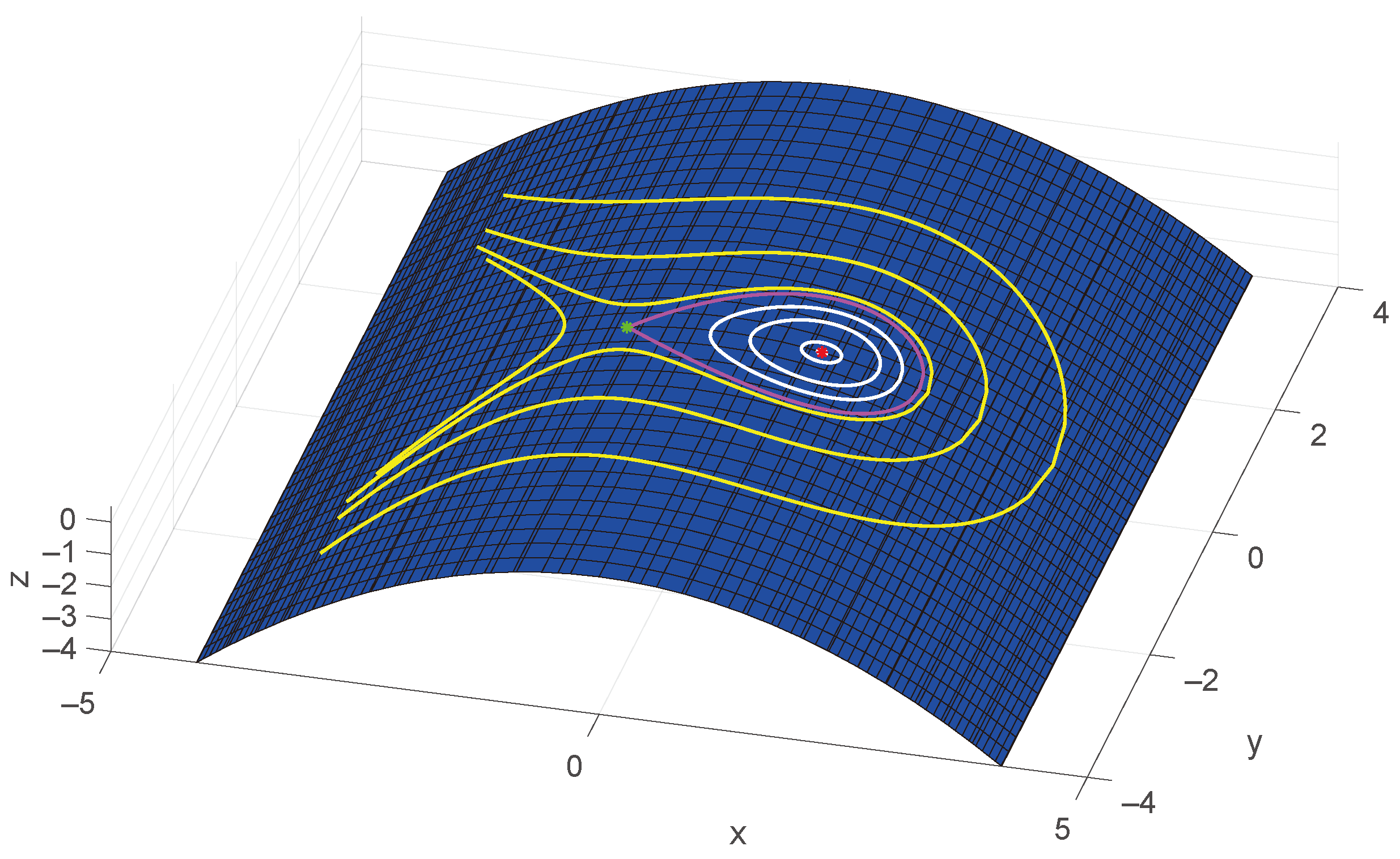
As a particular case, we consider $n=2$, that is,

$$\left\{\begin{array}{c}\dot{x}=y\hfill \\ \dot{y}=z\hfill \\ \dot{z}=-2\delta xy\hfill \end{array}\right..$$

(31)

Let $\delta >0$. Thus, the equilibrium point $e_M=(M,0,0),M>0$ is nonlinearly stable, and a family of periodic orbits of the above system surrounds it (white curves in Figure 1). Choosing initial conditions farther and farther from $e_M$, these periodic orbits approach the unstable equilibrium point $e_{-M},$ that is, they tend towards the homoclinic orbit that connects the unstable equilibrium point $e_{-M}$ with itself (the pink curve in Figure 1). After that, the unbounded curves appear in the dynamics of system (31) (yellow curves in Figure 1).

Figure 1. The dynamics of system (31) on the level set $C(x,y,z)=C(M,0,0)$ ($\delta =0.25; M=1$): periodic orbits (white) around the stable equilibrium point $(M,0,0), M>0$ (red), a homoclinic orbit (pink) that connects the unstable equilibrium point $(-M,0,0)$ (green) with itself, and unbounded curves (yellow).

Below, we deduce the parametric representation of the homoclinic orbit of system (31) in the case $\delta >0$ and $M<0$. Using (25) and (30), system (31) reduces to the equation

$$\dot{x}=\pm \sqrt{{\displaystyle \frac{2\delta }{3}}{(x-M)}^2(-2M-x)}.$$

By integration and (25), (31), we obtain the homoclinic orbit

$${\mathcal{H}}_M^{-}:\mathbb{R}\to {\mathbb{R}}^3,{\mathcal{H}}_M^{-}\left(t\right)=(x\left(t\right),y\left(t\right),z\left(t\right)),$$

where

$$\begin{array}{cc}\hfill x\left(t\right)& =\frac{432M^3}{{\left(e^{(t-t_0)\sqrt{-2\delta M}}-6M\right)}^2}+\frac{72M^2}{e^{(t-t_0)\sqrt{-2\delta M}}-6M}+M,\hfill \\ \hfill y\left(t\right)& =-\frac{72\sqrt{-2\delta M}\left(M^2{e}^{(t-t_0)\sqrt{-2\delta M}}\left(e^{(t-t_0)\sqrt{-2\delta M}}+6M\right)\right)}{{\left(e^{(t-t_0)\sqrt{-2\delta M}}-6M\right)}^3},\hfill \\ \hfill z\left(t\right)& =-\delta M^2\left[\frac{{\left(60M{e}^{(t-t_0)\sqrt{-2\delta M}}+e^{2(t-t_0)\sqrt{-2\delta M}}+36M^2\right)}^2}{{\left(e^{(t-t_0)\sqrt{-2\delta M}}-6M\right)}^4}-1\right],\hfill \end{array}$$

where $t_0$ is an arbitrary constant.

A similar result is obtained in the case $\delta <0$ ($M>0$), namely, the homoclinic orbit

$${\mathcal{H}}_M^{+}:\mathbb{R}\to {\mathbb{R}}^3,{\mathcal{H}}_M^{+}\left(t\right)=(x\left(t\right),y\left(t\right),z\left(t\right)),$$

where

$$\begin{array}{cc}\hfill x\left(t\right)& =\frac{432M^3}{{\left(e^{(t-t_0)\sqrt{-2\delta M}}+6M\right)}^2}-\frac{72M^2}{e^{(t-t_0)\sqrt{-2\delta M}}+6M}+M,\hfill \\ \hfill y\left(t\right)& =\frac{72\sqrt{-2\delta M}\left(M^2{e}^{(t-t_0)\sqrt{-2\delta M}}\left(e^{(t-t_0)\sqrt{-2\delta M}}-6M\right)\right)}{{\left(e^{(t-t_0)\sqrt{-2\delta M}}+6M\right)}^3},\hfill \\ \hfill z\left(t\right)& =\frac{144\delta M^3{e}^{(t-t_0)\sqrt{-2\delta M}}\left(-24M{e}^{(t-t_0)\sqrt{-2\delta M}}+e^{2(t-t_0)\sqrt{-2\delta M}}+36M^2\right)}{{\left(e^{(t-t_0)\sqrt{-2\delta M}}+6M\right)}^4}.\hfill \end{array}$$

5. Conclusions

In this paper, we constructed a family of Hamilton–Poisson jerk systems and we studied some dynamical properties.

The dynamics of a three-dimensional Hamilton–Poisson system take place at the intersection of the level sets given by the two constants of motion. Thus, for particular constants of motion, the orbits of the system can be depicted. In general, we studied the stability of the equilibrium points, and we proved the existence of periodic orbits around nonlinearly stable equilibrium points. Also, we established conditions for the existence of homoclinic and heteroclinic orbits. Particularly, we applied the results to a family of anharmonic oscillators.

We noticed that jerk versions of some nonlinear oscillators belong to this family, particularly the harmonic oscillator and some anharmonic oscillators. In quantum field theory (QFT), while the harmonic oscillator is a fundamental concept, there are other general potentials, including anharmonic potentials. Consequently, we expect some connections between our work and QFT, particularly solitons.