
The Efficiency of Hazard Rate Preservation Method for Generating Discrete Rayleigh–Lindley Distribution


Abstract
1. Introduction
- The survival discretization method: The advantage of employing the survival discretization technique lies in its ability to preserve the statistical characteristics of the basic distribution, such as the median and percentiles, alongside the distribution’s general shape. However, a limitation of this approach is its computational demand, often necessitating the use of numerical methods to handle complicated distributions.
- The hazard rate preservation method: This technique is designed to maintain the hazard function’s structure when transitioning from a continuous to a discrete setting. The hazard function, which represents the instant rate of failure at any given time, is crucial for understanding the likelihood of an event occurring at a specific moment, provided the event has not yet occurred. One of the primary benefits of this method is its ability to closely replicate the behavior of the original continuous distribution in a discrete framework. This is particularly valuable in reliability engineering and survival analysis, where the timing of events is critical. A limitation of this approach is that it may require substantial computational resources, especially for complex distributions or when high precision is needed. This may limit its applicability in real-time or resource-constrained environments.
2. Rayleigh–Lindley Distribution and Methods of Discretization
2.1. The Method of Survival Discretization
- Effect of : As the value of increases, the pmf curves tend to flatten, indicating a broader spread of the probabilities across different values of k. This suggests that a larger parameter will reduce the rate at which probabilities decay, leading to a more uniform distribution of the probability mass over the range of k. It highlights ’s role in controlling the dispersion of the distribution.
- Effect of : The parameter affects the shape and skewness of the pmf curves. For a fixed , varying alters how quickly the probabilities decrease as k increases. Higher values of tend to produce curves that drop off more sharply. This effect might be due to the exponential terms involving in the function, affecting the exponential decay rate of the pmf.
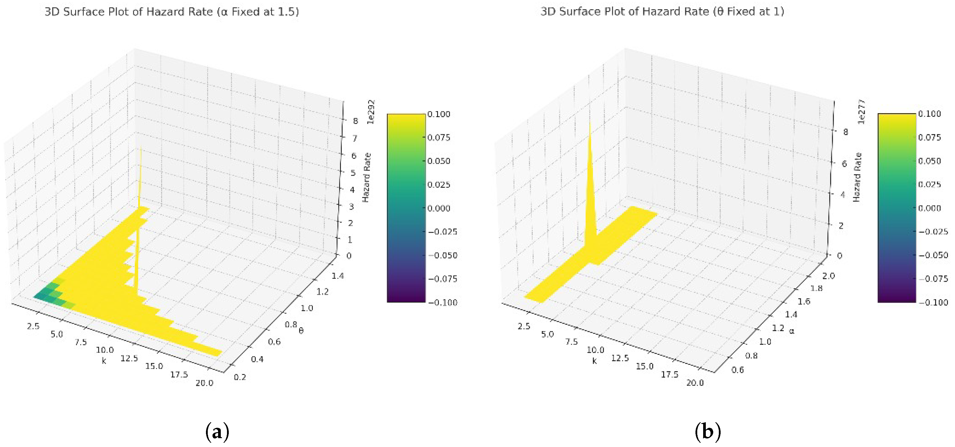
- Hazard rate with : With a fixed , the increasing values of tend to modulate the hazard rate’s sensitivity to changes in k. Specifically, lower values of yield steeper curves, indicating a higher hazard rate change rate over k. Conversely, higher values result in more gradual curves, suggesting a slower change in the hazard rate over k. This style highlights ’s influence on spreading the risk over time, with higher values smoothing the rate of change in the hazard rate.
- Hazard rate with : Keeping constant, the variation in values reveals distinct trends in the hazard rate’s evolution. Lower values produce relatively flat curves, indicating a more uniform hazard rate across k. As increases, the curves show a sharper descent, underscoring a rapid decrease in the hazard rate after an initial peak. This behavior showcases ’s role in determining the hazard rate’s peak and subsequent decline, with higher values accelerating the peak’s onset.
2.2. Hazard Preservation Method
- As k increases from 1 onwards, the probability shows a decreasing trend for all combinations of and . However, the rate of decrease and the pattern of the probabilities vary significantly with different values of and . This variation illustrates how these parameters modulate the distribution, affecting both the likelihood of higher k values and the distribution’s tail.
- The decay pattern of as k increases suggests that the distribution’s tail becomes thinner or heavier depending on the values of and . For some parameter combinations, the probability decreases more sharply, indicating a thinner tail. In contrast, other combinations show a more gradual decrease, suggesting a heavier tail and hence a higher probability of larger k values.
- Comparing curves of different colors (each representing a unique combination of and ) indicates that higher values of and/or generally result in a quicker drop-off in the probability as k increases. This suggests that larger values of these parameters make higher k values less likely, potentially due to the increased spread or dispersion introduced by and the rate of decrease in probability mass with k influenced by .
- The product term in the pmf for k > 0 accumulates the effect of all previous k values, introducing a dependence that shapes the overall distribution. The gradual decrease for k > 1 highlights the cumulative impact of preceding probabilities, emphasizing the distribution’s memory of past values. This effect is particularly noticeable in distributions where the probabilities do not drop to near-zero immediately, illustrating the balance between the likelihood of consecutive events.
3. Statistical Functions
3.1. Quantile Function
3.2. Moments
3.3. Order Statistics
4. Maximum Likelihood Estimation
5. Bayesian Inference
- (i)
- Squared error (SE) loss function: assuming SE loss function, Bayes estimation for the parameters and are defined as the mean or expected value for the joint posterior
- (ii)
- LINEX loss function: under LINEX loss function, estimating parameters with Bayesian method is written aswhere h is the value of the shape factor and it represents the orientation of asymmetry; hence, in our study we select the values of h to be 1.5 and −1.5 in the simulation analysis.
6. Simulation Analysis
- It is evident that the estimated parameter values approach the true values as the sample size increases. This is indicated by the reduction in both MSE and bias with larger sample sizes, demonstrating the consistency of the proposed estimators.
- When working with small sample sizes, Bayesian estimation with LINEX loss function yields the lowest MSE and bias for estimating the parameter . In contrast, the SE loss function produces the smallest MSE and bias for estimating .
- For big sample sizes, LINEX loss function consistently achieves the lowest MSE and bias for the two parameters and .
- For both parameters and , the Bayesian methods generally show a different bias and MSE pattern compared to MLE. Specifically, the Bayesian SE method tends to have lower MSE than MLE in many cases, suggesting that it might provide more accurate and reliable estimates under certain conditions. For nearly all scenarios, both the LINEX and SE loss functions result in the lowest bias and MSE values across various sample sizes.
- The LINEX penalties introduce variability in the performance, with LINEX-1.5 generally resulting in higher bias and MSE for , especially when , suggesting a sensitivity to the loss function’s shape.
- The performance of the estimation methods varies significantly between the two parameter settings and = 0.5 vs. 2. For instance when and are both set to 2, the bias and MSE are generally higher compared to when they are set to 0.5. This suggests that the true values of the parameters can significantly affect the difficulty of the estimation problem.
- Across both distributions, the Bayesian methods, particularly with the Standard Error (SE) approach, often show a lower MSE compared to the MLE, suggesting that in the context of these simulations, Bayesian methods might offer a more robust approach under certain conditions.
- The bias for parameter in DRLD2 seems to have less variability across different methods and conditions compared to DRLD1. For example, in DRLD2, the bias values for are generally closer to zero, especially in the Bayesian SE and LINEX (−1.5) scenarios, indicating potentially more accurate estimations. For parameter , the bias is also generally lower in DRLD2, suggesting that the estimation methods may perform better on this distribution for .
- The MSE values for both and tend to be lower in DRLD2 across most methods and conditions, indicating a more precise estimation. This is particularly evident in the Bayesian SE and LINEX (−1.5) methods, where the improvement in MSE is clear.
- The impact of increasing sample size on improving bias and MSE appears to be more consistent in DRLD2 than in DRLD1, especially for the Bayesian methods. This suggests that DRLD2 may be more amenable to these estimation techniques as the sample size increases.
- The Bayesian methods, especially with SE and LINEX (−1.5), show a notable improvement in DRLD2 over DRLD1 in terms of both bias and MSE. This could be indicative of the Bayesian methods being particularly well-suited for the characteristics of DRLD2.
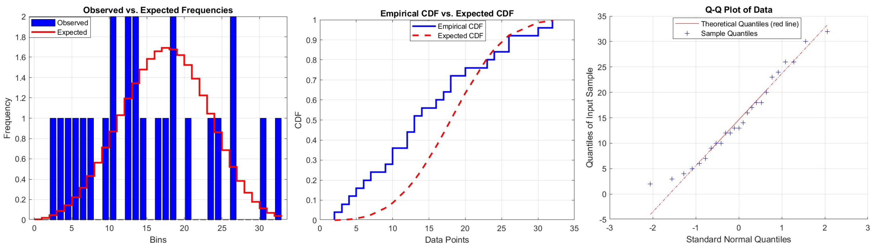
7. Real Data Examples
8. Conclusions
Funding
Data Availability Statement
Conflicts of Interest
References
- Xekalaki, E. Hazard function and life distributions in discrete time. Commun. Stat. Theory Methods 1983, 12, 2503–2509. [Google Scholar] [CrossRef]
- Roy, D.; Ghosh, T. A new discretization approach with application in reliability estimation. IEEE. Trans. Reliab. 2009, 58, 456–461. [Google Scholar] [CrossRef]
- Bracquemond, C.; Gaudoin, O. A survey on discrete life time distributions. Int. J. Reliabil. Qual. Saf. Eng. 2003, 10, 69–98. [Google Scholar] [CrossRef]
- Lai, C.D. Issues concerning constructions of discrete lifetime models. Qual. Technol. Quant. Manag. 2013, 10, 251–262. [Google Scholar] [CrossRef]
- Chakraborty, S. Generating discrete analogues of continuous probability distributions—A survey of methods and constructions. J. Stat. Distrib. Appl. 2015, 2, 6. [Google Scholar] [CrossRef]
- Roy, D. The discrete normal distribution. Commun. Stat. Theor. Methods 2003, 32, 1871–1883. [Google Scholar] [CrossRef]
- Roy, D. Discrete Rayleigh distribution. IEEE. Trans. Reliab. 2004, 53, 255–260. [Google Scholar] [CrossRef]
- Al-Huniti, A.A.; Al-Dayjan, G.R. Discrete Burr type III distribution. Am. J. Math. Stat. 2012, 2, 145–152. [Google Scholar] [CrossRef]
- Bebbington, M.; Lai, C.D.; Wellington, M.; Zitikis, R. The discrete additive Weibull distribution: A bathtub-shaped hazard for discontinuous failure data. Reliab. Eng. Syst. Saf. 2012, 106, 37–44. [Google Scholar] [CrossRef]
- Barbiero, A.; Hitaj, A. Discrete half-logistic distributions with applications in reliability and risk analysis. Ann. Oper. Res. 2024, 1–31. [Google Scholar] [CrossRef]
- Sarhan, A.M. A two-parameter discrete distribution with a bathtub hazard shape. Commun. Stat. Appl. Methods 2017, 24, 15–27. [Google Scholar] [CrossRef][Green Version]
- Yari, G.; Tondpour, Z. Discrete Burr XII-Gamma Distributions: Properties and Parameter Estimations. Iran. J. Sci. Technol. Trans. Sci. 2017, 42, 2237–2249. [Google Scholar] [CrossRef]
- Almetwally, E.M.; Ibrahim, G.M. Discrete Alpha Power Inverse Lomax Distribution with Application of COVID-19 Data. Int. J. Appl. Math. 2020, 9, 11–22. [Google Scholar]
- Eliwa, M.S.; Altun, E.; El-Dawoody, M.; El-Morshedy, M. A new three-parameter discrete distribution with associated INAR process and applications. IEEE Access 2020, 8, 91150–91162. [Google Scholar] [CrossRef]
- Al-Babtain, A.; Hadi, A.; Ahmed, N.; Afify, A.Z. A New Discrete Analog of the Continuous Lindley Distribution, with Reliability Applications. Entropy 2020, 22, 603. [Google Scholar] [CrossRef] [PubMed]
- Eldeeb, A.S.; Ahsan-Ul-Haq, M.; Babar, A. A Discrete Analog of Inverted Topp-Leone Distribution: Properties, Estimation and Applications. Int. J. Anal. Appl. 2021, 19, 695–708. [Google Scholar]
- Haj Ahmad, H.; Ramadan, D.A.; Almetwally, E.M. Evaluating the Discrete Generalized Rayleigh Distribution: Statistical Inferences and Applications to Real Data Analysis. Mathematics 2024, 12, 183. [Google Scholar] [CrossRef]
- Ahmad, H.H.; Almetwally, E.M. Generating optimal discrete analogue of the generalized Pareto distribution under Bayesian inference with application. Symmetry 2022, 14, 1457. [Google Scholar] [CrossRef]
- Haj Ahmad, H.; Bdair, O.M.; Naser, M.F.M.; Asgharzadeh, A. The rayleigh lindley distribution: A new generalization of rayleigh distribution with physical applications. Rev. Investig. Oper. 2023, 44, 1–18. [Google Scholar]
- Arnold, B.C.; Press, S.J. Compatible Conditional Distributions. J. Am. Stat. Assoc. 1989, 84, 152. [Google Scholar] [CrossRef]
- Karandikar, R.L. On the markov chain monte carlo (MCMC) method. Sadhana 2006, 31, 81–104. [Google Scholar] [CrossRef]
- Karlis, D.; Xekalaki, E.; Lipitakis, E.A. On some discrete valued time series models based on mixtures and thinning. In Proceedings of the Fifth Hellenic-European Conference on Computer Mathematics and Its Applications, Athens, Greece, 20–22 September 2001; pp. 872–877. [Google Scholar]
- Worldometers. Available online: https://www.worldometers.info/coronavirus (accessed on 1 June 2021).


| () | Median | Mean | Variance | Skewness | Kurtosis | Range | ||
|---|---|---|---|---|---|---|---|---|
| (0.30, 0.80) | 0.00 | 0.00 | 0.00 | 0.1906 | 0.1543 | 1.5755 | 3.4821 | 0–1 |
| (1.50, 0.50) | 2.00 | 3.00 | 4.00 | 3.0135 | 1.1724 | −0.3520 | 2.8274 | 0–6 |
| (1.00, 0.50) | 2.00 | 2.00 | 3.00 | 2.3541 | 0.8954 | −0.2713 | 2.7926 | 0–5 |
| (0.20, 0.40) | 0.00 | 1.00 | 1.00 | 0.8416 | 0.3669 | 0.0978 | 2.6259 | 0–3 |
| (0.60, 0.60) | 1.00 | 1.00 | 2.00 | 1.2112 | 0.4552 | −0.0750 | 2.5224 | 0–3 |
| () | Median | Mean | Variance | Skewness | Kurtosis | Range | ||
|---|---|---|---|---|---|---|---|---|
| (0.30, 0.80) | 0.00 | 1.00 | 2.00 | 1.25 | 3.58 | 2.29 | 9.67 | 0–15 |
| (1.50, 0.50) | 0.00 | 1.00 | 1.00 | 0.51 | 0.27 | 0.16 | 1.59 | 0–3 |
| (1.00, 0.50) | 0.00 | 0.00 | 1.00 | 0.51 | 0.29 | 0.76 | 7.56 | 0–7 |
| (0.20, 0.40) | 0.00 | 1.00 | 1.00 | 0.82 | 1.80 | 3.58 | 21.75 | 0–16 |
| (2.00, 3.00) | 0.00 | 1.00 | 2.00 | 1.36 | 3.91 | 2.14 | 9.18 | 0–17 |
| (3.50, 0.50) | 0.00 | 1.00 | 1.00 | 0.51 | 0.25 | −0.01 | 1.07 | 0–2 |
| (4.00, 0.50) | 0.00 | 1.00 | 1.00 | 0.50 | 0.25 | 0.01 | 1.06 | 0–2 |
| MLE | Bayes (SE) | Bayes (LINEX-1.5) | Bayes (LINEX 1.5) | ||||||||
|---|---|---|---|---|---|---|---|---|---|---|---|
| n | Bias | MSE | Bias | MSE | Bias | MSE | Bias | MSE | |||
| 0.5 | 0.5 | 50 | 0.2767 | 0.2983 | 0.3212 | 0.2058 | 0.4068 | 0.3078 | 0.2397 | 0.1283 | |
| 0.0082 | 0.0132 | 0.0124 | 0.0089 | 0.0207 | 0.0093 | 0.0392 | 0.0086 | ||||
| 100 | 0.2356 | 0.2307 | 0.1285 | 0.0419 | 0.1434 | 0.0487 | 0.1136 | 0.0359 | |||
| 0.0363 | 0.0107 | −0.0113 | 0.0045 | −0.0183 | 0.0044 | −0.0338 | 0.0046 | ||||
| 150 | 0.3009 | 0.0997 | 0.0808 | 0.0182 | 0.0866 | 0.0197 | 0.0751 | 0.0167 | |||
| 0.0337 | 0.0020 | −0.0104 | 0.0038 | −0.0144 | 0.0037 | −0.0246 | 0.0038 | ||||
| 2 | 50 | 0.5566 | 0.3608 | 0.5221 | 0.5461 | 0.6359 | 0.7618 | 0.4130 | 0.3687 | ||
| −0.3494 | 0.1234 | −0.4743 | 0.3857 | −0.4029 | 0.3057 | −0.5439 | 0.4715 | ||||
| 100 | 0.5084 | 0.3463 | 0.4526 | 0.2419 | 0.4738 | 0.2654 | 0.4059 | 0.2168 | |||
| −0.3299 | 0.1133 | −0.3927 | 0.1791 | −0.3753 | 0.1629 | −0.4083 | 0.1943 | ||||
| 150 | 0.4642 | 0.3350 | 0.4105 | 0.1794 | 0.4233 | 0.1915 | 0.3955 | 0.1657 | |||
| −0.3048 | 0.1024 | −0.3731 | 0.1465 | −0.3596 | 0.1355 | −0.3847 | 0.1562 | ||||
| 2 | 0.5 | 50 | 0.0949 | 0.0189 | 0.1408 | 0.2011 | 0.2307 | 0.2592 | 0.0498 | 0.1630 | |
| −0.0359 | 0.0015 | −0.0340 | 0.0024 | −0.0332 | 0.0024 | −0.0349 | 0.0025 | ||||
| 100 | 0.0936 | 0.0175 | 0.0366 | 0.0458 | 0.0540 | 0.0493 | 0.0193 | 0.0432 | |||
| −0.0325 | 0.0012 | −0.0328 | 0.0018 | −0.0308 | 0.0018 | −0.0328 | 0.0018 | ||||
| 150 | 0.0828 | 0.0162 | 0.0199 | 0.0170 | 0.0263 | 0.0177 | 0.0135 | 0.0165 | |||
| −0.0276 | 0.0011 | −0.0309 | 0.0017 | −0.0302 | 0.0017 | −0.0309 | 0.0017 | ||||
| 2 | 50 | 0.4530 | 0.3211 | 0.3866 | 0.4378 | 0.5541 | 0.6896 | 0.2218 | 0.2658 | ||
| −0.1637 | 0.0295 | −0.1801 | 0.0399 | −0.1737 | 0.0376 | −0.1866 | 0.0422 | ||||
| 100 | 0.3739 | 0.3020 | 0.1408 | 0.0698 | 0.1632 | 0.0806 | 0.1182 | 0.0603 | |||
| −0.1179 | 0.0215 | −0.1206 | 0.0344 | −0.1520 | 0.0335 | −0.1721 | 0.0415 | ||||
| 150 | 0.2530 | 0.2695 | 0.0899 | 0.0274 | 0.0982 | 0.0298 | 0.0815 | 0.0251 | |||
| −0.1195 | 0.0176 | −0.1209 | 0.0314 | −0.1421 | 0.0308 | −0.1621 | 0.0405 | ||||
| MLE | Bayes (SE) | Bayes (LINEX-1.5) | Bayes (LINEX 1.5) | ||||||||
|---|---|---|---|---|---|---|---|---|---|---|---|
| n | Bias | MSE | Bias | MSE | Bias | MSE | Bias | MSE | |||
| 0.5 | 0.5 | 50 | 0.2661 | 0.2635 | 0.3323 | 0.2177 | 0.4237 | 0.3308 | 0.2455 | 0.1332 | |
| 0.0026 | 0.0145 | 0.0151 | 0.0089 | 0.0236 | 0.0094 | 0.0063 | 0.0085 | ||||
| 100 | 0.2373 | 0.2410 | 0.1272 | 0.0432 | 0.1426 | 0.0501 | 0.1119 | 0.0371 | |||
| 0.0377 | 0.0125 | −0.0133 | 0.0048 | −0.0131 | 0.0047 | −0.0054 | 0.0050 | ||||
| 150 | 0.3020 | 0.0999 | 0.0801 | 0.0185 | 0.0860 | 0.0201 | 0.0742 | 0.0169 | |||
| 0.0339 | 0.0020 | −0.0125 | 0.0020 | −0.0114 | 0.0038 | −0.0046 | 0.0040 | ||||
| 2 | 50 | 0.5574 | 0.3163 | 0.4552 | 0.2611 | 0.4168 | 0.1873 | 0.2431 | 0.1400 | ||
| −0.3524 | 0.1254 | −0.3046 | 0.1185 | −0.2390 | 0.1031 | −0.2154 | 0.0947 | ||||
| 100 | 0.2587 | 0.2349 | 0.2426 | 0.2183 | 0.2045 | 0.1892 | 0.2040 | 0.1297 | |||
| −0.3340 | 0.1162 | −0.3042 | 0.1020 | −0.2402 | 0.1018 | −0.2044 | 0.0922 | ||||
| 150 | 0.1574 | 0.2035 | 0.1421 | 0.1750 | 0.1417 | 0.1486 | 0.1390 | 0.1136 | |||
| −0.3046 | 0.1023 | −0.2380 | 0.0915 | −0.1307 | 0.0901 | −0.0939 | 0.0816 | ||||
| 2 | 0.5 | 50 | 0.0541 | 0.0109 | −0.0601 | 0.0101 | 0.0914 | 0.0103 | −0.0666 | 0.0101 | |
| −0.0363 | 0.0015 | −0.0391 | 0.0013 | −0.0395 | 0.0013 | −0.0393 | 0.0013 | ||||
| 100 | 0.0496 | 0.0102 | 0.0479 | 0.0033 | −0.0536 | 0.0035 | −0.0564 | 0.0031 | |||
| −0.0330 | 0.0012 | −0.0361 | 0.0009 | −0.0390 | 0.0009 | −0.0385 | 0.0009 | ||||
| 150 | 0.0317 | 0.0092 | −0.0398 | 0.0014 | −0.0231 | 0.0014 | −0.0449 | 0.0013 | |||
| −0.0288 | 0.0012 | −0.0358 | 0.0008 | −0.0380 | 0.0008 | −0.0369 | 0.0009 | ||||
| 2 | 50 | 0.0541 | 0.0109 | 0.0431 | 0.0070 | 0.0555 | 0.0114 | 0.0305 | 0.0037 | ||
| −0.0363 | 0.0015 | −0.0215 | 0.0013 | −0.0206 | 0.0012 | −0.0223 | 0.0014 | ||||
| 100 | 0.0496 | 0.0102 | 0.0322 | 0.0014 | 0.0352 | 0.0017 | 0.0291 | 0.0012 | |||
| −0.0330 | 0.0012 | −0.0224 | 0.0012 | −0.0218 | 0.0011 | −0.0229 | 0.0012 | ||||
| 150 | 0.0317 | 0.0092 | 0.0214 | 0.0013 | 0.0225 | 0.0014 | 0.0201 | 0.0011 | |||
| −0.0288 | 0.0012 | −0.0244 | 0.0012 | −0.0234 | 0.0011 | −0.0252 | 0.0013 | ||||
| Parameters | MLE | p-Value | Test Statistics | |
|---|---|---|---|---|
| DRLD1 | 0.1684 | 0.8366 | 0 | |
| 0.0849 |
| Parameters | MLE | p-Value | Test Statistics | |
|---|---|---|---|---|
| DRLD2 | 0.1098 | 0.0853 | 0 | |
| 0.0305 |
Disclaimer/Publisher’s Note: The statements, opinions and data contained in all publications are solely those of the individual author(s) and contributor(s) and not of MDPI and/or the editor(s). MDPI and/or the editor(s) disclaim responsibility for any injury to people or property resulting from any ideas, methods, instructions or products referred to in the content. |
© 2024 by the author. Licensee MDPI, Basel, Switzerland. This article is an open access article distributed under the terms and conditions of the Creative Commons Attribution (CC BY) license (https://creativecommons.org/licenses/by/4.0/).
Share and Cite
Ahmad, H.H. The Efficiency of Hazard Rate Preservation Method for Generating Discrete Rayleigh–Lindley Distribution. Mathematics 2024, 12, 1261. https://doi.org/10.3390/math12081261
Ahmad HH. The Efficiency of Hazard Rate Preservation Method for Generating Discrete Rayleigh–Lindley Distribution. Mathematics. 2024; 12(8):1261. https://doi.org/10.3390/math12081261
Chicago/Turabian StyleAhmad, Hanan Haj. 2024. "The Efficiency of Hazard Rate Preservation Method for Generating Discrete Rayleigh–Lindley Distribution" Mathematics 12, no. 8: 1261. https://doi.org/10.3390/math12081261
APA StyleAhmad, H. H. (2024). The Efficiency of Hazard Rate Preservation Method for Generating Discrete Rayleigh–Lindley Distribution. Mathematics, 12(8), 1261. https://doi.org/10.3390/math12081261