Hybrid Model of Natural Time Series with Neural Network Component and Adaptive Nonlinear Scheme: Application for Anomaly Detection

Abstract

It is often difficult to describe natural time series due to implicit dependences and correlated noise. During anomalous natural processes, anomalous features appear in data. They have a nonstationary structure and do not allow us to apply traditional methods for time series modeling. In order to solve these problems, new models, adequately describing natural data, are required. A new hybrid model of a time series (HMTS) with a nonstationary structure is proposed in this paper. The HMTS has regular and anomalous components. The HMTS regular component is determined on the basis of an autoencoder neural network. To describe the HMTS anomalous component, an adaptive nonlinear approximating scheme (ANAS) is used on a wavelet basis. HMTS is considered in this investigation for the problem of neutron monitor data modeling and anomaly detection. Anomalies in neutron monitor data indicate negative factors in space weather. The timely detection of these factors is critically important. This investigation showed that the developed HMTS adequately describes neutron monitor data and has satisfactory results from the point of view of numeric performance. The MSE model values are close to 0 and errors are white Gaussian noise. In order to optimize the estimate of the HMTS anomalous component, the likelihood ratio test was applied. Moreover, the wavelet basis, giving the least losses during ANAS construction, was determined. Statistical modeling results showed that HMTS provides a high accuracy of anomaly detection. When the signal/noise ratio is 1.3 and anomaly durations are more than 60 counts, the probability of their detection is close to 90%. This is a high rate in the problem domain under consideration and provides solution reliability of the problem of anomaly detection in neutron monitor data. Moreover, the processing of data from several neutron monitor stations showed the high sensitivity of the HMTS. This shows the possibility to minimize the number of engaged stations, maintaining anomaly detection accuracy compared to the global survey method widely used in this field. This result is important as the continuous operation of neutron monitor stations is not always provided. Thus, the results show that the developed HMTS has the potential to address the problem of anomaly detection in neutron monitor data even when the number of operating stations is small. The proposed HMTS can help us to decrease the risks of the negative impact of space weather anomalies on human health and modern infrastructure.

1. Introduction

Information retrieval from natural data includes stages for the construction of models, methods and algorithms of analysis. The known problems in this field are nonstationary data and incomplete a priori knowledge on the information component and noise. This significantly complicates the process of model construction and methods for natural data analysis. In some critical related fields (physics and technique, biology, medicine, etc.), such a problem results in the insufficient efficiency of existing methods. This is of high significance regarding the problems of natural anomaly detection (earthquakes, space weather anomalies, tsunamis, etc.) [1].

The object of research in this paper is the data from global network neutron monitors recording intensity variations (particles per a minute) in cosmic rays (CRs). Neutron monitor data time series contain regular cyclic components (22-year, 11-year, 27-day and solar-diurnal variations) and anomalous features of nonstationary structures having the form of bursts of different amplitudes and durations, series of spikes, etc. [2]. Generation factors of such anomalies are coronal mass ejections (CMEs), high-speed solar wind streams from coronal holes and anomalous processes in the near-Earth space. Neutron monitor data anomalies indicate negative factors of space weather such as occurrences of Forbush effects (sudden decreases and/or increases in cosmic ray intensity) or GLE events (ground-level enhancement events—strong anomalous increases in cosmic ray intensity on the Earth’s surface) [3]. During such anomalies, radiation hazards for astronauts, airplane crews and passengers on polar routes increase. Space systems also undergo negative impacts due to technique losses. Thus, the near-real-time detection of anomalies in neutron monitor data is an important applied aspect of research [1].

The investigation of cosmic ray (CR) variations and the development of methods for their analysis began in the first half of the 20th century and has continued through today. One of the most successful and known methods for the investigation of CR parameters is the global survey method [4]. This method includes the method of CR variation communication functions, the method of particle trajectory calculations and spherical analysis for the detection of particle significant spherical harmonics [4]. The global survey method makes it possible to estimate CR flux characteristics with satisfactory accuracy in the case of an uninterrupted operation of a certain number of recording stations. However, due to calculation complexity, the method cannot be realized in automatic mode and it is not effective for the detection of initial proton increases.

Threshold algorithms, used by the Australian Space Weather Service [5] and GLE Alert system [6] to analyze CR variations, make short-term forecasts of radiation hazards according to the data of neutron monitors in an on-line regime. However, the efficiency of these algorithms is low due to their insensitivity to low-amplitude anomalies. The investigations in [7] showed that the GLE Alert algorithm can give unreliable results. Application of this algorithm for 3 years did not allow identification of more than 50% of solar proton events.

Thus, the applied methods for neutron monitor data analysis do not satisfy modern requirements and new approaches are needed in this field [8].

A high proportion of uncertainty in knowledge, the significant nonstationarity of neutron monitor data and noise correlation make it difficult to apply classical methods for time series analysis (ARIMA models, methods for time series decomposition, etc.) and result in low efficiency [9]. At the present time, methods of artificial intelligence and machine learning are actively applied in different applied fields to solve these problems. For example, the authors of [10,11] suggested using neural networks to forecast the state of oil pipelines. The approach in [10], based on the application of neural networks of direct propagation, made it possible to forecast the conditions of oil pipeline exploitation and to classify metal loss defects. In the research in [12], the authors proposed using neural networks with Bayesian regularization in order to solve this problem. A new approach was suggested in [12] to forecast the operation capability of a dry gas transmission system and to classify whether the amount of metal loss was effective even in the case of the absence of a priori data. For the problem of the diagnostics of rotating machine faults, a group of researchers [13] developed a model of a neural network with deep momentum transfer (SNN). The investigations in [13] showed that the developed method allows one to carry out contactless processing of visual data event fluxes, distinguish features and make diagnostics of machine faults.

In the field of this investigation, the author of [14] studied the possibility of application of graph neural networks to investigate the CR data energy spectrum. The neural network approach in [14] made it possible to decrease the time and computational efforts and showed more accurate results compared to the application of the likelihood function. However, the method results in [14] significantly depend on CR primary energy and on the configuration features of an applied detector.

The authors of [15] suggested a method for analysis of the arrival directions of super-high energy cosmic ray fluxes using a deep convolutional neural network. The results in [15] showed that the suggested method is more effective and more sensitive than the approach based on the angle power spectrum. The advantages of the method are the low generalization and efficiency decreases of the neural network when test models deviate from those used for training.

At the present time, hybrid models are actively developing to solve the problems indicated above. They combine classical statistical methods for data analysis and new developments in the fields of artificial intellect, machine learning and signal digital processing. The synthesis of mathematical techniques with adaptive modern tools allows one to extend the capabilities of applied constructs and to improve their efficiency [8,16,17,18,19,20,21,22]. For example, the paper [17] suggests a hybrid model based on the combination of the method of empirical mode decomposition (EMD) and the deep LSTM neural network. The approach proposed in [17] makes it possible to forecast the time series of climatic indexes and solar spots with long-term periodic behavior. The forecast changeability (or uncertainty) is suggested to be detected on the basis of the combination of the EMD method and the K-nearest neighbor. The paper [21] proposes an approach to the forecast of total electron content in the ionosphere (ionospheric parameter). This approach includes a combination of methods for ensemble empirical mode decomposition, K-averages and the self-service LSTM neural network. According to the estimates, the model suggested in [21] has a higher performance compared to some typical forecast methods applied to this problem. A hybrid model of a time series is suggested in [22]. It includes ARIMA components and multiple-scale wavelet analysis (MSA) components. The combination of the time series classical models with the MSA allowed one to obtain the adaptive model of an ionospheric parameters time series.

In this investigation, we propose a new hybrid model of a time series (HMTS) with nonstationary structure. It includes a neural network component and a nonlinear adaptive approximating scheme. The HMTS neural network component describes the data’s regular time variation and its parameters are estimated on the basis of an autoencoder network. The autoencoder is a nonlinear method of main components. It allows us to approximate dependences of a priori unknown structure and suppress noise. Today the autoencoder is successfully applied to solve different applied tasks. For example, in the paper [23] the authors suggested a federated semi-supervised method for the diagnostics of data transfer errors called targeted transfer learning through distribution barycenter medium (TTL-DBM). The application of the autoencoder network in [23] made it possible to aggregate key data distribution parameters and generate a distribution barycenter in an intermediate link for federated adaptation.

We applied the autoencoder network for the first time to approximate the regular time variation of neutron monitor data in the investigation in [24]. In the same paper [24] the autoencoder efficiency was shown for anomaly detection based on the search for the change points in a system. For the first time, we considered application of nonlinear approximating schemes for detection of anomalies in CR variations in [25]. The results in [25] showed the prospects of this approach for detection of multi-scale anomalies. Moreover, the possibility of application of both the autoencoder and the nonlinear approximating schemes was considered in the papers [24,25]. The investigations in [24,25] showed that the autoencoder is more effective for the detection of narrow-band anomalies, and the nonlinear approximating scheme is more effective for the detection of short-period different-scale anomalies. In the following research [26], we compared the method of singular spectral analysis (SSA) with the autoencoder and adaptive threshold filtering (AADA algorithm). The study [26] showed that the SSA can be applied to detect CR variation components during the process of dynamics analysis. However, the autoencoder and adaptive threshold wavelet filtering are more effective for anomaly detection. This paper continues these investigations. The combination of the autoencoder with the nonlinear approximating scheme in the form of the hybrid model of a time series with nonstationary structure develops that theory. This paper presents a formal form of the HMTS, and the methods to estimate its parameters have been developed. In order to optimize the calculation of the HMTS anomalous component, the likelihood ratio test was applied. The analytical expressions of threshold function parameters were obtained. They minimize data approximation errors. Moreover, the wavelet basis selection criterion, when constructing a nonlinear approximating scheme, was proposed. This allowed us to improve the HMTS efficiency for anomaly detection. Based on statistical modeling, the HMTS’s high efficiency was proved for the problem of anomaly detection in neutron monitor data.

2. Materials and Methods

2.1. Hybrid Model of a Natural Time Series of a Nonstationary Structure

A natural time series of a nonstationary structure can be represented in the following form:

$$f\left(t\right)=R\left(t\right)+A\left(t\right)+e\left(t\right)=\sum _r{S}_r\left(t,{\theta }_r\right)+\sum _{m}a\left[m\right]⟨f,g_m⟩g_m+e\left(t\right),$$

(1)

where $R\left(t\right)={\sum }_r{S}_r\left(t,{\theta }_r\right)$ is the regular component, which has a parametric form and is a linear combination of the components $S_r\left(t,{\theta }_r\right)$, $r$ is the component number, $\theta =\left\{{\theta }_r\right\}$ is the parameter set, $A\left(t\right)={\sum }_{m}a\left[m\right]⟨f,g_m⟩g_m$ is the nonstationary component, which includes local features of different forms and durations and is represented in the form of a nonlinear approximating scheme [27], in which $a\left[m\right]$ depends on $⟨f,g_m⟩$, $g_m$ is the orthonormal basis, $⟨·⟩$ is the scalar product, $t$ is the time.

2.2. Determination of the Regular Component $R\left(t\right)$ of Model (1)

The regular component $R\left(t\right)$ of model (1) includes implicit complex regularities. Thus, we represent it by means of the autoencoder neural network. The autoencoder is a nonlinear method of main components, and it makes it possible to determine the form of hidden regularities and estimate their parameters [28]. In terms of the autoencoder, we obtain the following estimate for the regular component $R\left(t\right)$ of model (1):

$$\widehat{R}\left(t\right)=\sum _r{S}_r\left(t,{\theta }_r\right)=Z\left({{\theta }_r}^{\left(2\right)}\left(H\left({{\theta }_r}^{\left(1\right)}f\left(t\right)\right)\right)\right),$$

(2)

where $Z$, $H$ are the activation functions of the neural network for output and inner layers, respectively, $\theta ={\left\{{{\theta }_r}^{\left(i\right)}\right\}}_{i=\mathrm{1,2}}$ are the parameters, ${{\theta }_r}^{\left(i\right)}$ are the weight matrix of the $i$-th layer.

From ratio (2) we estimate the parameters $\widehat{\theta }={\left\{{{\widehat{\theta }}_r}^{\left(i\right)}\right\}}_{i=\mathrm{1,2}}$ of model (1) based on minimizing the cost function [28].

$$C_{NET}=\sum _{k=1}^l{‖\widehat{R}\left(t\right)-f^{\left(k\right)}\left(t\right)‖}^2;\widehat{\theta }={argmin}_{\theta \in \Theta }\sum _{k=1}^l{‖\widehat{R}\left(t\right)-f^{\left(k\right)}\left(t\right)‖}^2,$$

(3)

where $f^{\left(k\right)}\left(t\right)$ is the $k$-th example (data sampling), $\Theta$ is the parameter set.

To verify the adequacy of the estimated regular component $\widehat{R}\left(t\right)$ (ratio (2)), for example, Ljung–Box $Q$-statistics can be applied [29]. The $Q$-statistics tests the hypothesis on the absence of model residuals’ autocorrelation. In order to test the normality of the model residuals’ distribution, the Jarque–Bera test can be used [29].

2.3. Determination of the Anomalous Component $A\left(t\right)$ of Model (1)

The anomalous component $A\left(t\right)$ of model (1) has a nonstationary structure and is represented in the form of the nonlinear approximating scheme (1).

$$A\left(t\right)=\sum _{m}a\left[m\right]⟨f,g_m⟩g_m,$$

(4)

where it is assumed that $f\in L^2\left(R\right)$, $L^2\left(R\right)$ is the Lebesgue space.

For nonparametric representation (4), the problem of estimation of the component $A\left(t\right)$ parameters is reduced to the filtering problem, which consists of the construction of the operator $D_A$ minimizing the risk:

$$\mathcal{R}\left(D_{A}f,A\right)=\underset{D_A\in O}{inf}E\left\{{‖D_{A}f-A‖}^2\right\},$$

(5)

where $E$ is the mathematical expectation, $‖·‖$ is the norm in $L^2\left(R\right)$, $O$ is the operator set.

In ratio (4), the nonlinear diagonal operator is considered as the operator $D_A$ [30], thus, risk (5) is determined by the following value [27]:

$$\mathcal{R}\left(D_{A}f,A\right)={\rm E}\left\{{‖\widehat{A}-A‖}^2\right\}=\sum _{m=1}^N{\rm E}\left\{{\left|⟨A,g_m⟩-⟨f,g_m⟩a\left[m\right]\right|}^2\right\},$$

(6)

$N$ is the series length.

Then, we assume that

$$f\left(t\right)=A\left(t\right)+e_A\left(t\right),$$

(7)

where the noise $e_A\left(t\right)$ is correlated and the noise coefficient dispersion ${\sigma }_m^2=E\left\{{\left|⟨e_A,g_m⟩\right|}^2\right\}$ depending on $g_m$, the mathematical expectation of noise $E\left\{e_A\left(t\right)\right\}=0$. Then, from ratio (7), the risk $\mathcal{R}\left(D_{A}f,A\right)$ (6) is minimum when [27]

$$a\left[m\right]=\frac{{\left|⟨A,g_m⟩\right|}^2}{{\left|⟨A,g_m⟩\right|}^2+{\sigma }_m^2}.$$

(8)

If we assume that $a\left[m\right]\in \left\{\mathrm{0,1}\right\}$, the operator $D_A$, minimizing the risk in (8), can be determined as [30]

$$a\left[m\right]=\left\{\begin{array}{c}1,if\left|⟨A,g_m⟩\right|\ge {h\times \sigma }_m\\ 0,if\left|⟨A,g_m⟩\right|<h\times {\sigma }_m\end{array}\right.,h=\sqrt{2lnN}.$$

(9)

Taking into account (9), the risk [30]

$${\mathcal{R}\left(D_{A}f,A\right)=\mathcal{R}}_{{\sigma }_m}\left(A\right)={\rm E}\left\{{‖D_{A}f-A‖}^2\right\}=\sum _{m=0}^{N}min\left({\left|⟨A,g_m⟩\right|}^2,{\sigma }_m^2\right).$$

(10)

Then, applying the threshold estimate in the orthonormal wavelet basis $G_{\Psi }={\left\{{\Psi }_{k,n}\right\}}_{\left(k,n\right)\in Z^2}$, ${\Psi }_{k,n}\left(t\right)=2^{\frac{k}{2}}\Psi \left(2^{k}t-n\right)$, the operator $D_{A_{\Psi }}$, minimizing the risk, is [31]

$$\widehat{A}\left(t\right)=D_{A_{\Psi }}f\left(t\right)=\sum _k\sum _{n=1}^N{P}_{{\sigma }_{k,n}}\left(⟨f,{\Psi }_{k,n}⟩\right){\Psi }_{k,n}\left(t\right),$$

(11)

where $P_{{\sigma }_{k,n}}\left(⟨f,{\Psi }_{k,n}⟩\right)=\left\{\begin{array}{c}⟨f,{\Psi }_{k,n}⟩,if\left|⟨f,{\Psi }_{k,n}⟩\right|\ge h^{\prime }\ast {\sigma }_{k,n}\\ 0,if\left|⟨f,{\Psi }_{k,n}⟩\right|<{h^{\prime }\ast \sigma }_{k,n}\end{array}\right.$,${\sigma }_{k,n}^2=E\left\{{\left|⟨e_{A_{\Psi }},{\Psi }_{k,n}⟩\right|}^2\right\}.$

The operator $D_{A_{\Psi }}$ in ratio (11) determines the nonlinear approximating scheme in the wavelet basis.

Note. In ratio (11) the threshold dependence $T_{k,n}=h^{\prime }\ast {\sigma }_{k,n}$ is considered both on the space variable $n$ (time) and on the scale $k$. This makes it possible to optimize the threshold both to time and scale changes of data. Moreover, as is shown below, in this case, thresholds close to optimal ones can be found based on the ratio criterion [32].

When joining the expression in (2) and (11), we obtain the hybrid model of a nonstationary time series (HMTS):

$$\begin{array}{c}f\left(t\right)=R\left(t\right)+A\left(t\right)+e\left(t\right)={\displaystyle \sum _r}{S}_r\left(t,{\theta }_r\right)+{\displaystyle \sum _m}a\left[m\right]⟨f,g_m⟩g_m+e\left(t\right)=\\ =Z\left({{\theta }_r}^{\left(2\right)}\left(H\left({{\theta }_r}^{\left(1\right)}f\left(t\right)\right)\right)\right)+{\sum }_k{\sum }_{n=1}^N{P}_{{\sigma }_{k,n}}\left(⟨f,{\Psi }_{k,n}⟩\right){\Psi }_{k,n}\left(t\right)+e\left(t\right),\end{array}$$

(12)

where $Z$ is the linear function of the network output layer activation, $H$ is the signoidal function of the network inner layer activation, $\theta ={\left\{{{\theta }_r}^{\left(i\right)}\right\}}_{i=\mathrm{1,2}}$ are the parameters of the neural network determined in ratio (3), $P_{{\sigma }_{k,n}}\left(·\right)$ is the threshold function with the thresholds determined in ratio (11).

2.4. Optimization of the HMTS. Determination of the Wavelet Basis Giving the Least Errors

From ratio (10), the risks of the estimates $\widehat{A}\left(t\right)$ on the wavelet basis can be limited by the value

$${\mathcal{R}}_{\Psi }\left(D_{A_{\Psi }}f,A\right)={\rm E}\left\{{‖D_{A_{\Psi }}f-A‖}^2\right\}=\sum _{k,n}min\left({\left|⟨A,{\Psi }_{k,n}⟩\right|}^2,{\sigma }_{k,n}^2\right)\le \sum _{k,n}{\sigma }_{k,n}^2.$$

(13)

Ratio (13) makes it possible to control the risk of the estimate $\widehat{A}\left(t\right)$ based on noise dispersion ${\sigma }_{k,n}^2$. Moreover, having estimated the risk for different bases from the dictionary $\Omega$ and using (13), we can determine the wavelet basis giving the least losses.

$${\Psi }^{op}: {\mathcal{R}}_{{\Psi }^{op}}\left(D_{A_{\Psi }}f,A\right)=\underset{\Psi \in \Omega }{\min }{\mathcal{R}}_{\Psi }\left(D_{A_{\Psi }}f,A\right).$$

(14)

2.5. Optimization of the Estimate of the Model Anomalous Component $\widehat{A}\left(t\right)$ by the Ratio Criterion

Derivation of an optimal estimate (10) is based on the assumption that $E\left\{e_A\left(t\right)\right\}=0$, which for the correlated noise ${\sigma }_m$ is not always realized. However, the function mapping into wavelet space gives an important advantage, which follows from the Jaffar theorem [27]: an increase in the amplitude of wavelet coefficients $\left|⟨f,{\Psi }_{k,n}⟩\right|$ indicates the appearance of a local feature of the function $f\left(t\right)$ in the vicinity of the point $t=n;$ out of the neighborhood, containing local features, wavelet coefficient amplitudes satisfy the condition

$$\left|⟨f,{\Psi }_{k,n}⟩\right|\le Q{k}^{q+0.5}= {П}_k,$$

(15)

$Q=const>0,$ $q$ is the Lipschitz index.

Thus, it follows from (15) that the values $\left|⟨f,{\Psi }_{k,n}⟩\right|=\left|⟨e_{A_{\Psi }},{\Psi }_{k,n}⟩\right|$ with respect to the argument $n$ are close to zero. Thus, the following condition is provided in the wavelet space: $E\left\{e_{A_{\Psi }}\left(t\right)\right\}=0$. The $\left|⟨f,{\Psi }_{k,n}⟩\right|=\left|c_{k,n}\right|$ value’s deviation from zero is the result of noise effect in this case (Figure 1).

Then, using the ratio criterion [32], we assume that there is a local feature in the vicinity of the point $t=n$ if

$$\frac{W\left(\left|c_{k,n}\right|{Г}_1\right)}{W\left(\left|c_{k,n}\right|{Г}_0\right)}\ge T_{k,n},$$

(16)

where $W\left(\left|c_{k,n}\right|{Г}_0\right)$ and $W\left(\left|c_{k,n}\right|{Г}_1\right)$ are the absolute value probability densities for the coefficients $\left|c_{k,n}\right|$ when a local feature is absent or is present, respectively. In its turn, following the Neyman–Pearson criterion [32], the threshold

$${T_{k,n}=T}_{\alpha ,k,n} (\alpha \mathrm{is\; the\; probability\; of} \mathit{I-}\mathrm{kind\; error})$$

(17)

is determined from the condition ${\int }_{\Phi }^{0}W\left(\left|c_{k,n}\right|{Г}_0\right)d\left|c_{k,n}\right|=\alpha ,$ where $\Phi$ is the critical region (Figure 1).

Thus, from (11), (16), (17) we obtain the optimized estimate of the model anomalous component in the form of the nonlinear adaptive approximating scheme (NAAS):

$$\widehat{A}\left(t\right)=D_{A_{\Psi }}f\left(t\right)=\sum _k\sum _{n=1}^N{P}_{T_{\alpha ,k,n}}\left(c_{k,n}\right){\Psi }_{k,n}^{op}\left(t\right),$$

(18)

where $P_{T_{\alpha ,k,n}}\left(c_{k,n}\right)=\left\{\begin{array}{c}{c}_{k,n},if\left|c_{k,n}\right|\ge T_{\alpha ,k,n}\\ 0,if\left|c_{k,n}\right|<T_{\alpha ,k,n}\end{array}\right.$, $T_{\alpha ,k,n}=t_{\frac{1-\alpha }{2}, M}{\widehat{\sigma }}_{k,n},$ $t_{\frac{1-\alpha }{2}, M}$ is the quantile of the level $\frac{1-\alpha }{2}$.

As the result, from (12), (18) we have the optimized hybrid model on a nonstationary time series (HMTS):

$$\begin{array}{c}f\left(t\right)=R\left(t\right)+A\left(t\right)+e\left(t\right)={\displaystyle \sum _r}{S}_r\left(t,{\theta }_r\right)+{\displaystyle \sum _m}a\left[m\right]⟨f,g_m⟩g_m+e\left(t\right)=\\ =Z\left({{\theta }_r}^{\left(2\right)}\left(H\left({{\theta }_r}^{\left(1\right)}f\left(t\right)\right)\right)\right)+{\displaystyle \sum _k}{\displaystyle \sum _{n=1}^N}{P}_{T_{\alpha ,k,n}}\left(c_{k,n}\right){\Psi }_{k,n}^{op}\left(t\right)+e\left(t\right),\end{array}$$

(19)

$Z$, $H$ are the activation functions, $\theta ={\left\{{{\theta }_r}^{\left(i\right)}\right\}}_{i=\mathrm{1,2}}$ are the model regular component parameters, $P_{T_{\alpha ,k,n}}\left(c_{k,n}\right)$ are the threshold functions with the thresholds $T_{\alpha ,k,n}=t_{\frac{1-\alpha }{2}, M}{\widehat{\sigma }}_{k,n}$, ${\Psi }_{k,n}^{op}\left(t\right)=2^{\frac{k}{2}}{\Psi }^{oп}\left(2^{k}t-n\right)$ is the wavelet.

3. Construction of the HMTS for Neutron Monitor Data

In the investigation, data from Nain, Inuvik, Oulu, Tule and South Pole stations were used [33]. The choice of the stations was determined by the experience of the experts from the applied subject field [4]. NM data record cosmic ray intensities (particles per minute). In the HMTS terms (representation (19)), NM data time variation can be represented as

$$f\left(t\right)=R\left(t\right)+A\left(t\right)+e\left(t\right)=Z\left({{\theta }_r}^{\left(2\right)}\left(H\left({{\theta }_r}^{\left(1\right)}f\left(t\right)\right)\right)\right)+\sum _k\sum _{n=1}^N{P}_{T_{\alpha ,k,n}}\left(c_{k,n}\right){\Psi }_{k,n}\left(t\right)+e\left(t\right),$$

(20)

where the regular cyclic component $R\left(t\right)=Z\left({{\theta }_r}^{\left(2\right)}\left(H\left({{\theta }_r}^{\left(1\right)}f\left(t\right)\right)\right)\right)$ includes periodicities of different amplitude and duration, shifts, spikes etc. (27-day and solar-diurnal, seasonal variations, etc.).

The nonstationary (anomalous) component $A\left(t\right)={\sum }_k{\sum }_{n=1}^N{P}_{T_{\alpha ,k,n}}\left(c_{k,n}\right){\Psi }_{k,n}\left(t\right)$ contains different-scale anomalous features in the form of bursts, spikes of different amplitude and duration, etc., which characterize the occurrences of Forbush effects and GLE events and are determined by anomalous processes on the Sun and in the near-Earth space; $e\left(t\right)$ is the noise.

The regular component of the NM data in the terms of the typical autoencoder neural network has the following form (see Formula (20)).

$$\widehat{R}\left(t\right)=Z\left({{\theta }_r}^{\left(2\right)}\left(H\left({{\theta }_r}^{\left(1\right)}f\left(t\right)+b^{\left(1\right)}\right)\right)+b^{\left(2\right)}\right),$$

(21)

where the upper index $\left(i\right)$ is the layer number, $H$ is the nonlinear activation function of the encoder (sigmoid), ${{\theta }_r}^{\left(1\right)}$ is the weight matrix of the network’s first layer, $Z$ is the linear activation function of the decoder (inner layer), ${{\theta }_r}^{\left(2\right)}$ is the weight matrix of the second layer, $b^{\left(i\right)}$ are the shift vectors.

Taking into account the local natural factor effect, neural networks for each station were trained separately. The neural networks were trained using the data from high-latitudinal and polar ground stations of neutron monitors. The network architecture for each station was typical [28] and included two layers. Taking into account data on diurnal variation, the network output vector length was 1440 counts (minute sampling). The network hidden layer length was determined empirically and was equal to 720 counts. The neural networks were trained on the basis of backpropagation, taking into account the application of a sparsity regularizer [28]. The training samples were formed from the neutron monitor data for 2013–2015 during the periods of absence of anomalous processes in the near-Earth space (calm periods). The calm periods were determined by the space weather data [34,35]. Solar and diurnal cycles were also taken into account during the selection.

Table 1. Estimate of the HMTS regular component $\widehat{R}\left(t\right)$ adequacy.

$\frac{1}{\mathit{N}}{\displaystyle \sum _{\mathit{t}=\overline{1,\mathit{N}}}}{\left(\mathit{f}\left(\mathit{t}\right)-\widehat{\mathit{R}}\left(\mathit{t}\right)\right)}^2$	Mean Squared Error
	High SA (2013–2015)	Low SA (2018–2020)
Inuvik st.	0.20418	0.17003
Nain st.	0.17231	0.15162
Tule st.	0.20212	0.16181
Oulu st.	0.19323	0.13104
South Pole st.	0.24245	0.19006

presents the results of the estimates of the model’s regular component $\widehat{R}\left(t\right)$ adequacy (Formula (21)). Data for the calm periods were used, and the mean squared error (MSE) was estimated. The results in Table 1 show that the MSE values are close to zero. We should note that the MSE during high solar activity (SA) significantly exceeded that during low solar activity. The highest MSE was obtained from the South Pole station data that is likely to be associated with its geographical location (the South Pole station is polar and the rest of the stations are high-latitudinal). The results from Table 1 confirm the adequacy of the estimated regular component $\widehat{R}\left(t\right)$ of the model.

The model’s $\widehat{R}\left(t\right)$ adequacy was verified using the Ljung–Box $Q$-statistics and the Jarque–Bera test [29]. The Ljung–Box $Q$-statistic ($Q_{stat}$) verifies the hypothesis on the joint equality of all the autocorrelations of the model residuals series up to the order $m$ inclusive. The Jarque–Bera fit test ($JB$) was applied to verify the normality of the model residuals’ distribution. The test results are illustrated in

Table 2. Results of the neural network performance.

	Results of a Network Trained on Data without Anomalies	Results of a Network Trained on Data without Anomalies	Results of a Network Trained on Data with Anomalies
NN input	Data without anomalies $JB=4.44;$ $Q_{stat}=54.75$;	Data with anomalies $JB=104.61;$ $Q_{stat}=3.85\times {10}^4$	Data with anomalies $JB=104.61;$ $Q_{stat}=3.85\times {10}^4$
NN output	$JB=2.77$; $Q_{stat}=3.2\times {10}^3;$	$JB=209.95$; $Q_{stat}=1.428\times {10}^4$	$JB=225.86;$ $Q_{stat}=2.11\times {10}^4$
NN errors	$JB=2.33;$ $Q_{stat}=30.23$	$JB=232.45;$ $Q_{stat}=8.836\times {10}^3$	$JB=68.64;$ $Q_{stat}=9.25\times {10}^4$

. The results in Table 1 indicate that the estimated model $\widehat{R}\left(t\right)$ adequately describes the NM data’s regular time variation, and the errors are the white Gaussian noise (column 1, Table 2). We should note that during the anomalies, the network errors significantly increase (column 2, Table 2). During the research, we also tried to train the network on the data containing anomalies (column 4, Table 2). However, due to the great diversity of anomaly forms, it is impossible to obtain an adequate model and to estimate its parameters. This fact confirms the necessity of taking into account the HMTS nonstationary (anomalous) component.

The anomalous component $A\left(t\right)$ parameters of the model were estimated using the NM data during the periods containing anomalous events in cosmic rays (Forbush effects) and observed during the disturbances in the near-Earth space (magnetic storms). The data were transformed by the discrete wavelet transform and threshold functions (see Formula (20)):

$$f\left(t\right)=\sum _{k=0}^K\sum _{n=1}^N{P}_{T_{\alpha ,k,n}}\left(c_{k,n}\right){\Psi }_{k,n}\left(t\right),$$

(22)

where ${\Psi }_{k,n}\left(t\right)=2^{\frac{k}{2}}\Psi \left(2^{k}t-n\right)$ are basic wavelets, $n, k\in N,c_{k,n}=⟨f\left(t\right),{\Psi }_{k,n}⟩$ are the coefficients of the $f\left(t\right)$ function’s decomposition into a series, $P_{T_{\alpha ,k,n}}\left(c_{k,n}\right)=\left\{\begin{array}{c}{c}_{k,n},if\left|c_{k,n}\right|\ge T_{\alpha ,k,n}\\ 0,if\left|c_{k,n}\right|<T_{\alpha ,k,n}\end{array}\right.$ is the threshold function, $N$ is the signal length, $K$ is the largest scale.

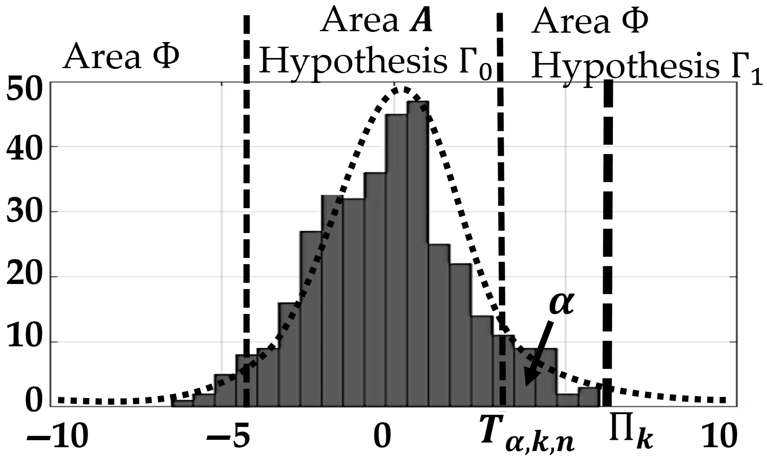
The thresholds $T_{\alpha ,k,n}=t_{\frac{1-\alpha }{2}, M}{\widehat{\sigma }}_{k,n}$ (Formula (22)) where determined with the significance level $\alpha =0.05$ (Neyman–Pearson criterion). The standard deviation ${\widehat{\sigma }}_{k,n}=\sqrt{\frac{1}{M}{\sum }_{n=1}^M{\left(c_{k,n}-\overline{c_{k,n}}\right)}^2}$ was estimated in the time window of the length $M=1440$ (determined by the solar-diurnal cycle). Orthonormal wavelets of Coiflets and Daubechies families were used as the basic wavelets.

Table 3. Estimates of the data approximation error using different wavelets.

${\displaystyle \sum _{\mathit{k},\mathit{n}}}{\mathit{\sigma }}_{\mathit{k},\mathit{n}}^2/‖\mathit{f}‖$		Wavelets
		coif_1	coif_2	coif_3	db_1	db_2
st. Inuvik	High SA	0.0175	0.0170	0.0176	0.0178	0.0174
	Low SA	0.0177	0.0175	0.0174	0.0178	0.0177
st. Oulu	High SA	0.0189	0.0187	0.0188	0.0190	0.0189
	Low SA	0.0202	0.0202	0.0201	0.0203	0.0200
Carrier size		6	12	18	2	4
Smoothness order		2	4	6	1	2

shows the results of the estimates of the NM data approximation errors using different wavelets (Formula (13)). The estimates show that the least error was obtained when using the Coiflet 2 and Daubechies 2 wavelets. When selecting the wavelet basis, the carrier size and the wavelet smoothness order were taken into consideration besides the errors. It is known [27] that the carrier size determines the vicinity dimensions containing the boundary effect. The smoothness order characterizes the capability of a wavelet to detect high-order features. Taking into account the wavelet properties indicated above, the Coiflet 2 wavelet was determined as the best one.

4. Application of the HMTS to Detect Anomalies

As illustrated above (column 2, Table 2), data time variation is disturbed during anomaly occurrences, and, as a consequence, modeling errors increase. Thus, detection of anomalies in NM data can be based on data modeling using the autoencoder (Formula (13)) and on the determination of the periods of neural network error increases. Then, to estimate anomaly parameters, the nonlinear approximating scheme on the wavelet basis was constructed (Formula (14)). The anomaly intensity was estimated from wavelet coefficient absolute values as

$$E_n=\sum _{k=0}^K{P}_{T_{\alpha ,k,n}}\left(c_{k,n}\right),$$

(23)

where $K=250$ is the largest scale analyzed.

The control-flow chart realizing the proposed method is illustrated in Figure 2.

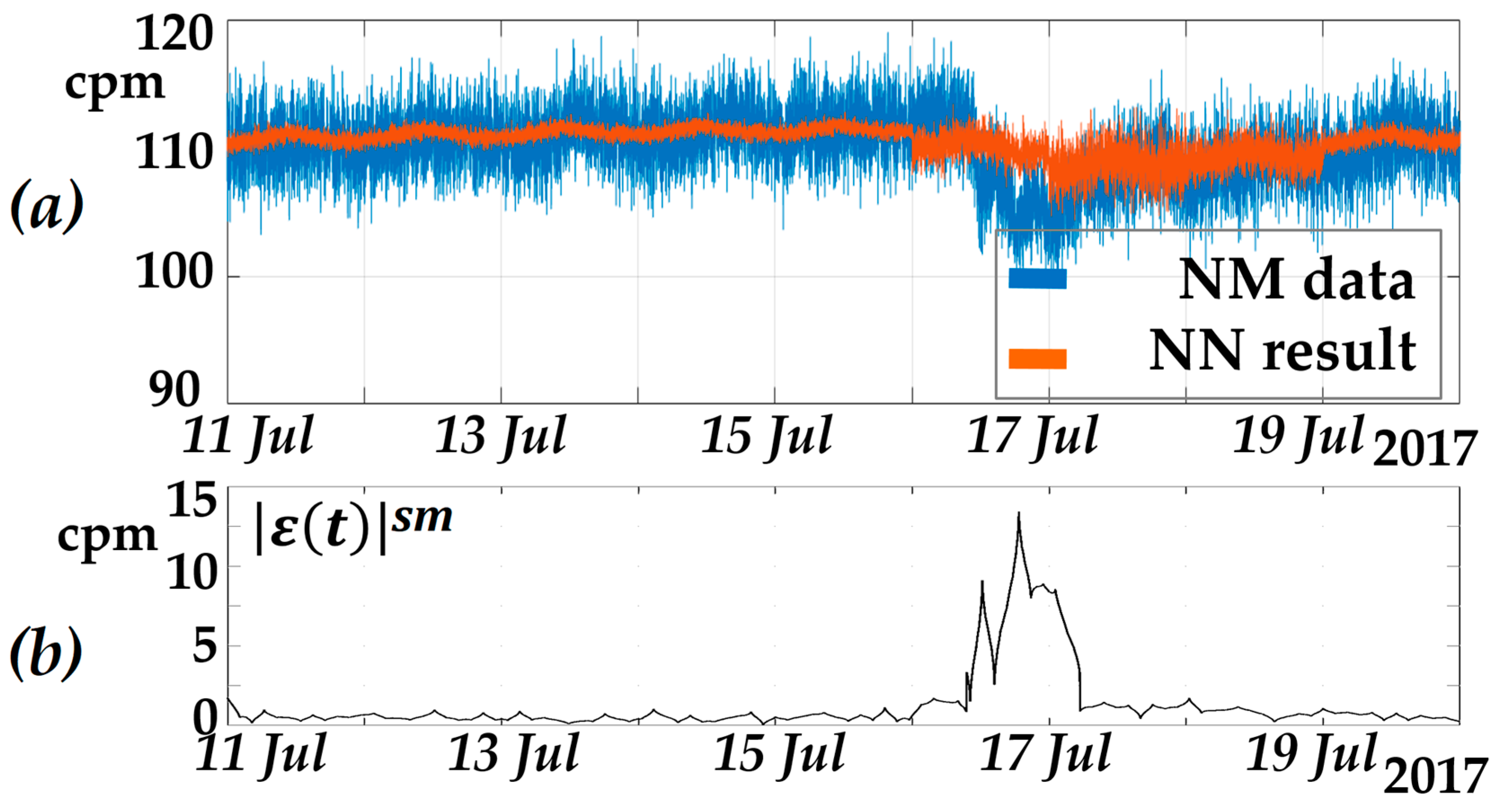
As an example, Figure 3 shows the results of the NM data modeling at Oulu station during an anomaly occurrence. Analysis of the results in Figure 3 shows the neural network error increase during the anomalous period that confirms the method’s efficiency.

The method’s efficiency was estimated using the neutron monitor data for 2013–2023. The data samples were formed for the periods containing the anomalies in cosmic ray variations (anomalous periods). The statistical modeling was performed. Both initial natural data and model data, formed on the basis of the natural data, were used in the estimates. The model data were formed using the wavelet packet operations [27] as follows:

(1) the data time series with the length of 1440 counts (diurnal variations) were formed, each count was equal to the corresponding median value of the neutron monitor’s initial data during calm periods;

(2) the obtained time series were decomposed into wavelet packets up to the 7th scale level (using Coiflet 1 wavelet; the 7th scale level was determined taking into account the series length);

(3) wavelet reconstruction of the time series’ smoothed components was carried out not taking into account the details ($X^{trend}$);

(4) local features of triangle-pulse form and the Gaussian-modeled pulse, which had different amplitude and duration ($X^{anom}$), were added to the obtained time series;

(5) additive correlated noise ($X^{noise}$) was added to the formed time series.

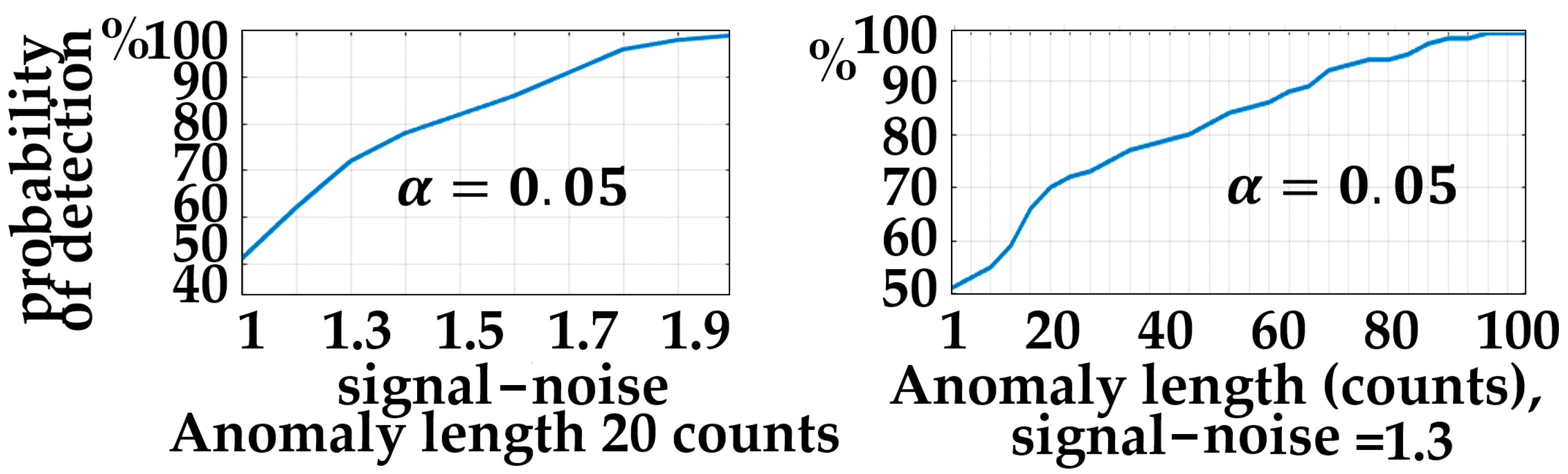
The graphs of anomaly detection probabilities, depending on anomaly amplitude (signal–noise ratio) and on anomaly duration, are illustrated in Figure 4. The analysis of the results shows that the detection probability for the anomaly, having the duration of 20 counts, is more than 80% for the signal–noise ratio of 1.5 (at the false alarm rate $\alpha =0.05$). When the anomaly is more than 60 counts, the detection probability is close to 90% for the signal–noise ratio of 1.3. The results show the high accuracy of the method.

Figure 5 shows the results of the detection of a low-amplitude anomaly (signal–noise ratio is 1.2) in the model signal against the background of correlated noise (pink noise was added). We should note that the anomaly in the noised model signal (Figure 5b) is not observed visually. The obtained result (Figure 5d) (see Formula (23)) confirms the high accuracy of the method for detection of anomalies including low-amplitude anomalies.

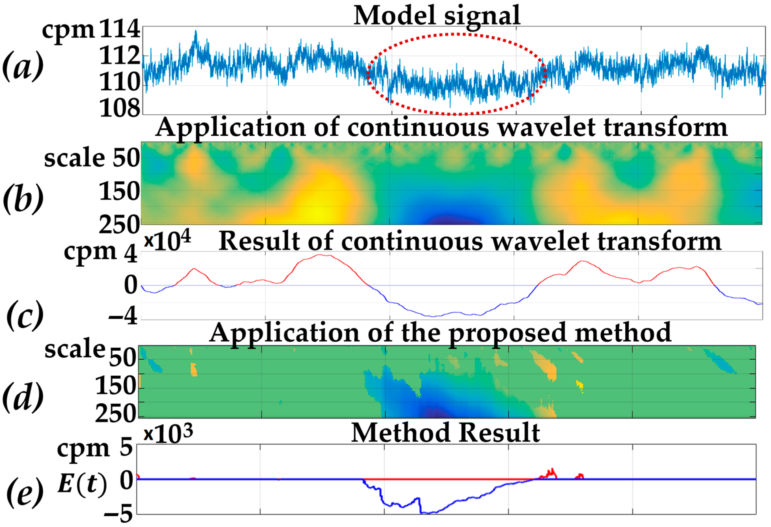
Figure 6 shows the results of the method (Figure 6d,e) on the model data with correlated (pink) noise (Figure 6b). In order to make the comparison, the results of application of a continuous wavelet transform (CWT) are illustrated (Figure 6c,d). The CWT results agree well with the method results. However, due to the correlated noise effect (including the solar-diurnal cycle), it is impossible to detect an anomaly in the data based on the CWT.

Figure 7 illustrates the results of the suggested method using the NM data from Oulu station (Figure 6a) and using the model data (Figure 7e). Based on the data [34], the Forbush effect was recorded at 05:59 UT on 16 July 2017. The magnetic storm [35] was recorded at Novosibirsk station at 06:00 UT on 17 July 2017. The period, containing anomalous changes, is marked by a red dashed-line oval. The results show that application of the suggested method makes it possible to detect anomalies both in natural (Figure 7c,d) and in model data (Figure 7g,h).

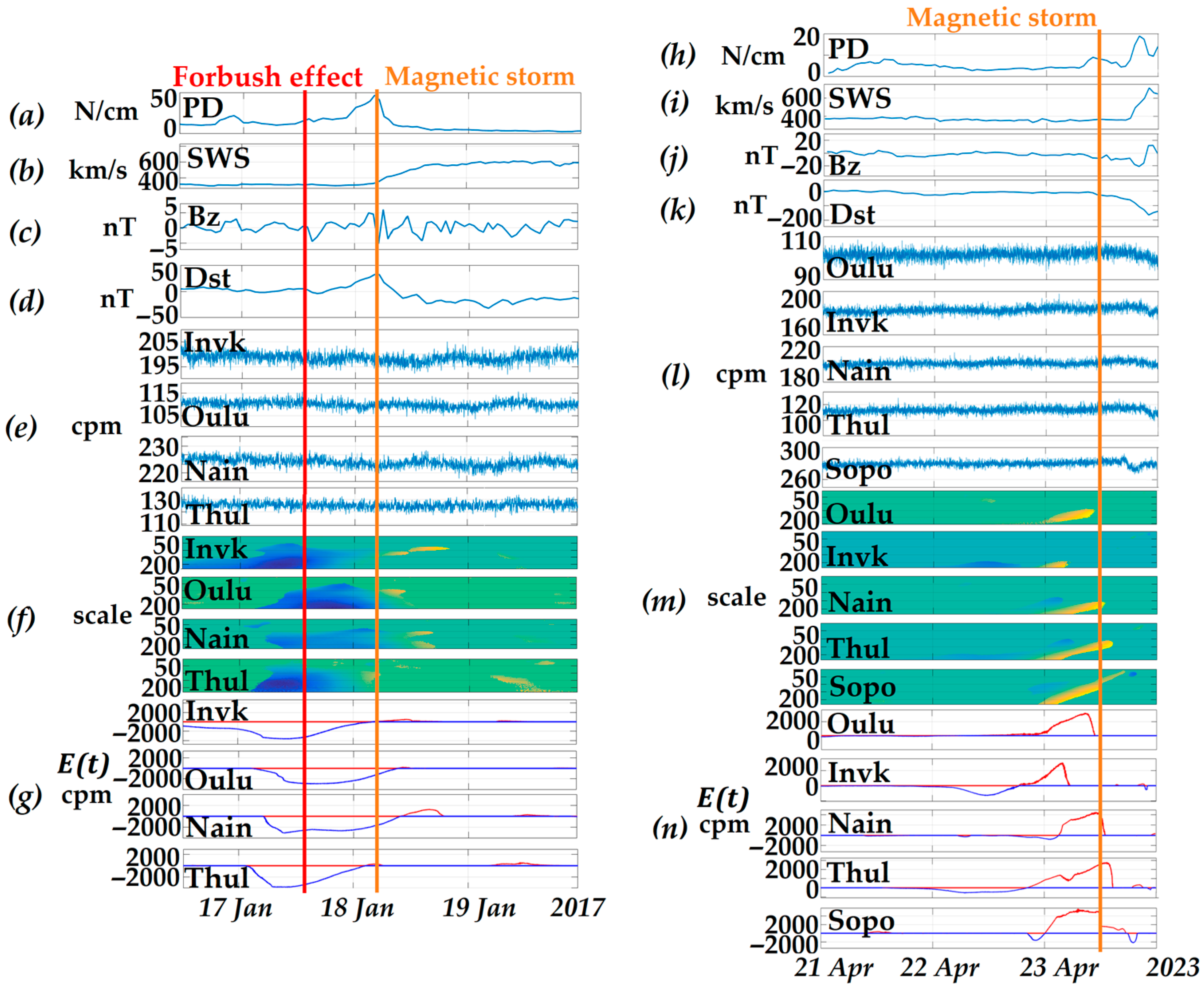
Figure 8 illustrates the results of the suggested method with the NM data from different stations. An example, containing the period of Forbush decrease in cosmic ray variations (Figure 8 on the left) and the period containing an anomalous decrease in cosmic ray intensity (Figure 8 on the right), is shown. The times of the magnetic storm commencements are indicated in Figure 8 by yellow lines. The time of the Forbush decrease according to the data [34] (global survey method was applied) is indicated in Figure 8 by a red line. The results in Figure 8 illustrate that the proposed method made it possible to detect the anomalies in cosmic ray variations timely. We should also note that the Forbush decrease occurrence was determined by the suggested method much earlier (Figure 8 on the left, marked by blue) compared to the global survey method (Figure 8 on the left, marked by a red line). Moreover, the comparison of the results from different stations shows the high sensitivity of the HMTS method and the ability to detect anomalies by the data from each separate station. That indicates high efficiency of the method and the possibility to minimize the number of engaged stations when detecting anomalies in cosmic ray variations. This is an important advantage of the HMTS compared to the global survey method.

5. Conclusions

The paper suggested the hybrid model of a nonstationary time series (HMTS) including the neural network component and the nonlinear adaptive approximating scheme. The HMTS parameters were estimated using the data of neutron monitor ground stations, recording cosmic ray intensities in the near-Earth space. To estimate the HMTS efficiency, model data were also used. Their structure corresponded to neutron monitor data. The estimates showed the high accuracy of the method in the problem of anomaly detection:

• The HMTS regular component adequately describes neutron monitor time series during the periods of anomaly absence. The MSE model values are close to 0 and errors are the Gaussian noise.
• During the anomalous periods, the neural network model errors increase that makes it possible to detect anomalies effectively.
• The detection probability of the anomaly, lasting for 20 counts, is more than 80% for the signal–noise ratio of 1.5 (at the false alarm rate $\alpha =0.05$). When the anomaly lasts for more than 60 counts, the detection probability is close to 90% for the signal–noise ratio equal to 1.3.

Comparison of the HMTS with continuous wavelet transform confirmed the HMTS efficiency in the problems of data analysis and anomaly detection. In the result of the correlated noise effect (including the solar-diurnal cycle of the neutron monitor data), it was impossible to detect an anomaly in the data based on the continuous wavelet transform. Application of the method allowed us to detect the anomaly against the background of correlated noise.

The processing results for the data from different neutron monitor stations showed the high sensitivity of the HMTS. Application of the HMTS made it possible to detect the anomalies based on the data from each separate station compared to the widely applied method of global survey. This shows the possibility to minimize the number of engaged stations when detecting anomalies in cosmic ray variations. The continuous operation of neutron monitor stations is not always provided, thus, this result is important.

The developed HMTS can be recommended for anomaly detection in neutron monitor data, and it is effective even for a small number of operating stations. Moreover, the HMTS can be recommended for the modeling and analysis of nonstationary time series including regular components of nonlinear structures and local features of different form and duration.