A Successive over Relaxation Implicit Iterative Algorithm for Solving Stochastic Linear Systems with Markov Jumps

Abstract

In order to solve continuous stochastic Lyapunov equations, a novel implicit iterative algorithm is presented by means of successive over relaxation (SOR) iteration in this article. Throughout this method, three tuning parameters are added for the improvement of the convergence rate. It is shown that this algorithm is monotonically bounded, and the convergence condition is also given and extended. Applying the latest updated estimates, this algorithm can attain a better convergence performance compared with other existing iterative algorithms when choosing appropriate tuning parameters. Finally, a numerical example is provided to illustrate the feasibility and priority of this approach.

1. Introduction

In the design of control systems, various matrix equations are widely used [1,2,3,4,5,6]. Specifically, some coupled matrix equations are important tools for studying the stability of Markov jump linear systems [7]. It can be seen in [8] that the mean square stability of an Itô system can be characterized by the corresponding Lyapunov-type matrix equation. Markov jump systems are useful tools that have been instrumental in modeling certain real-world systems susceptible to random factors. This concept, which is highlighted by reference [9], has garnered significant interest among researchers within this discipline. By employing Markov jumps, scientists and engineers can gain insight into how various components of these complex systems might behave under conditions of uncertainty or change, providing valuable tools for predicting outcomes and making informed decisions. In [10], the notation of exact detectability is presented for linear systems with state-multiplicative noise. Based on critical stability and exact detectability, some useful properties are derived in [10] for Itô Lyapunov matrix equations. Uniform definitions are given for the notions of observable and detectable properties in the realm of continuous-time stochastic systems reported in [11], where the so-called stochastic Lyapunov matrix equations are reviewed. In [12], some stochastic stability properties are presented for the Markov jump linear system owing to the existence of the solution of coupled Lyapunov matrix equations (CLMEs). In the study referenced in [13], an approach is developed to design a suboptimal controller, denoted as $H_2$/$H_{\infty }$, specifically for continuous-time linear Itô stochastic systems with Markov jumps (MJIS systems). The extended concept of exact detectability in the literature [14] has been incorporated into the linear MJIS systems, making it more convenient to analyze the properties of control systems. Research has suggested that under exact detectability conditions, the mean square stability of a linear MJIS system depends on whether the corresponding Lyapunov matrix equations have positive semi-definite solutions. Two iterative algorithms are established for both continuous-time and discrete-time MJIS systems in [15]. And their convergence are studied using linear positive operators. According to the characteristic of the solution of corresponding Lyapunov equations, a necessary and sufficient condition for the mean square stability of detectable systems of this type is developed in [16]. In fact, the CLMEs, characterized by their intricate coupling dynamics and appearance in MJIS systems, can indeed be considered as a peculiar example of generalized ones.

For the above case, ref. [17] proposes a novel implicit iterative approach specifically tailored to the solution of the CLMEs in discrete-time situations. Ref. [18] proposes a method to tackle the complex challenge of solving coupled equations, through minimizing a quadratic function embedded within the iterative process. In addition, ref. [19] provides a direct method for the coupled matrix equations, which is less effective for large-scale systems. In recent years, various kinds of iterative methods have been put forward by different researchers. Ref. [20] presents a new method of least-square iteration to deal with equations of this kind, in which a hierarchical identification principle is employed. In [21], a full-rank gradient-based algorithm, as well as a reduced-rank one, is constructed. In fact, due to the similarity of coupled and general Lyapunov matrix equations, both can be solved by applying the iterative algorithms. Moreover, all of the above algorithms use the latest estimated value generated by the last iteration process.

In 2016, an implicit iterative algorithm [22] was put forward to solve continuous CLMEs by using some adjustable parameters. The successive over relaxation (SOR) technique is known to be a classic way to increase the convergence rate of Jacobi iterations in [23]. Due to this advantage, it was used to solve the discrete periodic Lyapunov matrix equations [24]. In [25], a novel iterative algorithm is proposed to deal with coupled Lyapunov equations arising in continuous-time Itô stochastic systems with Markov jumps, in which two adjustment parameters are introduced. And it combines both the latest and the former step information to estimate the unknown matrices. Ref. [26] establishes a new iterative method for solving the CLMEs associated with continuous-time Markov jump linear systems by the SOR technique. A relaxation parameter is included, which can be selected appropriately to improve the convergence performance.

Inspired by the aforementioned facts, an SOR implicit iterative algorithm is established in this paper for solving continuous stochastic Lyapunov equations. And three tunable parameters are included to improve the convergence speed of the algorithm. Subsequently, the monotonicity and boundedness of the proposed algorithm are analyzed, and the convergence condition is further investigated. With the up-to-date knowledge of the iteration value, this approach exhibits better convergence than others by choosing the tuning parameters appropriately.

In this paper, we use ${\mathbb{R}}^{m\times n}$ to represent the set of all the $m\times n$-dimensional real matrices. $E(·)$ denotes the mathematical expectation. And $A^T$, $A^{-1}$ represent the transpose and inverse matrices of A, respectively. $\rho \left(A\right)$ is written as the spectral radius of A. The notation $\mathbb{I}[a,b]$ denotes a discrete finite set $\{a,a+1,\cdots ,b\}$, in which both a and b are integers and $a<b$. The vectorization of a matrix $A=[a_1,a_2,\cdots ,a_n]\in {\mathbb{R}}^{n\times n}$ is defined as $vec\left(A\right)={[a_1^T,a_2^T,\cdots ,a_n^T]}^T$. $M\otimes W$ means the Kronecker product of matrices M and W. If P is a positive definite matrix, we record it as $P>0$. Similarly, $(P_1\left(m\right),P_2\left(m\right),\cdots ,P_N\left(m\right))>0$ indicates that in this sequence, $P_i\left(m\right)>0,i\in \mathbb{I}[1,N]$. ${∥·∥}_F$ is used to represent Frobenius norm.

2. Problem Formulation and Preliminaries

There exists a continuous-time Itô stochastic system with Markov jumps:

$$dx\left(t\right)=A_0\left(\theta \left(t\right)\right)x\left(t\right)dt+\sum _{s=1}^r{A}_s\left(\theta \left(t\right)\right)x\left(t\right)d{\omega }_s\left(t\right),$$

(1)

where $x\left(t\right)\in {\mathbb{R}}^n$ is the system state; $A_0\left(\theta \left(t\right)\right)$, $A_s\left(\theta \left(t\right)\right)$ are both the coefficient matrices; ${\omega }_s\left(t\right)\in \mathbb{R},s\in \mathbb{I}[1,r]$ are real random processes, which are defined on a complete probability space $\{\Omega ,\mathcal{F},\mathcal{P}\}$ with $E\left({\omega }_i\left(t\right)\right)=0$ and $E\left({\omega }_i\left(t\right){\omega }_j\left(s\right)\right)={\delta }_{ij},i,j\in \mathbb{I}[1,r]$. $\left\{\theta \right(t),t⩾0\}$ is a continuous-time discrete-state Markov process. The transition rate matrix is $\Pi ={\left[{\pi }_{ij}\right]}_{N\times N}$, while ${\pi }_{ij}⩾0$ for $j\ne i$, and ${\sum }_{j=1}^N{\pi }_{ij}=0$, $i\in \mathbb{I}[1,N]$. The initial values are set to be $x\left(0\right)=x_0$ and $\theta \left(0\right)={\theta }_0$. Next, the definition of asymptotically mean square stability (AMSS) is introduced for system (1).

Definition 1 ([15]).

System (1) has AMSS if for any $x_0\in {\mathbb{R}}^n$ and ${\theta }_0\in \mathbb{I}[1,N]$, there exists

$$\underset{t\to \infty }{lim}E\left({∥x(t,x_0,{\theta }_0)∥}^2\right|x_0,{\theta }_0)=0.$$

The corresponding continuous stochastic Lyapunov equation of system (1) can be written as follows:

$$\begin{array}{c}\hfill A_{0i}^T{P}_i+P_i{A}_{0i}+\sum _{s=1}^r{A}_{si}^T{P}_i{A}_{si}+\sum _{j=1}^N{\pi }_{ij}{P}_j=-Q_i,i\in \mathbb{I}[1,N].\end{array}$$

(2)

In this equation, $P_i,i\in \mathbb{I}[1,N]$ are unknown solutions of Lyapunov Equation (2) and $Q_i>0$, $i\in \mathbb{I}[1,N]$, are known matrices. This equation is usually used to analyze the stability of system (1). Regarding the asymptotically mean square stability of (1), the following result is obtained.

Lemma 1 ([15]).

System (1) has AMSS if and only if there is a unique solution $(P_1,P_2,\cdots$$,P_N)>0$ of the corresponding Lyapunov Equation (2), for any given $Q_i>0$.

Thus, the stability of the system (1) is equivalent to finding a unique solution of Equation (2). While Lyapunov Equation (2) can be changed into the following format:

$$A_i^T{P}_i+P_i{A}_i=-\sum _{s=1}^r{A}_{si}^T{P}_i{A}_{si}-\sum _{j=1,j\ne i}^N{\pi }_{ij}{P}_j-{\beta }_i{P}_i-Q_i,$$

(3)

with

$$A_i=A_{0i}+0.5{\pi }_{ii}{I}_n-0.5{\beta }_i{I}_n,{\beta }_i⩾0,i\in \mathbb{I}[1,N].$$

(4)

Through Lemma 1 and the associated theories of stability, we can obtain the following conclusions:

Lemma 2 ([25]).

Any matrix $A_i$, $i\in \mathbb{I}[1,N]$ is Hurwitz-stable if system (1) has AMSS.

An iterative algorithm in the implicit form is proposed in [25] to deal with the coupled Lyapunov Equation (2). It is summarized as follows:

Theorem 1 ([25]).

Assume the Markov jump system (1) has AMSS. If the following algorithm (5) satisfies $Q_i>0$, ${\beta }_i⩾0$, and the tuning parameters ${\alpha }_j\in [0,1]$, then the sequence $(P_1\left(m\right),P_2\left(m\right),\cdots$, $P_N\left(m\right))$ generated by the algorithm (5) with zero initial conditions $P_i\left(0\right)=0$, $i\in \mathbb{I}[1,N]$ converges to the unique positive definite solution of the continuous coupled Lyapunov matrix Equation (2). The following is the designed iteration form:

$$\begin{array}{cc}\hfill A_i^T{P}_i(m+1)+P_i(m+1)A_i=& -\sum _{s=1}^r{A}_{si}^T{P}_i\left(m\right)A_{si}-\sum _{j=1}^{i-1}{\pi }_{ij}[{\alpha }_j{P}_j(m+1)\hfill \\ \hfill & +(1-{\alpha }_j)P_j\left(m\right)]-\sum _{j=i+1}^N{\pi }_{ij}{P}_j\left(m\right)\hfill \\ & -{\beta }_i{P}_i\left(m\right)-Q_i,i\in \mathbb{I}[1,N].\hfill \end{array}$$

(5)

3. Main Result

Enlightened by the idea of SOR technique, in what follows, we plan to find a new algorithm to obtain the solution of Equation (2). Since we have

$$A_i^T{P}_i+P_i{A}_i=(1-\gamma )(A_i^T{P}_i+P_i{A}_i)+\gamma (A_i^T{P}_i+P_i{A}_i),i\in \mathbb{I}[1,N],$$

(6)

and $\gamma$ is a tunable parameter. From the preceding section, we rewrite Equation (2) as (3) by substituting the first term on the right-hand side of (6) with the right-hand item of (3); we obtain the following relation:

$$\begin{array}{cc}\hfill A_i^T{P}_i+P_i{A}_i=& (1-\gamma )(-\sum _{s=1}^r{A}_{si}^T{P}_i{A}_{si}-\sum _{j=1}^{i-1}{\pi }_{ij}[{\alpha }_j{P}_j+(1-{\alpha }_j)P_j]\hfill \\ & -\sum _{j=i+1}^N{\pi }_{ij}{P}_j-{\beta }_i{P}_i-Q_i)+\gamma (A_i^T{P}_i+P_i{A}_i),i\in \mathbb{I}[1,N].\hfill \end{array}$$

(7)

Utilizing the latest updated estimation, we bring up an implicit iterative algorithm below to solve Equation (2):

$$\begin{array}{cc}\hfill A_i^T{P}_i(m+1)+P_i& (m+1)A_i\hfill \\ \hfill =& (1-\gamma )(-\sum _{s=1}^r{A}_{si}^T{P}_i\left(m\right)A_{si}-\sum _{j=1}^{i-1}{\pi }_{ij}[{\alpha }_j{P}_j(m+1)\hfill \\ & +(1-{\alpha }_j)P_j\left(m\right)]-\sum _{j=i+1}^N{\pi }_{ij}{P}_j\left(m\right)-{\beta }_i{P}_i\left(m\right)-Q_i)\hfill \\ & +\gamma (A_i^T{P}_i\left(m\right)+P_i\left(m\right)A_i),i\in \mathbb{I}[1,N].\hfill \end{array}$$

(8)

Remark 1.

If the parameter $\gamma =0$, then the proposed algorithm (8) is reduced to algorithm (5).

Remark 2.

For every iteration step of algorithm (8), N standard continuous Lyapunov matrix equations need to be solved. The algorithm proposed in this paper is an implicit form.

Remark 3.

It can be seen that the algorithm (8) proposed in this article is very similar to the SOR iteration method in ordinary linear equations. Therefore, in the following text, algorithm (8) is abbreviated as the SOR implicit iterative algorithm.

First, the following lemma illustrates that the sequence generated by (8) is bounded.

Lemma 3.

Assume system (1) has AMSS, and $Q_i>0$, $i\in \mathbb{I}[1,N]$. If ${\beta }_i⩾0$, and the tuning parameters ${\alpha }_j\in [0,1]$, then on the condition of zero initial values, there is an upper bound of the sequence $(P_1\left(m\right),P_2\left(m\right),\dots$$,P_N\left(m\right))$ generated by algorithm (8) when $0\le \gamma <1$. In other words, for any integer $m⩾0$, we have

$$P_i\left(m\right)<P_i,i\in \mathbb{I}[1,N].$$

(9)

Proof. 

According to Lemmas 1 and 2, since the matrices $A_i$, $i\in \mathbb{I}[1,N]$ are Hurwitz-stable and Equation (2) has a unique solution $(P_1,P_2,\cdots$$,P_N)$, we can subtract (8) from (7) to obtain

$$A_i^T[P_i-P_i(m+1)-\gamma (P_i-P_i\left(m\right))]+[P_i-P_i(m+1)-\gamma (P_i-P_i\left(m\right))]A_i=V_i\left(m\right),$$

(10)

and

$$\begin{array}{cc}\hfill V_i\left(m\right)=& (1-\gamma )(-\sum _{s=1}^r{A}_{si}^T(P_i-P_i\left(m\right))A_{si}-\sum _{j=1}^{i-1}{\pi }_{ij}[{\alpha }_j(P_j-P_j(m+1))\hfill \\ & +(1-{\alpha }_j)(P_j-P_j\left(m\right))]-\sum _{j=i+1}^N{\pi }_{ij}(P_j-P_j\left(m\right))\hfill \\ & -{\beta }_i(P_i-P_i\left(m\right))).\hfill \end{array}$$

(11)

In the following text, the proof of this theorem is mainly based on mathematical induction. Because of the zero initial value condition of the algorithm mentioned before, apparently, (9) holds for $m=0$. Now, we suppose when $m=k$ and $k⩾0$, (9) holds. This means

$$P_i\left(k\right)<P_i,i\in \mathbb{I}[1,N].$$

(12)

Let $m=k$, $i=1$ in relation (11); we can obtain

$$\begin{array}{cc}\hfill V_1\left(k\right)=& (1-\gamma )(-\sum _{s=1}^r{A}_{s1}^T(P_1-P_1\left(k\right))A_{s1}-\sum _{j=2}^N{\pi }_{1j}(P_j-P_j\left(k\right))\hfill \\ & -{\beta }_1(P_1-P_1\left(k\right))).\hfill \end{array}$$

(13)

Due to the assumptions set by mathematical induction above and $0\le \gamma <1$, we can obtain $V_1\left(k\right)<0$. Therefore, from (10), we know that

$$A_1^T[P_1-P_1(k+1)-\gamma (P_1-P_1\left(k\right))]+[P_1-P_1(k+1)-\gamma (P_1-P_1\left(k\right))]A_1<0.$$

(14)

$A_1$ is Hurwitz-stable, so we can obtain the following inequality from Theorem 3.1 in [27]:

$$P_1-P_1(k+1)-\gamma (P_1-P_1\left(k\right))>0.$$

That is,

$$P_1-P_1(k+1)>\gamma (P_1-P_1\left(k\right)).$$

Since $P_1>P_1\left(k\right)$ from assumption (12), we have

$$P_1>P_1(k+1).$$

(15)

Using mathematical induction again, we now assume that

$$P_j>P_j(k+1),j\in \mathbb{I}[1,l-1],l⩾2.$$

(16)

Let $m=k$, $i=l$ in Equations (10) and (11); we can obtain

$$A_l^T[P_l-P_l(k+1)-\gamma (P_l-P_l\left(k\right))]+[P_l-P_l(k+1)-\gamma (P_l-P_l\left(k\right))]A_l=V_l\left(k\right),$$

and

$$\begin{array}{cc}\hfill V_l\left(k\right)=(1& - \gamma \left)\right(-\sum _{s=1}^r{A}_{sl}^T(P_l-P_l\left(k\right))A_{sl}-\sum _{j=1}^{l-1}{\pi }_{lj}[{\alpha }_j(P_j-P_j(k+1))\hfill \\ & +(1-{\alpha }_j)(P_j-P_j\left(k\right))]-\sum _{j=l+1}^N{\pi }_{lj}(P_j-P_j\left(k\right))-{\beta }_l(P_l-P_l\left(k\right))).\hfill \end{array}$$

For $0\le \gamma <1$; from assumptions (12) and (16), we can obtain $V_l\left(k\right)<0$. That is,

$$A_l^T[P_l-P_l(k+1)-\gamma (P_l-P_l\left(k\right))]+[P_l-P_l(k+1)-\gamma (P_l-P_l\left(k\right))]A_l<0.$$

Due to the Hurwitz stability of $A_l$, the following inequality holds:

$$P_l-P_l(k+1)-\gamma (P_l-P_l\left(k\right))>0.$$

It means that

$$P_l-P_l(k+1)>\gamma (P_l-P_l\left(k\right)).$$

According to assumption (12), we have the conclusion $P_l>P_l(k+1)$. Combine it with relation (16), by knowledge of mathematical induction, we know that

$$P_i>P_i(k+1),i\in \mathbb{I}[1,N].$$

(17)

Eventually, with (17) and assumption (12), it could be summarized that for any integer $m⩾0$, (9) holds. Thus, we complete this proof. □

Second, it is found that the sequence generated by (8) is monotonically increasing.

Lemma 4.

Assume that system (1) has AMSS, and $Q_i>0$, $i\in \mathbb{I}[1,N]$. If ${\beta }_i⩾0$, $0\le \gamma <1$, and the tuning parameters ${\alpha }_j\in [0,1]$, then on the condition of zero initial values, the sequence $(P_1\left(m\right),P_2\left(m\right),\dots$$,P_N\left(m\right))$ produced by algorithm (8) is strictly monotonically incremental. In other words, for any integer $m⩾0$, we have

$$P_i\left(m\right)<P_i(m+1),i\in \mathbb{I}[1,N].$$

(18)

Proof. 

The matrices $A_i$, $i\in \mathbb{I}[1,N]$ are Hurwitz-stable and Equation (2) has the only solution $(P_1,P_2,\dots$$,P_N)$ according to Lemmas 1 and 2. Let $m=k$ and $m=k+1$ in (8); subtract the former from the latter to obtain

$$\begin{array}{cc}\hfill A_i^T[P_i& (k+2)-P_i(k+1)-\gamma (P_i(k+1)-P_i\left(k\right))]\hfill \\ \hfill +& [P_i(k+2)-P_i(k+1)-\gamma (P_i(k+1)-P_i\left(k\right))]A_i=M_i\left(k\right),\hfill \end{array}$$

(19)

where

$$\begin{array}{cc}\hfill M_i\left(k\right)=(1& - \gamma \left)\right(-\sum _{s=1}^r{A}_{si}^T(P_i(k+1)-P_i\left(k\right))A_{si}\hfill \\ & -\sum _{j=1}^{i-1}{\pi }_{ij}[{\alpha }_j(P_j(k+2)-P_j(k+1))\hfill \\ & +(1-{\alpha }_j)(P_j(k+1)-P_j\left(k\right))]\hfill \\ & -\sum _{j=i+1}^N{\pi }_{ij}(P_j(k+1)-P_j\left(k\right))\hfill \\ & -{\beta }_i(P_i(k+1)-P_i\left(k\right))),i\in \mathbb{I}[1,N].\hfill \end{array}$$

(20)

Subsequently, mathematical induction is utilized to help prove the above lemma. Since $P_i\left(0\right)=0,i\in \mathbb{I}[1,N]$, it is easily known that (18) holds for $m=0$. Now, we suppose when $m=k,k⩾0,$ (18) holds, which means

$$P_i\left(k\right)<P_i(k+1),i\in \mathbb{I}[1,N].$$

(21)

Let $i=1$ in (20); we can obtain

$$\begin{array}{cc}\hfill M_1\left(k\right)=(1& - \gamma \left)\right(-\sum _{s=1}^r{A}_{s1}^T(P_1(k+1)-P_1\left(k\right))A_{s1}\hfill \\ & -\sum _{j=2}^N{\pi }_{1j}(P_j(k+1)-P_j\left(k\right))-{\beta }_1(P_1(k+1)-P_1\left(k\right))).\hfill \end{array}$$

(22)

For $0\le \gamma <1$, according to assumption (21), it can be easily found that $M_1\left(k\right)<0$. Therefore, from (19), we can obtain the following inequality:

$$\begin{array}{cc}\hfill A_1^T[& P_1(k+2)-P_1(k+1)-\gamma (P_1(k+1)-P_1\left(k\right))]\hfill \\ & +[P_1(k+2)-P_1(k+1)-\gamma (P_1(k+1)-P_1\left(k\right))]A_1<0.\hfill \end{array}$$

(23)

For the Hurwitz stability of $A_1$, we have the following inequality from Theorem 3.1 in [27]:

$$P_1(k+2)-P_1(k+1)-\gamma (P_1(k+1)-P_1\left(k\right))>0.$$

Equivalently,

$$P_1(k+2)-P_1(k+1)>\gamma (P_1(k+1)-P_1\left(k\right)).$$

From assumption (21) that $P_1(k+1)>P_1\left(k\right)$, we have

$$P_1(k+2)>P_1(k+1).$$

(24)

Using mathematical induction repeatedly, we now assume that

$$P_j(k+2)>P_j(k+1),j\in \mathbb{I}[1,l-1],l⩾2.$$

(25)

For relation (20), let $i=l$; we can obtain

$$\begin{array}{cc}\hfill M_l\left(k\right)=(1& - \gamma \left)\right(-\sum _{s=1}^r{A}_{sl}^T(P_l(k+1)-P_l\left(k\right))A_{sl}\hfill \\ & -\sum _{j=1}^{l-1}{\pi }_{lj}[{\alpha }_j(P_j(k+2)-P_j(k+1))\hfill \\ & +(1-{\alpha }_j)(P_j(k+1)-P_j\left(k\right))]\hfill \\ & -\sum _{j=l+1}^N{\pi }_{lj}(P_j(k+1)-P_j\left(k\right))\hfill \\ & -{\beta }_l(P_l(k+1)-P_l\left(k\right))).\hfill \end{array}$$

Since $0\le \gamma <1$, if induction assumptions (21) and (25) hold, we can obtain $M_l\left(k\right)<0$. For relation (19) with $i=l$, we have that

$$\begin{array}{cc}\hfill A_l^T\left[P_l\right(k& + 2) - P_l(k+1)-\gamma (P_l(k+1)-P_l\left(k\right))]\hfill \\ \hfill +& [P_l(k+2)-P_l(k+1)-\gamma (P_l(k+1)-P_l\left(k\right))]A_l<0.\hfill \end{array}$$

(26)

$A_l$ is Hurwitz-stable; hence,

$$P_l(k+2)-P_l(k+1)-\gamma (P_l(k+1)-P_l\left(k\right))>0.$$

This is equivalent to

$$P_l(k+2)-P_l(k+1)>\gamma (P_l(k+1)-P_l\left(k\right)).$$

In terms of assumption (21), we have $P_l(k+2)>P_l(k+1)$. Based on this and relation (25), the following is evident from mathematical induction:

$$P_i(k+2)>P_i(k+1),i\in \mathbb{I}[1,N].$$

(27)

Consequently, with (27) and assumption (21), it is proven that for any integer $m⩾0$, (18) holds. Thus, the proof is finished. □

Combining Lemmas 3 and 4, the following convergence property of algorithm (8) can be deduced.

Theorem 2.

Assume system (1) has AMSS, and $Q_i>0$, $i\in \mathbb{I}[1,N]$. If ${\beta }_i⩾0$, $0\le \gamma <1$, and the tuning parameters ${\alpha }_j\in [0,1]$, then on the condition of zero initial values $P_i\left(0\right)=0$, $i\in \mathbb{I}[1,N]$, the sequence $(P_1\left(m\right),P_2\left(m\right),\dots$$,P_N\left(m\right))$ produced by algorithm (8) monotonically converges to the unique solution $(P_1,P_2,...,P_N)$ of Equation (2).

Proof. 

From Lemmas 3 and 4 and the conditions of Theorem 2, the sequence $(P_1\left(m\right),P_2\left(m\right),$$\cdots ,P_N\left(m\right))$ produced by the SOR implicit algorithm (8) increases monotonically and has an upper bound, which is the solution of (2). It means that

$$0=P_i\left(0\right)<P_i\left(1\right)<P_i\left(2\right)<\cdots <P_i\left(N\right)<P_i,i\in \mathbb{I}[1,N].$$

Thus, the sequence $(P_1\left(m\right),P_2\left(m\right),\cdots ,P_N\left(m\right))$ is convergent. Take the limit on $P_i\left(k\right)$, and denote

$$\underset{k\to \infty }{lim}{P}_i\left(k\right)=P_{i\infty },i\in \mathbb{I}[1,N].$$

By simultaneously taking limits on both sides of algorithm (8), we can easily obtain

$$\begin{array}{cc}\hfill A_i^T{P}_{i\infty }+P_{i\infty }{A}_i=(1& - \gamma \left)\right(-\sum _{s=1}^r{A}_{si}^T{P}_{i\infty }{A}_{si}-\sum _{j=1}^{i-1}{\pi }_{ij}[{\alpha }_j{P}_{j\infty }+(1-{\alpha }_j)P_{j\infty }]\hfill \\ & -\sum _{j=i+1}^N{\pi }_{ij}{P}_{j\infty }-{\beta }_i{P}_{i\infty }-Q_i)+\gamma (A_i^T{P}_{i\infty }+P_{i\infty }{A}_i).\hfill \end{array}$$

This is equivalent to

$$\begin{array}{cc}\hfill (A_{0i}+0.5& {\pi }_{ii}{I}_n-0.5{\beta }_i{I}_n{)}^T{P}_{i\infty }+P_{i\infty }(A_{0i}+0.5{\pi }_{ii}{I}_n-0.5{\beta }_i{I}_n)\hfill \\ \hfill =(& 1-\gamma \left)\right(-\sum _{s=1}^r{A}_{si}^T{P}_{i\infty }{A}_{si}-\sum _{j=1}^{i-1}{\pi }_{ij}[{\alpha }_j{P}_{j\infty }+(1-{\alpha }_j)P_{j\infty }]\hfill \\ & -\sum _{j=i+1}^N{\pi }_{ij}{P}_{j\infty }-{\beta }_i{P}_{i\infty }-Q_i)+\gamma [{(A_{0i}+0.5{\pi }_{ii}{I}_n-0.5{\beta }_i{I}_n)}^T{P}_{i\infty }\hfill \\ & +P_{i\infty }(A_{0i}+0.5{\pi }_{ii}{I}_n-0.5{\beta }_i{I}_n)],\hfill \end{array}$$

so

$$\begin{array}{cc}\hfill (1-\gamma )& [{(A_{0i}+0.5{\pi }_{ii}{I}_n-0.5{\beta }_i{I}_n)}^T{P}_{i\infty }+P_{i\infty }(A_{0i}+0.5{\pi }_{ii}{I}_n-0.5{\beta }_i{I}_n)]\hfill \\ \hfill =& (1-\gamma )(-\sum _{s=1}^r{A}_{si}^T{P}_{i\infty }{A}_{si}-\sum _{j=1}^{i-1}{\pi }_{ij}[{\alpha }_j{P}_{j\infty }+(1-{\alpha }_j)P_{j\infty }]\hfill \\ & -\sum _{j=i+1}^N{\pi }_{ij}{P}_{j\infty }-{\beta }_i{P}_{i\infty }-Q_i)\hfill \\ \hfill =& (1-\gamma )\left(-\sum _{s=1}^r{A}_{si}^T{P}_{i\infty }{A}_{si}-\sum _{j=1}^N{\pi }_{ij}{P}_{j\infty }+{\pi }_{ii}{P}_{i\infty }-{\beta }_i{P}_{i\infty }-Q_i\right).\hfill \end{array}$$

Dividing both sides by $1-\gamma$ simultaneously, we obtain

$$\begin{array}{cc}\hfill (A_{0i}+0.5& {\pi }_{ii}{I}_n-0.5{\beta }_i{I}_n{)}^T{P}_{i\infty }+P_{i\infty }(A_{0i}+0.5{\pi }_{ii}{I}_n-0.5{\beta }_i{I}_n)\hfill \\ \hfill =& -\sum _{s=1}^r{A}_{si}^T{P}_{i\infty }{A}_{si}-\sum _{j=1}^N{\pi }_{ij}{P}_{j\infty }+{\pi }_{ii}{P}_{i\infty }-{\beta }_i{P}_{i\infty }-Q_i,\hfill \end{array}$$

which can be equivalently written as follows:

$$A_{0i}^T{P}_{i\infty }+P_{i\infty }{A}_{0i}+\sum _{s=1}^r{A}_{si}^T{P}_{i\infty }{A}_{si}+\sum _{j=1}^N{\pi }_{ij}{P}_{j\infty }=-Q_i.$$

(28)

Compared with matrix Equation (2), we find that the sequence $(P_{1\infty },P_{2\infty },\cdots ,P_{N\infty })$ is exactly the same solution of the coupled Lyapunov matrix Equation (2). □

It has been demonstrated that algorithm (8) can operate under a zero initial condition. However, this condition is too harsh. Consequently, a sufficient condition is provided for the convergence of algorithm (8) under an arbitrary initial value.

Theorem 3.

Assume that system (1) has AMSS, and $Q_i>0$, $i\in \mathbb{I}[1,N]$. Matrices M and W are expressed from Equation (29) as follows:

$$M=-diag\left(I_n\otimes A_1^T+A_1^T\otimes I_n,I_n\otimes A_2^T+A_2^T\otimes I_n,\cdots ,I_n\otimes A_N^T+A_N^T\otimes I_n\right)+(1-\gamma )\underline{M},$$

where

$$\underline{M}=-\left[\begin{array}{ccccc}0& 0& \cdots & 0& 0\\ {\alpha }_1{\pi }_{21}{I}_{n^2}& 0& \cdots & 0& 0\\ \cdots & \cdots & \ddots & \cdots & \cdots \\ {\alpha }_1{\pi }_{N-1,1}{I}_{n^2}& a_2{\pi }_{N-1,2}{I}_{n^2}& \cdots & 0& 0\\ a_1{\pi }_{N1}{I}_{n^2}& a_2{\pi }_{N2}{I}_{n^2}& \cdots & {\alpha }_{N-1}{\pi }_{N,N-1}{I}_{n^2}& 0\end{array}\right].$$

And

$$\begin{array}{cc}\hfill W=& -\gamma diag\left(I_n\otimes A_1^T+A_1^T\otimes I_n,I_n\otimes A_2^T+A_2^T\otimes I_n,\cdots ,I_n\otimes A_N^T+A_N^T\otimes I_n\right)\hfill \\ & +(1-\gamma )diag(\sum _{s=1}^r{A}_{s_1}^{\mathrm{T}}\otimes A_{s_1}^{\mathrm{T}}+{\beta }_1{I}_{n^2},\sum _{s=1}^r{A}_{s2}^{\mathrm{T}}\otimes A_{s2}^{\mathrm{T}}+{\beta }_2{I}_{n^2},\cdots ,\sum _{s=1}^r{A}_{sN}^{\mathrm{T}}\otimes A_{sN}^{\mathrm{T}}+{\beta }_N{I}_{n^2})\hfill \\ & +(1-\gamma )\underline{W},\hfill \end{array}$$

where

$$\underline{W}=\left[\begin{array}{ccccc}0& {\pi }_{12}{I}_{n^2}& \cdots & {\pi }_{1,N-1}{I}_{n^2}& {\pi }_{1N}{I}_{n^2}\\ (1-{\alpha }_1){\pi }_{21}{I}_{n^2}& 0& \cdots & {\pi }_{2,N-1}{I}_{n^2}& {\pi }_{2N}{I}_{n^2}\\ ...& ...& \ddots & ...& ...\\ (1-{\alpha }_1){\pi }_{N-1,1}{I}_{n^2}& (1-{\alpha }_2){\pi }_{N-1,2}{I}_{n^2}& ...& 0& {\pi }_{N-1,N}{I}_{n^2}\\ (1-{\alpha }_1){\pi }_{N1}{I}_{n^2}& (1-{\alpha }_2){\pi }_{N2}{I}_{n^2}& ...& (1-{\alpha }_{N-1}){\pi }_{N,N-1}{I}_{n^2}& 0\end{array}\right].$$

If the tuning parameters ${\alpha }_j$ and ${\beta }_i$, and the relaxation parameter γ, satisfy $\rho \left(M^{-1}W\right)<1$, then the sequence $(P_1\left(m\right),P_2\left(m\right),\cdots ,P_N\left(m\right))$ produced by the SOR implicit algorithm (8), and with any initial condition $(P_1\left(0\right),P_2\left(0\right),\cdots ,P_N\left(0\right))$, $i\in \mathbb{I}[1,N]$ will converge to the solution of Equation (2).

Proof. 

We define the vectors $\xi$ and q as

$$\begin{array}{cc}\hfill & \xi ={[{\left[vec\left(P_1\right)\right]}^T,{\left[vec\left(P_2\right)\right]}^T,\dots ,{\left[vec\left(P_N\right)\right]}^T]}^T,\hfill \\ \hfill & \xi \left(m\right)={[{\left[vec\left(P_1\left(m\right)\right)\right]}^T,{\left[vec\left(P_2\left(m\right)\right)\right]}^T,\dots ,{\left[vec\left(P_N\left(m\right)\right)\right]}^T]}^T,\hfill \\ \hfill & q={[{\left[(1-\gamma )vec\left(Q_1\right)\right]}^T,{\left[(1-\gamma )vec\left(Q_2\right)\right]}^T,\dots ,{\left[(1-\gamma )vec\left(Q_N\right)\right]}^T]}^T.\hfill \end{array}$$

Next, algorithm (8) can be rewritten in the form of Kronecker product:

$$\begin{array}{cc}\hfill -(I_n\otimes & A_i^T+A_i^T\otimes I_n)vec\left(P_i(m+1)\right)-(1-\gamma )\sum _{j=1}^{i-1}{\alpha }_j{\pi }_{ij}vec\left(P_j(m+1)\right)\hfill \\ \hfill =(& 1-\gamma )(\sum _{s=1}^r{A}_{si}^T\otimes A_{si}^T+{\beta }_i{I}_{n^2})vec\left(P_i\left(m\right)\right)\hfill \\ & -\gamma (I_n\otimes A_i^T+A_i^T\otimes I_n)vec\left(P_i\left(m\right)\right)\hfill \\ \hfill & +(1-\gamma )\sum _{j=1}^{i-1}{\pi }_{ij}(1-{\alpha }_j)vec\left(P_j\left(m\right)\right)\hfill \\ & +(1-\gamma )\sum _{j=i+1}^N{\pi }_{ij}vec\left(P_j\left(m\right)\right)\hfill \\ & +(1-\gamma )vec\left(Q_i\right).\hfill \end{array}$$

(29)

The definitions of matrices M and W are based on the above equation. Combining the vector $\xi$, q, and matrices M and W defined earlier, we can further obtain

$$M\xi (m+1)=W\xi \left(m\right)+q.$$

By multiplying the inverse matrix of M from the left, we have

$$\xi (m+1)=M^{-1}W\xi \left(m\right)+M^{-1}q.$$

(30)

According to the relationship between the previous and subsequent vectors $\xi$, we can deduce repeatedly and obtain

$$\xi (m+1)={\left(M^{-1}W\right)}^{m+1}\xi \left(0\right)+\sum _{j=0}^m{\left(M^{-1}W\right)}^j{M}^{-1}q.$$

If $\rho \left(M^{-1}W\right)<1$, then when m approaches infinity, ${\left(M^{-1}W\right)}^k$ approaches a zero matrix; hence,

$$\underset{m\to \infty }{lim}\xi (m+1)=\underset{m\to \infty }{lim}\sum _{j=0}^m{\left(M^{-1}W\right)}^j{M}^{-1}q={(M-W)}^{-1}q.$$

(31)

Since the matrix Equation (2) could be rewritten as $\xi ={(M-W)}^{-1}q$, the sequence $\left\{\xi \right(m\left)\right\}$ generated by the SOR algorithm (8) converges to the unique solution of Equation (2). □

4. Illustrative Example

Consider Equation (2), in which $N=2$, $r=1$. $Q_1$, $Q_2$ are both fourth-order identity matrices. The system matrices and probability transition rate matrix $\Pi$ are defined as follows:

$$A_{01}=\left[\begin{array}{cccc}-1.0000& -1.0000& -2.0000& 1.0000\\ -0.6667& -3.5000& 1.0000& 1.1670\\ 1.0000& 0.5000& -3.0000& 0.5000\\ -2.0000& -2.5000& 1.0000& -2.5000\end{array}\right],$$

$$A_{02}=\left[\begin{array}{cccc}-1.3333& 1.0000& -2.0000& 0.3333\\ 0.0000& -3.5000& 1.0000& 1.5000\\ 1.0000& 1.5000& -4.0000& -0.5000\\ -1.3333& -3.5000& 1.0000& -1.1667\end{array}\right],$$

$$A_{11}=\left[\begin{array}{cccc}0.9003& 0.7826& 0.6428& 0.8436\\ -0.5377& 0.5242& -0.1106& 0.4764\\ 0.2137& -0.0871& 0.2309& -0.6475\\ -0.0280& -0.9630& 0.5839& -0.1886\end{array}\right],$$

$$A_{12}=\left[\begin{array}{cccc}0.8709& -0.8842& -0.7222& -0.4556\\ 0.8338& -0.2943& -0.5945& -0.6024\\ -0.1796& 0.6263& -0.6026& -0.9695\\ 0.7873& -0.9803& 0.2076& 0.4936\end{array}\right],$$

$$\Pi =\left[\begin{array}{cc}-0.6& 0.6\\ 1& -1\end{array}\right].$$

This example is used in [25]. The iterative error at step k is defined as

$$ϵ\left(k\right)=\sqrt{\sum _{i=1}^N{∥A_{0i}^T{P}_i\left(k\right)+P_i\left(k\right)A_{0i}+\sum _{s=1}^r{A}_{si}^T{P}_i\left(k\right)A_{si}+\sum _{j=1}^N{\pi }_{ij}{P}_j\left(k\right)+Q_i∥}_F^2}.$$

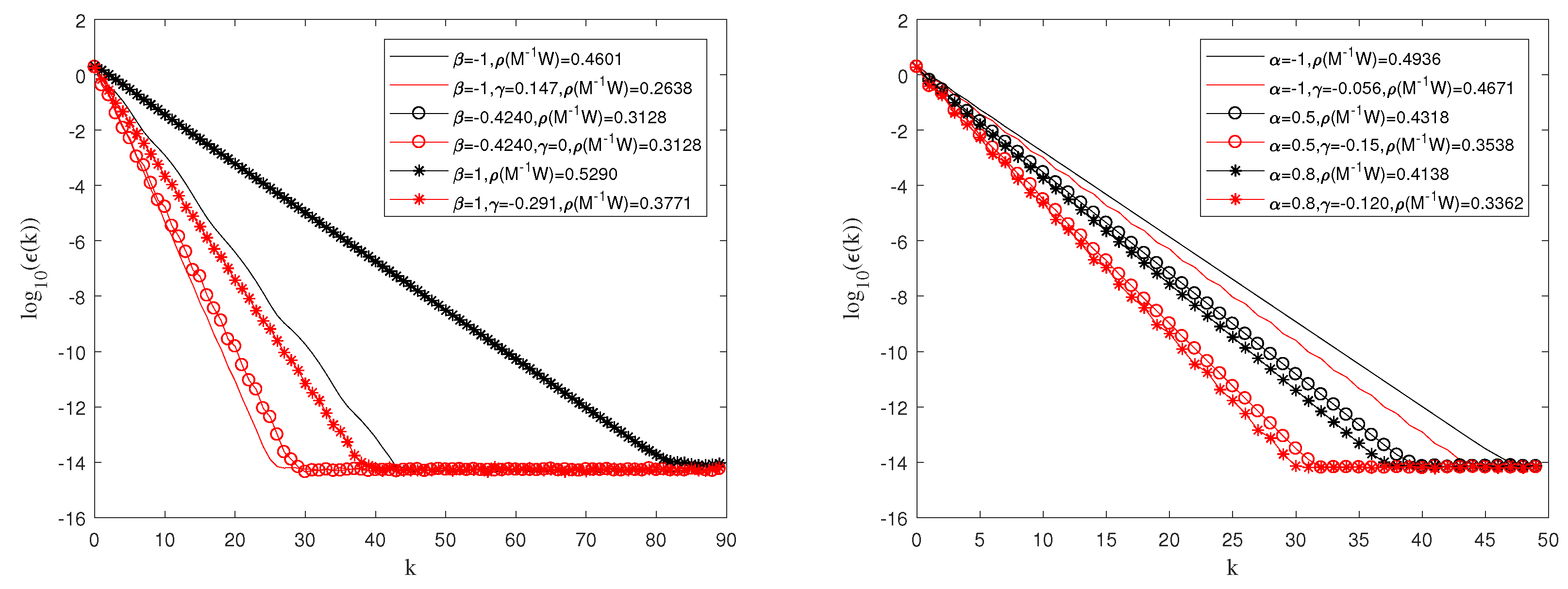
First, we investigated the convergence of algorithm (8) when $\alpha ={\alpha }_1=1$ and $\beta ={\beta }_1={\beta }_2$. The value of $\beta$ was chosen to be the same as that in [25]. In order to make the Figure looks concise, in Figure 1, we only selected three sets of different tuning parameter values from [25] and compared the convergence performance after selecting a proper parameter $\gamma$ with the Matlab function. We found that by adjusting the value of parameter $\gamma$, a smaller spectral radius $\rho \left(M^{-1}W\right)$ and fewer iteration steps k could be obtained. The convergence curves are shown in Figure 1. It should be mentioned that when $\gamma$ takes the value of 0, algorithm (8) degenerates to algorithm (5), which is proposed in [25], so the two algorithms show the same convergence curves. The red convergence curve represents the convergence situation of algorithm (8), while the black curve represents that of algorithm (5). So, it is evident that when the values of $\alpha$ and $\beta$ remained constant, selecting the appropriate parameter $\gamma$ achieved better convergence results. In [25], the minimum spectral radius $\rho \left(M^{-1}W\right)=0.3128$ was gained when $\alpha =1$ and $\beta =-0.4240$. By using the Matlab function, we found that under this condition, it converged fast only when $\gamma$ took the value of 0. But when $\alpha =1$ and $\beta =-1$, we obtained a smaller $\rho \left(M^{-1}W\right)=0.2638$ by choosing $\gamma =0.147$. It is obvious that when the values of $\alpha$ and $\beta$ were chosen to be the same as the algorithm (5) proposed in [25], we achieved a faster convergence rate by selecting different values of parameter $\gamma$ with the help of Matlab (version R2017a).

Figure 1 shows the algorithm’s convergence after selecting appropriate relaxation parameters. The left figure displays the case when $\alpha =1$, and the right figure displays the case when $\beta =0$. The value of $\alpha$ was chosen to be the same as the algorithm in [25]. By adjusting the appropriate parameter $\gamma$, we still acquired a smaller spectral radius $\rho \left(M^{-1}W\right)$ and fewer iteration numbers. Obviously, when the values of $\alpha$ and $\beta$ were the same as in algorithm (5) proposed in [25], a better convergence performance was obtained by choosing the appropriate parameter $\gamma$ with the Matlab function. Figure 1 indicates that all the three parameters $\alpha$, $\beta$, and $\gamma$ simultaneously influence the convergence rate of the algorithm. And through extensive calculations, we found that the fastest convergence rate is approximately achieved when the spectral radius is around 0.3.

In algorithm (8), by employing a Matlab function, spectral radius $\rho \left(M^{-1}W\right)$ with different $\beta$ and $\gamma$ were calculated, with the value of $\alpha$ fixed. Through calculation verification, we found that if $\alpha \in [0,1]$, no matter what value $\alpha$ took, it was always possible to obtain a spectral radius smaller than that of algorithm (5) under the same values of $\alpha$ and $\beta$ by selecting the appropriate $\gamma$. 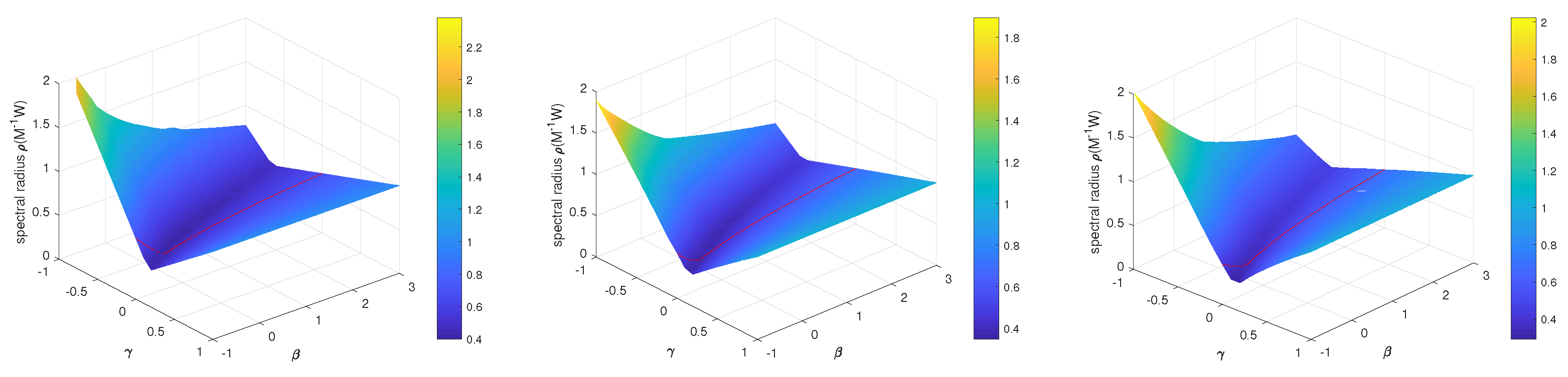For an iterative algorithm, a smaller spectral radius means a faster convergence speed and a better convergence performance. Since this study had three tuning parameters, it was necessary to first fix the value of one tuning parameter before analyzing the convergence effect of the algorithm. In Figure 2, due to space limitations, we only selected three representative $\alpha$ values as $\alpha =0$, $\alpha =0.5$, and $\alpha =1$, since in the previous text we have ${\alpha }_j\in [0,1]$.

Figure 2 displays the spectral radius $\rho \left(M^{-1}W\right)$ when $\beta$, $\gamma$ take different values and $\alpha =0,0.5,$ 1, respectively. The red line represents $\gamma =0$, which is the spectral radius of algorithm (5). In Figure 3, the lowest valley of the surface, which has the smallest spectral radius, is significantly lower than the red curve. This means that when the values of $\alpha$ and $\beta$ are the same as those of algorithm (5), through selecting the appropriate relaxation parameter $\gamma$, algorithm (8) always yields a smaller spectral radius.

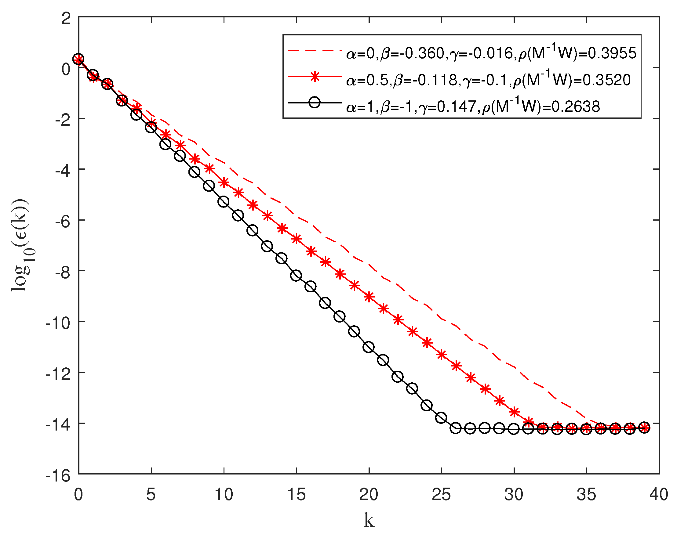
We found the optimal parameters of $\beta$ and $\gamma$ in Figure 2, when $\alpha =0,0.5,$ and 1, respectively, and presented the convergence curves for these three sets of parameters in Figure 3. It is worth mentioning that when the value of $\alpha$ was fixed to 1, by adjusting the value of the parameter $\gamma$, we obtained many spectral radii around 0.26. Algorithm (5) proposed in [25] obtained the minimum spectral radius around approximately 0.31. Obviously, as the parameters changed, algorithm (8) could achieve a better convergence performance.

5. Conclusions

In this article, a novel implicit iterative algorithm for solving continuous stochastic Lyapunov equations is presented via SOR iteration. And the up-to-date information of the solution is utilized to be the latest estimates of the unknown matrices. This method includes three parameters. When proper parameters are chosen, the convergence performance can be greatly improved. Furthermore, the convergence properties are analyzed in detail. Based on the method proposed in [25], we added a parameter to improve the convergence of the algorithm. We always obtained a faster convergence rate by selecting a proper parameter $\gamma$ with the Matlab function. Finally, a numerical example is employed to illustrate that algorithm (8) has a better convergence performance than algorithm (5) proposed in [25].