Analysis of a Predictive Mathematical Model of Weather Changes Based on Neural Networks

Abstract

In this paper, we investigate mathematical models of meteorological forecasting based on the work of neural networks, which allow us to calculate presumptive meteorological parameters of the desired location on the basis of previous meteorological data. A new method of grouping neural networks to obtain a more accurate output result is proposed. An algorithm is presented, based on which the most accurate meteorological forecast was obtained based on the results of the study. This algorithm can be used in a wide range of situations, such as obtaining data for the operation of equipment in a given location and studying meteorological parameters of the location. To build this model, we used data obtained from personal weather stations of the Weather Underground company and the US National Digital Forecast Database (NDFD). Also, a Google remote learning machine was used to compare the results with existing products on the market. The algorithm for building the forecast model covered several locations across the US in order to compare its performance in different weather zones. Different methods of training the machine to produce the most effective weather forecast result were also considered.

1. Introduction

One of the most widespread problems with providing scientific, industrial, and other human activities has been and remains the problem of obtaining information about the environment at the required time [1]. This problem becomes especially important for the support of technical systems (TSs) dependent on meteorological conditions and operating in an autonomous mode. Their parameters cannot be calibrated depending on the meteorological conditions at a certain moment, which makes it necessary to solve the problem of predicting meteorological conditions over a long period of time [2,3,4]. While predicting values for single-parameter technical systems (SPTs) does not pose special problems, multi-parameter technical systems (MTSs) require a thoughtful approach to creating an algorithm for building a predictive model, which makes this problem very relevant.

The problem of obtaining information about the environment and weather forecasting is of great importance for various spheres of human activity. Scientific research, industrial operations, agriculture, urban planning, tourism, and many other sectors require accurate and up-to-date information on weather conditions, climatic changes, and environmental conditions [5,6,7,8].

In the past, environmental information was based mainly on observations and data that were obtained from radio meteorological stations, satellites, sensors, and other devices. Nevertheless, this approach has its limitations due to the large amount of data, the complexity of data processing, and limitations in space and time [9,10].

Due to the development of neural networks and machine learning, new approaches to analysing and predicting weather and environmental conditions have become possible. Neural networks can process large amounts of data and detect complex patterns in weather events, the climate, and other aspects of the environment. They are able to use these patterns to create predictive models that can predict weather and other factors with high accuracy. The application of neural networks in the field of weather and hydrometeorology can improve the quality of forecasts and provide more accurate and reliable data about weather conditions. Neural networks are able to take into account complex interactions between different factors, such as temperature, atmospheric pressure, humidity, and wind, which allows us to obtain more accurate weather forecasts for short and long periods of time [11,12,13].

In addition to weather forecasting, neural networks can be used to analyse and predict other aspects of the environment, such as air pollution, water quality, vegetation, and ecosystem health. This enables informed decision-making in environmental protection, resource management, and other fields of endeavour where environmental information is an important factor. Determining and predicting weather using neural networks require a large amount of data for training and tuning models. Therefore, it is important to create high-quality datasets that include information on past weather events as well as data collected in real time. In addition, machine learning algorithms and neural networks need to be further developed and improved to achieve more accurate and reliable results. Therefore, the application of neural networks in analysing and forecasting weather and the environment makes it possible to solve complex problems related to the acquisition and processing of information in various spheres of human activity. This increases not only the efficiency of scientific and production processes, but also contributes to environmental conservation and informed decision-making in the field of sustainable development [14,15,16,17].

At the moment, various methods and means of obtaining and predicting meteorological data at the desired location of their parameters are known [18,19,20,21], including the following:

• The study of weather phenomena at the current location using physical laws and the Weather Research & Forecasting Model available at https://www.mmm.ucar.edu/models/wrf (accessed on 1 December 2023).
• Investigation of weather conditions by means of mathematical transformations of data received from the probes.
• The use of radar and satellite observations to obtain meteorological information. Radars and satellites can provide data on wind speed, temperature, atmospheric pressure, humidity, and other parameters using a variety of sensors and instruments.
• Application of meteorological balloons and aerological probes that are released into the atmosphere and equipped with meteorological instruments to measure vertical profiles of temperature, humidity, pressure, and wind speed. The obtained data help in weather forecasting and analysing weather conditions.
• The use of a network of meteorological stations located at various locations. These stations have meteorological instruments that continuously monitor and record data on weather conditions, such as temperature, humidity, pressure, and precipitation. The information from these stations helps in forecasting and analysing the weather at the location.
• Utilization of computer weather prediction models that are used to analyse and forecast meteorological data. These models take into account the physical laws of the atmosphere, data from meteorological observations, and other parameters to create forecasts of future weather conditions.
• Usage of remote sensing, such as LIDAR (laser sensing), and infrared sensing to measure atmospheric parameters and obtain weather data. These technologies are based on the analysis of reflected or emitted radiation and can measure temperature, humidity, cloud cover, and other weather characteristics at the desired location.

All these methods and tools are used together to acquire and forecast meteorological data at a given location, which is essential for weather forecasting and the planning of agricultural and urban activities, including safety measures and protection against weather disasters.

The current number of solutions to the problem of building meteorological forecast models and analysing them is staggering. One of the most successful, but at the same time most costly, solutions is the solution provided by Weather Research & Forecasting, which is reduced to the construction of a mathematical model of physical phenomena and, based on the current data, the application of a certain location. However, this approach rarely gives accurate results because it requires a huge number of resources for the solution and constant calculations taking into account the changing parameters of the system. Such a solution also demands the same construction of models for neighbouring regions, which increases the cost of accurate forecasting exponentially, and also does not take into account the essential factors.

Neural networks use one of the most promising methods of MTS forecasting, which is mathematical extrapolation, as this method is based only on the statistical analysis of data [22,23,24]. The drawback of this approach is the impossibility of extrapolating the further development of the process for a long time interval. For this purpose, patterns between input and output values are built, relying on training data. In the case of meteorological forecasting, such data are previous observations collected by the personal weather stations (PWSs).

This paper uses a learning paradigm in which a finite number of neural networks are trained based on the same data to obtain the desired result. This paradigm is called grouping neural networks [25,26,27,28].

The purpose of this study is to describe, analyse, and compare an algorithm for building a predictive model for an MTS for a particular location using the example of data obtained from personal weather stations for certain regions using self-learning machines. The structure of the paper is as follows. The introduction presents the relevance and scientific novelty of the analysis of the predictive mathematical model of weather changes based on neural networks. The second section analyses the structure and application of artificial neural networks. In the third section, the mathematical models of the used neural networks are given. The fourth section describes the mathematical model of the grouping of neural networks proposed for weather forecasts. The fifth section gives an overview of the performance results of the considered mathematical models. The sixth section presents the main conclusions of this work.

2. Analysing the Application of Artificial Neural Networks

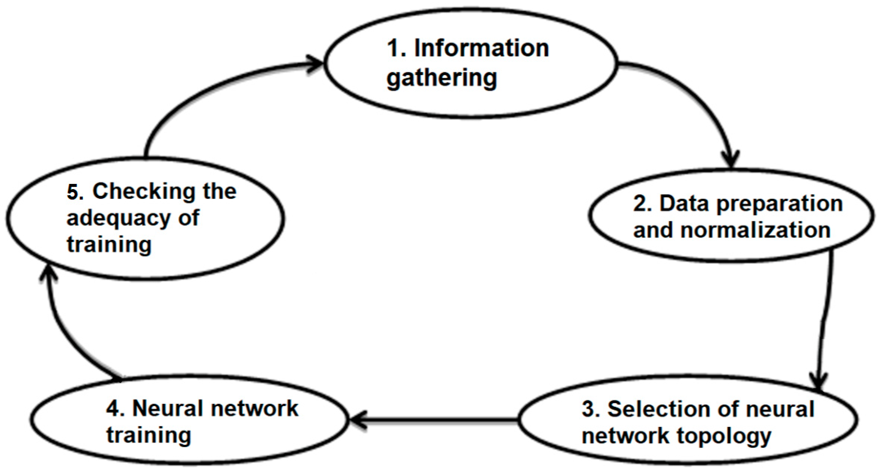
2.1. Stages of Neural Network Construction

When building a neural network, several stages can be distinguished, which can be described in general terms as follows:

-

Defining goals and objectives;

-

Data collection;

-

Data preprocessing;

-

Selection of the neural network architecture;

-

Determination of hyperparameters;

-

Training the network;

-

Model evaluation and tuning;

-

Model development and optimisation.

Each of these stages has its own peculiarities and may require additional actions and experiments to achieve the desired result. To summarise, the main stages of a neural network’s construction are shown in Figure 1.

The first step is to collect weather data. The second step is to normalise and discard corrupted data obtained from Weather Underground and the US National Digital Forecast Database. The normalisation process depends entirely on the choice of topology in the previous step; for example, for RBFN, it is necessary to generate the data in such a way that the training data contain the correct answer.

At the third stage, a mathematical model is selected to build functional dependencies between input and output data to obtain the required result. In this paper, three topologies are considered (D-PNN, RBFN, and MLPN). A new one is also proposed (the grouping method of neural networks).

At the fourth stage, the neural network is trained by feeding pronormalised data to the inputs of the mathematical model. The neural network builds functional dependencies between the data. Finally, the output is a function of the dependence of input and output values in a certain training dataset.

At the fifth stage, the obtained model is checked in terms of accuracy and adequacy. In forecasting, it is necessary to accurately establish the concept of the necessary accuracy of the result. In this paper, the model is considered adequate when its forecast accuracy is 10%, and the accuracy score is calculated as the percentage ratio between the data obtained by the model and the real data.

2.2. Improving the Prediction Accuracy of Neural Networks

Increasing the prediction accuracy of neural networks is an important goal in the field of machine learning, and various approaches and techniques have been used to achieve this goal. Furthermore, ways to improve the prediction accuracy of neural networks have been formulated and proposed, including the following:

-

Increasing the training sample size: A large amount of diverse data can help a neural network learn a wider range of patterns and improve generalisability. This may involve collecting additional data, augmenting existing data, or using generative modelling techniques to create new samples [29,30,31].

-

Improving data quality: Data quality is also important. Data preprocessing should be done to eliminate noise, outliers, missing values, and other problems. In addition, methods can be applied to eliminate class imbalance or sampling imbalance problems.

-

Fitting the network architecture: Choosing the right neural network architecture plays an important role in achieving high prediction accuracy. By using techniques such as hyperparameter search or optimisation by automatic machine learning, different network configurations can be explored, including the number of layers, the number of neurons in each layer, and activation functions.

-

Model regularising: Regularisation techniques can help to control overfitting and generalise the model better to new data. This includes methods such as L1 or L2 regularisation, neuron or layer dropout, and data dimensionality reduction techniques, such as principal component analysis (PCA) and stochastic neighbour embedding with t-distribution (t-SNE).

-

Using pretraining: Pretraining can be useful, especially when there are not enough labelled data available. One can use pretrained models using large unlabelled datasets (e.g., autoencoders or generative models) and then pretrain them based on smaller labelled datasets for a specific task.

-

Combining models: Sometimes, combining multiple models or using ensembles of models can significantly improve the forecast accuracy. This can be done by combining forecasts from several models or by using stacking or bagging techniques.

-

Hyperparameter tuning: The hyperparameters of a model also affect its prediction accuracy. Optimisation techniques, such as grid search or random search, can be used to find optimal values for the hyperparameters.

-

Improving the learning process: Applying various optimisation techniques, such as stochastic gradient descent with momentum (SGD with momentum), Adam’s method, and early stopping, can help to train the neural network more efficiently and stably.

Figure 2 shows the increase in neural network prediction accuracy using generalised data from the ImageNet Large Scale Visual Recognition Challenge (ILSVRC) project [32].

The top-five error rate indicates the percentage of test cases (Figure 2b) where the correct class was not among the top five predicted classes. For instance, if a test image features a Persian cat and the top five predicted classes, ranked from highest to lowest probability, are (Pomeranian (0.4), Mongoose (0.25), Dingo (0.15), Persian cat (0.1), and Tabby cat (0.02)), it is still considered accurate because the real class is within the top five predictions. With ImageNet’s 1000 classes, achieving a low error rate in the top five predictions is challenging [33].

Modern artificial neural networks can be divided into simple and complex (perceptrons) depending on the number of neuron layers (one or more). They are also divided into direct and recurrent networks [34,35,36].

Direct neural networks are used to send the signal from the input to the output in a straight line, like a train on a track. Recurrent ones allow for the possibility that the resulting intermediate value can be sent back to the input again and go through the neural network from the beginning. The biological brain is a recurrent network, which is the reason why it is almost impossible to understand how it works.

Each neural network is a data analysis system that is very powerful and accurate but requires special tuning (training). Moreover, taking into account the self-learning capacity of a neural network, its tuning is not reduced to setting specific parameters according to which it will work. The principle of training is quite different:

-

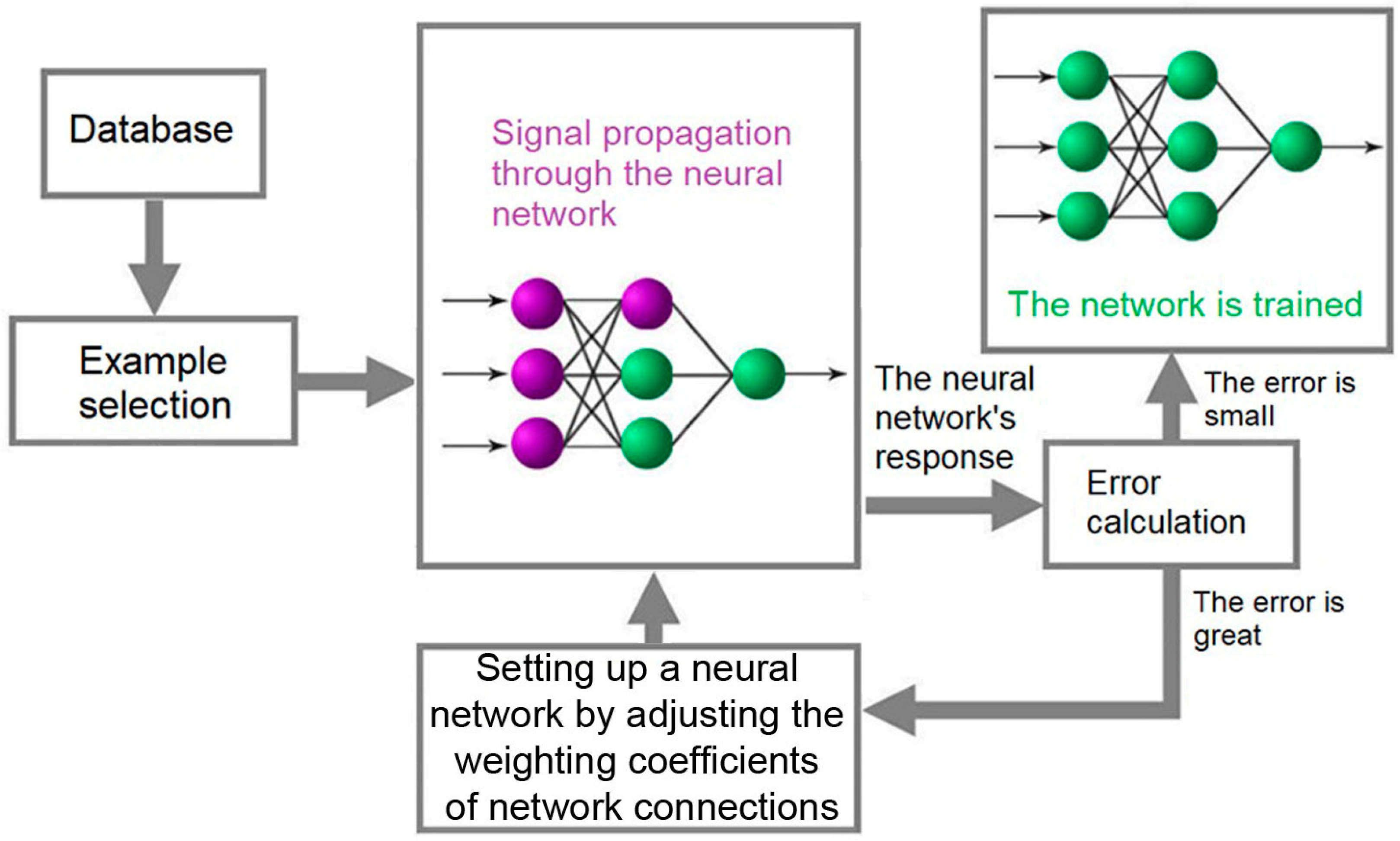
A certain value is given to the input.

-

It is known in advance what value should be at the output.

-

In case the output value is different from the desired value, the network is adjusted until the difference is minimised [37].

The second variant of neural network training is the so-called method of error backpropagation, in which the value obtained at the output, if it differs from the initial one, is transmitted back through the same neurons through which it came to the output. In the process of transmission, the weights of these neurons are increased or decreased. Then, a new attempt follows, and so on until the result becomes optimal. Figure 3 shows the general scheme of the neural network training process proposed for predicting weather changes.

3. Mathematical Models of the Used Neural Networks

The first neural network is based on the solution of the differential polynomial (the differential polynomial neural network (D-PNN). The D-PNN describes functional dependencies of input parameters and their properties, which are often used for forecasting, analysing time series, and revealing hidden relationships in data [38,39,40]. This is achieved by templating the dependencies between the data. The main idea of the D-PNN is the approximation of functions described by differential equations that describe the relationships between the input parameters of the system. The relationships between the data are described similarly to the Kolmogorov–Gabor polynomial presented in 1971 [2]:

$$y=a_0+{\displaystyle \sum _{i=0}^m{\displaystyle \sum _{j=0}^m{a}_{ij}{x}_i{x}_j}}+{\displaystyle \sum _{i=0}^m{\displaystyle \sum _{j=0}^m{\displaystyle \sum _{k=0}^m{a}_{ijk}{x}_i{x}_j}}}{x}_k+\dots ,$$

(1)

where m is the number of variables, x(x₁, x₂, x₃, …) are vectors of input variables, and a(a₁, a₂, a₃, …) are vectors of parameters.

The second neural network is a neural network that uses radial basis functions as activation functions. This network is called the Radial Basis Function Network (RBFN) [41,42,43]. The RFBN is very popular for function approximation, belt series prediction, and classification. In such networks, it is very important to determine the number of neurons in the hidden layer, as it strongly affects the complexity of the network and its generalisation capabilities. In the hidden layer, each neuron has an activating function. The Gaussian function, which has a parameter controlling the behaviour of the function, is the most preferable activation function [34].

$$f(x)=a{e}^{-\frac{{(x-b)}^2}{2c^2}},$$

(2)

where a, b, and c are real numbers.

The third neural network is based on the multilayer perceptron network (MLPN) [35,36,37].

This type of network is known for requiring the presence of the desired result in the training dataset. In our case, it is necessary to supply an additional value that will be the correct result for the input data. In other words, this model relates the input values to their result using historical weather data to predict the weather in the future, which is very important in normalising the data [38].

MLPNs have shown the ability to find approximate solutions for extremely complex problems. In particular, they are a universal function approximator, so they can be successfully used in the construction of regression models. Since classification can be considered as a special case of regression when the output variable is categorical, MLPs can be used to build classifiers [39,40].

Table 1. Comparative characteristics of neural networks.

Principle of Model Construction	Mathematical Description	Input Information	Output Information
D-PNN
Approximation of functions described by differential equations that describe relationships between input parameters of the system	$y=a_0+{\displaystyle \sum _{i=0}^m{\displaystyle \sum _{j=0}^m{a}_{ij}{x}_i{x}_j}}+{\displaystyle \sum _{i=0}^m{\displaystyle \sum _{j=0}^m{\displaystyle \sum _{k=0}^m{a}_{ijk}{x}_i{x}_j}}}{x}_k+\dots$	x(1), x(2), x(3), x(4) … x(n)	x(n + 1)
RBFN
Approximation of the unknown solution by means of functions of a special kind, whose arguments are distant	$y_i(t)=w_{i0}+{\displaystyle \sum _{j=1}^{n_k}{\lambda }_{ij}vl(t)}+{\displaystyle \sum _{j=1}^{n_k}\phi (‖v(t)-c_j(t)‖})$	x(1), x(2), x(3), x(4) … x(n)	x(n + 1)
MLPN
Approximation of the unknown solution using nonlinear functions	$y_i(t)=\varphi ({\displaystyle \sum _{j=1}^n{w}_{ij}{x}_j^k+b_i})$	x(1), x(2), x(3), x(4) … x(n)	x(n + 1)

summarises the comparative performance of the neural networks proposed for weather forecasting.

4. Description of the Mathematical Model of Neural Network Grouping

Neural network grouping, also known as a neural network ensemble or a neural network committee, is a technique in which multiple independent neural networks are trained on the same task in order to improve the prediction quality or system reliability [41,42,43].

The application of neural network clustering has several advantages. First, different neural networks can capture different aspects of the data or extract different characteristics. By combining the predictions of these neural networks, the diverse aspects of the data can be taken into account and the generalisability of the model can be improved. Second, grouping neural networks can help with robustness in terms of noise and outliers. If one neural network makes an error using certain examples, other neural networks can compensate for this error and improve the overall prediction accuracy [44,45,46,47].

The grouping of neural networks can be implemented in various ways:

-

Bagging: This method involves training a set of independent neural networks on subsets of training data obtained by selecting bootstrap examples. The predictions from each neural network are then combined, for example, by majority voting or averaging.

-

Boosting: Unlike bagging, boosting builds a sequence of neural networks, each of which learns to correct the errors of previous networks. At each iteration, the weights of the samples are adjusted to focus on the examples where the previous networks made a mistake. Hence, subsequent neural networks focus on complex and poorly classified examples [48].

-

Stacking: This method is used when the predictions of several neural networks become inputs to another model (a meta-model) that produces the final prediction. In this way, the meta-model is trained to combine and utilise the predictions of different neural networks to produce the best overall result.

Each of these approaches has its own characteristics and is suitable for different scenarios and tasks. The choice of a particular neural network clustering method depends on data characteristics, the required accuracy, computational resources, and other factors. Neural network clustering is a powerful tool used to improve the prediction accuracy and increase the confidence in decision-making. This method is actively used in various fields including computer vision, natural language processing, and speech recognition [49].

Grouping neural networks can be used to predict weather parameters, such as temperature, humidity, and wind speed. This is an important task that helps with planning and decision-making in various fields including agriculture, energy, urban planning, and tourism. One way of applying neural network grouping for weather forecasting is by using the bagging method. In this case, different neural networks are trained on different subsets of the original data with different characteristics (e.g., different time intervals and geographical areas). The forecasts from each neural network are then combined to produce the final weather forecast. This approach can help to account for different features and nuances of weather conditions in different areas [50,51,52].

When applying neural network boosting, a sequence of neural networks learns to predict weather parameters by correcting the errors of previous neural networks. At each iteration, the sample weights or errors of the previous networks are used to emphasise areas where the previous neural networks made an error. In this way, more complex and difficult-to-predict situations can be handled by subsequent neural networks. When neural network stacking is applied to weather forecasting, forecasts from multiple neural networks become inputs to a meta-model that produces the final weather forecast. The meta-model is trained to combine and utilise the forecasts from different neural networks to produce the best overall result [53,54].

An important aspect in weather forecasting is the use of various input features, such as data from weather stations, satellite observations, geographical data, and historical data. Grouping neural networks allows us to combine information from these different sources, which can improve the quality and accuracy of forecasts [55].

All these methods of grouping neural networks for weather forecasting require large amounts of data and computational resources. In addition, it is important to carefully select the structure and parameters of neural networks and train them on a sufficient amount of diverse data to achieve good results [56,57].

The development of more powerful computing resources and the advancement of deep learning have made grouping neural networks increasingly popular and successful in the field of weather forecasting. However, it is always necessary to consider the nature of the complexity of weather processes and the limitations of modelling. Weather forecasts by their nature remain tentative and there remains the possibility that an error will appear in the result, especially in the case of long-term forecasts.

In view of this, neural network grouping is defined by an approach to building a self-learning machine in which a finite number of neural networks is trained to solve the same task. This approach originates from a paper by Hansen and Salamon [58], which shows that the neural network system can be significantly improved by the grouping approach, which means that the predictions produced by such a machine are much more accurate. In general, the grouping of neural networks can be divided into two steps: training several neural networks and then combining and processing the predictions of each. The result of such a system is the averaged value of the outputs of each neural network separately, combined with a function describing the comparative deviation of values obtained at the training stage relative to each other. The results of such systems significantly improve the accuracy of predictions [59,60]. In this paper, a new approach for training these systems will be considered. The weighting coefficients are proportional to the corresponding output values. The essence of the approach is to determine which neural network produces more accurate forecasts. Let us consider an example. One may suppose that there are two neural networks that have to perform a simple classification task. If the input is 1, then the output is 1; if the input is 0, then the output is 0. Let the neural networks’ output be 0.6 and 0.9, respectively, at a certain step. In this case, the second machine receives much more reliable data because 0.9 is closer to 1.

Backpropagation networks set the initial weighting factors randomly to reduce the standard deviation [61,62]. The difference in initial weighting coefficients gives different results. Therefore, grouping neural networks integrates these independent networks to improve the generalisation ability. This method also guarantees an increase in accuracy in terms of a standard deviation [63,64,65,66].

In this paper, we propose a grouping of nonlinear leading networks created using a constructive algorithm. In constructive algorithms, the number of neurons in hidden layers is initially small and then gradually increases. Hence, in constructive algorithms, the skills acquired by the network before increasing the number of neurons are preserved.

Constructive algorithms differ in their rules for setting parameter values in the new neurons added to the network:

-

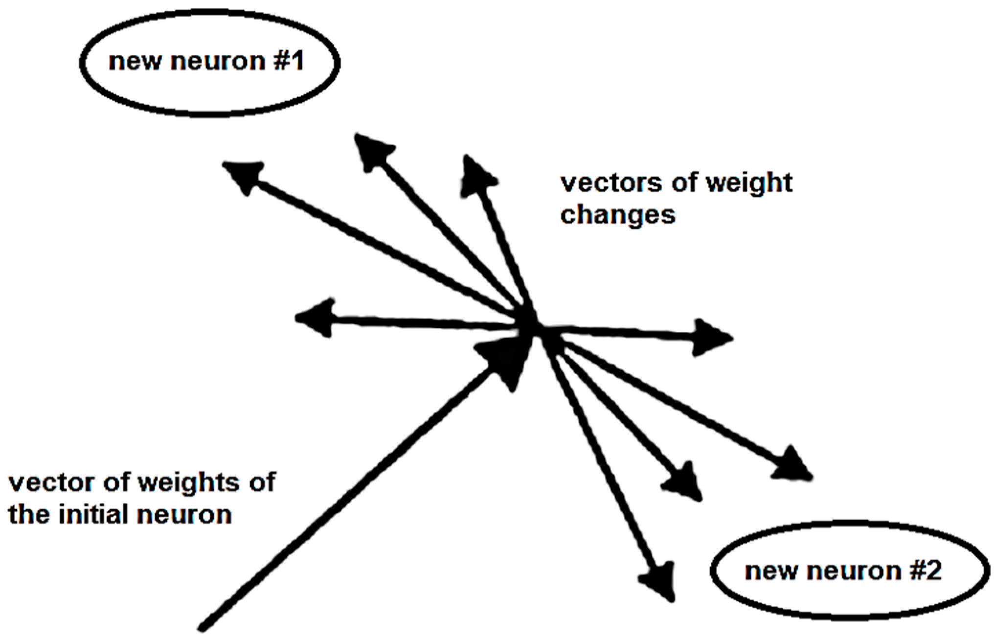
Parameter values are random numbers from a given range;

-

Values of synaptic weights of the new neuron are determined by splitting one of the old neurons.

The first rule does not require significant computation, but its use leads to an increase in the value of the error function after each addition of a new neuron. As a result of the random assignment of parameter values of new neurons, a redundancy in the number of hidden layer neurons may appear. Neuron splitting is devoid of these two disadvantages. The essence of the splitting algorithm is illustrated in Figure 4.

Figure 4 shows the vector of weights of the hidden layer neuron at some training step and the vectors of weight changes corresponding to individual training examples. The change vectors have two preferential directions and form a region in space that is significantly different from the spherical one. The essence of the algorithm is to identify and split such neurons. As a result of splitting, there are two neurons instead of the one initial neuron in the network. The first of these neurons has a vector of weights, which is the sum of the vector of weights of the original neuron, and vectors of changes in the weights of one of the preferential directions. The summation of the vectors of weight changes in the other preferential direction and the vector of weights of the original neuron results in the synaptic weights of the second new neuron [64].

It is necessary to split neurons whose change vectors have two preferential directions because the presence of such neurons leads to oscillations during training by backpropagation. When training the method with an integral error function, the presence of such neurons leads to a hit in the local minimum with a large error value.

The splitting algorithm includes the construction of a covariance matrix of vectors of changes in synaptic weights and the calculation of eigenvectors and eigenvalues of the obtained matrix using the iterative Oja algorithm, according to which stochastic gradient lifting and Gramm–Schmidt orthogonalisation are performed [65].

It is necessary to consider a single neural network that is trained on some dataset. Let x be the input vector that appears for the first time in this network and d be the desired outcome. Values x and d represent the realisation of a random vector X and a random variable D, respectively. Let F(x) be the input–output function realised using the network. Then,

E_D [(F(x) − E[D|X = x])D²] = B_D (F(x)) + V_D (F(x)),

(3)

where E[D|X = x] is the mathematical expectation, B_D(F(x)) is the square of the bias

B_D (F(x)) = (E_D [F(x)] − E[D|X = x])²,

(4)

and V_D (F(x)) is the difference:

V_D (F(x)) = E_D [(F(x) − E_D [F(x)])²].

(5)

The expectation E_D on the set D is called the set covering the distribution of all training data, such as input and output values, and the distribution of all initial conditions. There are several ways to individually train a neural network and several ways to group the output data. This paper assumes that the networks have the same configurations, but their training starts from different initial conditions. An average simple grouping is used to combine the outputs of a group of neural networks. Let ψ be the set of all initial conditions and F_I (x) be the average input–output value of the network functions. Then, by analogy with Equation (3), we obtain

E_ψ [(F_I (x) − E[D|X = x])²] = B_ψ (F(x)) + V_ψ (F(x)),

(6)

where B_ψ (F(x)) is the square of the deviation defined by the set ψ:

B_ψ (F(x)) = (E_ψ [F(x)] − E[D|X = x])²

(7)

and V_ψ (F(x)) is the corresponding difference:

V_ψ (F(x)) = E_ψ [(E_I (x)E_ψ [F(x)])²].

(8)

The mathematical expectation E_ψ is taken for the set ψ.

From the definition of set D, we can think of it as the set of initial conditions ψ and the remaining set is denoted by D′. By analogy with Equation (3), we obtain:

E_D′ [(F_I (x) − E[D|X = x])²] = B_D′ (E_I (x)) + V_D′ (F(x)),

(9)

where B_D′ (F_I (x)) is the square of the deviation defined by the set D′:

B_D′ (F_I (x) = (E_D′ [E_I (x)] − E[D|X = x])²

(10)

and V_D′ (F_I (x)) is the corresponding difference:

V_D′ = E_D′ [(E_I (x) − E_D′ [E_I (x)])²].

(11)

From the definition of sets D, ψ, and D′, it is obvious that:

E_D′ [F_I (x)] = E_D [F(x)].

(12)

It follows that Equation (10) can be rewritten in an equivalent form:

V_D′ (F_I (x)) = (E_D [F(x)] − E[D|X = x])² = B_D (F(x)).

(13)

Having the difference V_D′ (F_I (x)) from Equation (11), since the difference in a random variable is equivalent to the RMS value of a random variable, let us subtract its square of deviation:

V_D′ (F_I (x)) = E_D′ [(F(x))²] − (E_D′ [F(x)])² = E_D′ [(F(x))]

(14)

or

V_D (F_I (x)) = E_D [(F(x))²] − (E_D [F(x)])².

(15)

It is worth considering that the RMS value of function F(x) on set D must be greater than or equal to the RMS value of function F_I (x) on set D′.

E_D [(F(x))²] ≥ E_D′ [(F_I (x))].

(16)

Provided that there are Equations (14) and (15), we have:

V_D′ (F_I (x)) ≤ V_D (F(x)).

(17)

Hence, based on Equations (13) and (17), two conclusions can be drawn:

• The bias of function F_I (x) referring to multiple classification systems is exactly the same as the bias of function F(x) referring to a single neural network.
• The difference in function F_I (x) is smaller than that in function F(x).

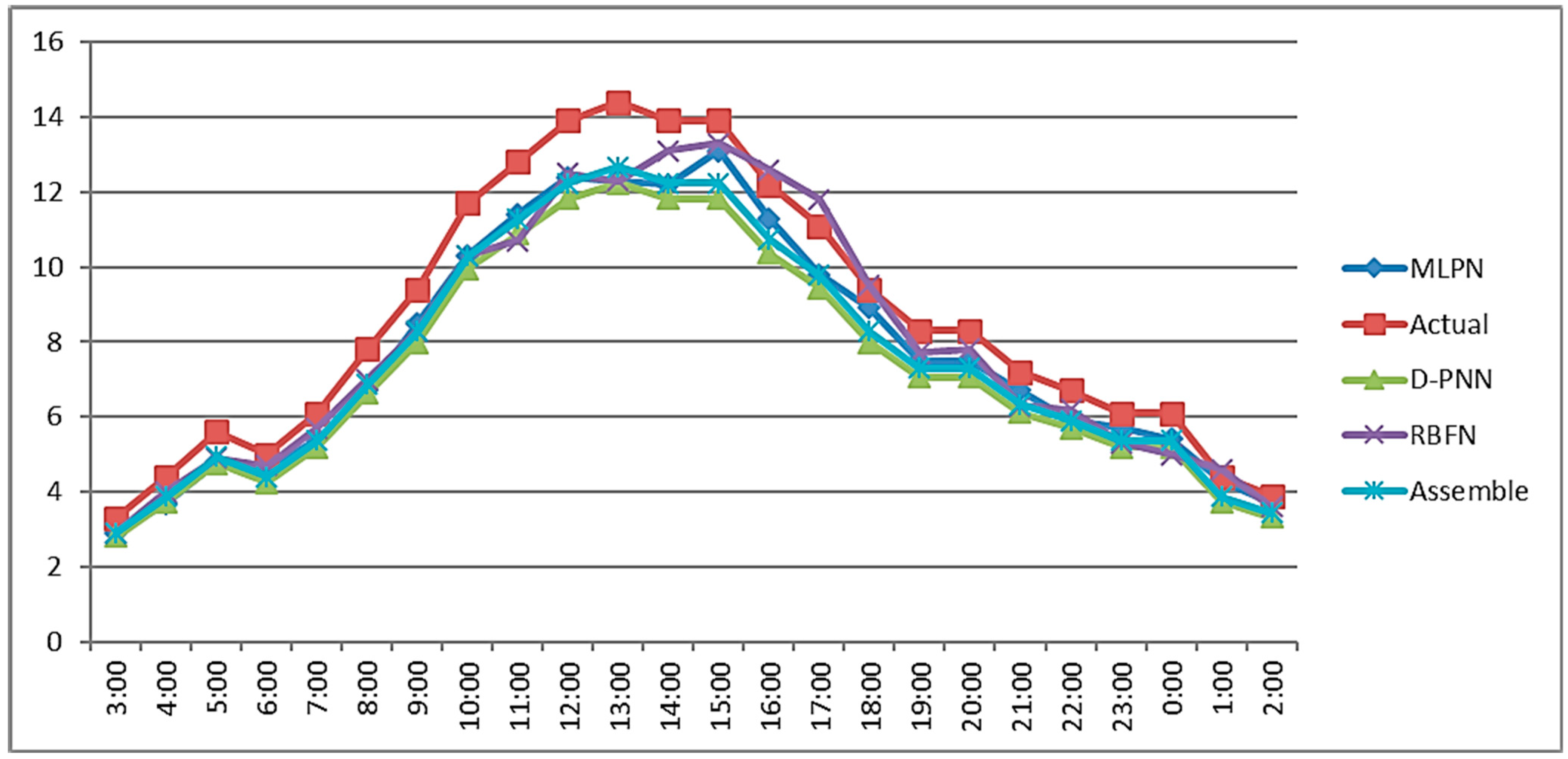
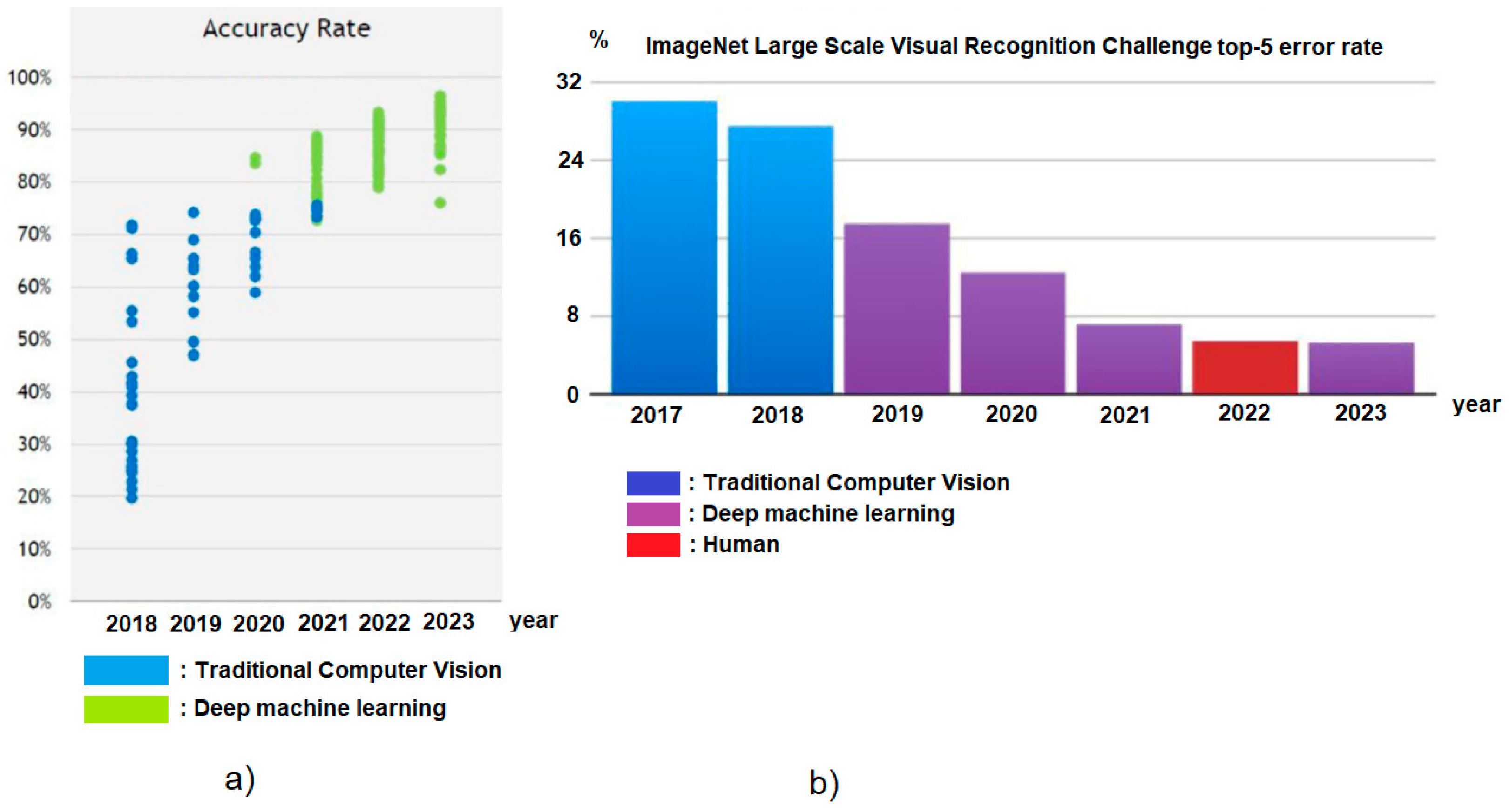
5. Review of the Results of the Considered Mathematical Models

The grouping of linear neural networks has shown improved performance with respect to individual networks. This paper presents the grouping of nonlinear anticipatory networks generated by a constructive algorithm. A similar approach has been applied to the previously discussed D-PNN, RBGN, and MLP.

Statistically, data from Weather Underground personal weather stations and the US National Digital Forecast Database (NDFD) were used to build this model. In addition, Google’s remote learning machine was used to compare the results with existing products on the market.

As a result, the input parameters were historical data obtained from the PWS, and the result of training is a function of the dependence of these parameters on each other. Then, when entering sufficient data in the request for a forecast into the future, we will obtain the data we need. In order to build a forecast based on the above-mentioned mathematical models, we need to arrange the obtained data in the form of an array of enumerated parameters (

Table 2. Example of input data for training.

Temp	City	Daytime	Day_of_Year	Year	Humidity%	Wind Speed kph	Pressure in mBar	Weather Conditions
13.2	1	3	1	2022	18	6	1300	3
14.6	1	4	1	2022	19	7	1150	4
…	…	…	…	…	…	…	…	…

).

In this case, since the model operates using numerical data, cities and weather descriptions were assigned specific indices, e.g., 1 in the city column means Los Angeles. In this study, several training methods were applied by manipulating the input values.

Table 3. Average deviations of predicted temperature values.

Time of Year	Assemble	D-PNN	RBFN	MLPN
Winter	12%	18%	15%	16%
Spring	10%	16%	14%	13%
Summer	8%	14%	16%	11%
Autumn	9%	13%	16%	12%

shows the average deviations of the predicted temperature values.

Let us determine how the models work for different seasons. For this purpose, we enter data for 5 years and compare the obtained data with real values for different periods (0:00–23:00 on 1 January 2022, 0:00–23:00 on 1 April 2022, 0:00–23:00 on 1 July 2022, and 0:00–23:00 on 1 October 2022). Figure 5 shows the predicted air temperature values obtained by each method and the grouping method for 1 January 2022.

When building the forecasting system, its main parameters were determined (forecast horizon, forecast period, and forecast interval). The forecast period is the basic unit of time for which the forecast is formed. The forecast horizon is the number of time periods in the future that the forecast covers. For example, there is a forecast for 10 weeks into the future with data for each week. In this case, the period is one week and the horizon is ten weeks. The forecast interval is the frequency with which a new forecast is generated. Usually, the forecast interval coincides with the forecast period. In this case, the forecast is revised each period using the last period’s claim and other current information as a baseline for the revised forecast. In our case, the forecast theoretical horizon is 1 year.

This work presents a grouping of nonlinear leading networks created using a constructive algorithm. A similar approach was applied to the previously considered D-PNN, RBGN, and MLP. Therefore, the created method of neural network clustering has higher accuracy in all seasons and has an acceptable accuracy of 91%. The pro-forecast accuracy of the other linear neural networks showed the following results of maximum–maximum error: for MLPN it is 13%, for D-PNN it is 15%, and for RBFN it is 11%. The computation time required to obtain a monthly forecast is 4 min. So, predicting the meteorological forecast of temperature changes for a year would take 48 min. Hence, it is possible to realise a forecasting model in a real-time system.

The forecast quality of the weather neural network model has increased by about 2 percent in the last two years (2021–2022).

Table 4. Ranking of temperature predictive models in 2021–2022. Forecast accuracy at 180 h.

№	Country	Accuracy Years 2021/2022, %
		Assemble	D-PNN	RBFN	MLPN
1	USA	89.1/91.4	75.65/77.3	79.21/80.99	77.4/79.2
2	Canada	87.3/90.1	73.9/76.5	77.43/80.1	75.6/78.3
3	Europe	88.7/91.6	74.8/77.35	78.32/80.99	76.5/79.2
4	UK	89.4/90.0	75.65/76.5	79.21/80.1	77.4/78.3
5	Australia	87.2/90.3	73.95/76.5	77.43/80.1	75.6/78.3
6	Germany	88.8/90.7	74.8/76.5	78.32/80.1	76.5/78.3
7	Japan	86.2/88.0	73.1/74.8	76.54/78.4	74.8/76.6
8	China	87.9/88.2	73.95/74.8	77.43/78.3	75.6/76.6
9	Korea	88.3/90.8	74.8/76.5	78.32/80.1	76.5/78.3
10	Russia	86.5/90.2	73.1/76.5	76.54/80.1	74.8/78.3

shows the rankings of temperature prognostic models in 2021–2022 for different countries, with a forecast accuracy of 180 h. To date, the accuracy of most existing predictive weather models is limited to 120 h, while we managed to increase this forecast period to 180 h.

The neural network grouping method is an approach that combines the forecasts of multiple neural networks to produce a more accurate and stable weather forecast. This method uses an ensemble of neural networks that are trained based on historical weather data and other relevant parameters. One of the key aspects of this method is the use of different training algorithms for each neural network in the ensemble. This can include different neural network architectures, various hyperparameters, and various optimisation algorithms. This approach allows for a variety of models that can better capture the characteristics and complexities of different weather seasons.

To achieve a higher forecast accuracy in all weather seasons, the neural network clustering method can apply the averaging or weighting of the contributions of each neural network. This allows us to smooth out possible errors in individual models and take into account different forecast scenarios for different weather seasons. One of the advantages of the neural network clustering method is its ability to adapt to changes in weather conditions. The ability to train and combine models based on current and updated data allows the method to respond quickly to weather changes and provide high forecast accuracy even in new seasons.

Of course, achieving such forecast accuracies requires the preparation of high-quality data and the careful tuning of parameters. An optimal choice of models, the optimisation of hyperparameters, and the use of a large amount of data allow us to achieve the best results. It should be noted that the neural network clustering method may have the potential for application in other areas requiring accurate forecasting, such as financial markets, transportation systems, and energy. Its ability to combine forecasts from multiple models may be useful for improving the forecast accuracy in other areas as well. In this work, we determined that the neural network clustering method is a powerful tool for weather forecasting that provides higher forecast accuracy in all weather seasons and is able to adapt to changes in weather conditions. The application of this method can lead to more reliable and accurate weather forecasts in different areas and has significant practical application.

Therefore, models built using the proposed neural network grouping method can account for a larger number of dependent variables than that of individual neural models, which ultimately improves their accuracy. The grouping of neural networks is an effective tool for working with satellite data in the form of large amounts of weather data, which was shown by the example of the classification of forecast values of objects (Figure 5). Currently, we are developing clustered weather models for such phenomena as snow, cloudiness, ice, and short-term precipitation forecasting based on the applied method of neural network clustering using satellite data and numerical predictive models. All approaches described in this paper were tested using specially generated datasets by experienced decoding specialists. The current algorithms accepted in real operational practice were also compared. The successful results from testing the models presented in this paper allowed us to implement them in the operations of the Novosibirsk weather centre of SIC “Climat”. There were almost no limitations in applying our model in different locations and weather zones in terms of data, as the proposed model involves the processing of large datasets.

6. Conclusions

In this paper, an algorithm for the construction of meteorological forecast models using a grouping of neural networks was developed and investigated. The algorithm for building a mathematical model for predicting future states of meteorological system parameters based on differential polynomials, radial basis functions, multilayer perceptrons, and groupings of neural networks was considered.

The model built using the proposed method of neural network clustering allowed us to consider a larger number of dependent variables than that of individual neural models, which ultimately improved their accuracy. Clustering neural networks is an effective and promising method for processing meteorological information in the form of large datasets on various weather factors, including snow, cloudiness, ice, and short-term precipitation, based on the applied method of neural network clustering and the creation of numerical prognostic models.

Based on the numerical experiment, it can be concluded that the combination of mathematical modelling and “correct” input data related to weather phenomena can make the meteorological forecast model more accurate. In the future, we will continue to study meteorological forecast models in order to not only improve the order and accuracy of input data but also change the mathematical basis for building the model itself.

References

1. Baldauf, M.; Seifert, A.; Forstner, J.; Majewski, D.; Raschendorfer, M.; Reinhardt, T. Operational convective-scale numerical weather prediction with the COSMO model: Description and sensitivities. Mon. Wea. Rev. 2011, 139, 3887–3905. [Google Scholar] [CrossRef]
2. Brisson, E.; Blahak, U.; Lucas-Picher, P.; Purr, C.; Ahrens, B. Contrasting lightning projection using the lightning potential index adapted in a convection-permitting regional climate model. Clim. Dyn. 2021, 57, 2037–2051. [Google Scholar] [CrossRef]
3. Voitovich, E.V.; Kononenko, R.V.; Konyukhov, V.Y.; Tynchenko, V.; Kukartsev, V.A.; Tynchenko, Y.A. Designing the Optimal Configuration of a Small Power System for Autonomous Power Supply of Weather Station Equipment. Energies 2023, 16, 5046. [Google Scholar] [CrossRef]
4. Kleyko, D.; Rosato, A.; Frady, E.P.; Panella, M.; Sommer, F.T. Perceptron Theory Can Predict the Accuracy of Neural Networks. IEEE Trans. Neural Netw. Learn. Syst. 2023, 1–15. [Google Scholar] [CrossRef] [PubMed]
5. Stephan, K.; Schraff, C. Improvements of the operational latent heat nudging scheme used in COSMO-DE at DWD. COSMO Newsl. 2008, 9, 7–11. [Google Scholar]
6. Steppeler, J.; Doms, G.; Schaettler, U.; Bitzer, H.-W.; Gassmann, A.; Damrath, U.; Gregoric, G. Meso-gamma scale forecasts using the nonhydrostatic model LM. Meteorol. Atmos. Phys. 2003, 82, 75–96. [Google Scholar] [CrossRef]
7. Armenta, M.; Jodoin, P.-M. The Representation Theory of Neural Networks. Mathematics 2021, 9, 3216. [Google Scholar] [CrossRef]
8. Bengio, Y.; Goodfellow, I.; Courville, A. Deep Learning; MIT Press: Cambridge, MA, USA, 2015. [Google Scholar]
9. Meng, L.; Zhang, J. IsoNN: Isomorphic Neural Network for Graph Representation Learning and Classification. arXiv 2019, arXiv:1907.09495. [Google Scholar] [CrossRef]
10. Sorokova, S.N.; Efremenkov, E.A.; Qi, M. Mathematical Modeling the Performance of an Electric Vehicle Considering Various Driving Cycles. Mathematics 2023, 11, 2586. [Google Scholar] [CrossRef]
11. Dozat, T. Incorporating Nesterov momentum into Adam. In Proceedings of the ICLR Workshop, San Juan, Puerto Rico, 2–4 May 2016; Volume 1, pp. 2013–2016. [Google Scholar]
12. Xie, S.; Kirillov, A.; Girshick, R.; He, K. Exploring Randomly Wired Neural Networks for Image Recognition. In Proceedings of the IEEE/CVF International Conference on Computer Vision, Seoul, Republic of Korea, 27 October–2 November 2019. [Google Scholar]
13. He, K.; Zhang, X.; Ren, S.; Sun, J. Delving Deep into Rectifiers: Surpassing Human-level Performance on ImageNet Classification. arXiv 2015, arXiv:1502.01852. Available online: https://arxiv.org/pdf/1502.01852.pdf (accessed on 1 December 2023).
14. Kukartsev, V.V.; Martyushev, N.V.; Kondratiev, V.V.; Klyuev, R.V.; Karlina, A.I. Improvement of Hybrid Electrode Material Synthesis for Energy Accumulators Based on Carbon Nanotubes and Porous Structures. Micromachines 2023, 14, 1288. [Google Scholar] [CrossRef]
15. He, K.; Zhang, X.; Ren, S.; Sun, J. Deep Residual Learning for Image Recognition. In Proceedings of the IEEE Conference on Computer Vision and Pattern Recognition, Las Vegas, NV, USA, 27–30 June 2016; pp. 770–778. [Google Scholar]
16. Kalnay, E. Atmospheric Modelling, Data Assimilation and Predictability; Cambridge University Press: Cambridge, UK, 2003. [Google Scholar]
17. Kazakova, E.; Rozinkina, I.; Chumakov, M. Verification of results of the working technology SNOWE for snow water equivalent and snow density fields determination as initial data for COSMO model. COSMO Newsl. 2016, 16, 25–36. [Google Scholar]
18. Chernykh, N.; Mikhalev, A.; Dmitriev, V.; Tynchenko, V.; Shutkina, E. Comparative Analysis of Existing Measures to Reduce Road Accidents in Western Europe. In Proceedings of the 2023 22nd International Symposium INFOTEH-JAHORINA, INFOTEH, Sarajevo, Bosnia and Herzegovina, 15–17 March 2023. [Google Scholar] [CrossRef]
19. Krasnopolsky, V.M.; Lin, Y. A neural network nonlinear multimodel ensemble to improve precipitation forecasts over continental US. Adv. Meteorol. 2012, 2012, 649450. [Google Scholar] [CrossRef]
20. Marzban, C. A neural network for post-processing model output: ARPS. Mon. Wea. Rev. 2003, 131, 1103–1111. [Google Scholar] [CrossRef]
21. Warner, T.T. Numerical Weather and Climate Prediction; Cambridge University Press: Cambridge, UK, 2010. [Google Scholar]
22. Ye, C.; Zhao, C.; Yang, Y.; Fermuller, C.; Aloimonos, Y. LightNet: A Versatile, Standalone Matlab-based Environment for Deep Learning. arXiv 2016. Available online: https://arxiv.org/pdf/1605.02766.pdf (accessed on 1 December 2023).
23. Zurada, J.M. Introduction to Artificial Neural Systems; PWS: New York, NY, USA, 1992. [Google Scholar]
24. Goyal, M.; Goyal, R.; Lall, B. Learning Activation Functions: A New Paradigm of Understanding Neural Networks. arXiv 2019, arXiv:1906.09529. [Google Scholar]
25. Burgers, G.; Van Leeuwen, P.J.; Evensen, G. Analysis scheme in the ensemble Kalman filter. Mon. Weather. Rev. 1998, 126, 1719–1724. [Google Scholar] [CrossRef]
26. Dey, R.; Chakraborty, S. Convex-hull & DBSCAN clustering to predict future weather. In Proceedings of the 2015 International Conference and Workshop on Computing and Communication (IEMCON), Vancouver, BC, Canada, 15–17 October 2015; pp. 1–8. [Google Scholar] [CrossRef]
27. Saima, H.; Jaafar, J.; Belhaouari, S.; Jillani, T.A. Intelligent methods for weather forecasting: A review. In Proceedings of the 2011 National Postgraduate Conference, Perak, Malaysia, 19–20 September 2011; pp. 1–6. [Google Scholar] [CrossRef]
28. Salman, A.G.; Kanigoro, B.; Heryadi, Y. Weather forecasting using deep learning techniques. In Proceedings of the International Conference on Advanced Computer Science and Information Systems (ICACSIS), Depok, Indonesia, 10–11 October 2015; pp. 281–285. [Google Scholar] [CrossRef]
29. Singh, N.; Chaturvedi, S.; Akhter, S. Weather forecasting using machine learning algorithm. In Proceedings of the 2019 International Conference on Signal Processing and Communication (ICSC), Noida, India, 7–9 March 2019; pp. 171–174. [Google Scholar] [CrossRef]
30. Sela, J.G. The Implementation of the Sigma Pressure Hybrid Coordinate into the GFS. Office Note (National Centers for Environmental Prediction (U.S.)). 2009; p. 461. Available online: https://repository.library.noaa.gov/view/noaa/11401 (accessed on 1 December 2023).
31. Weather Research & Forecasting Model (WRF) Mesoscale & Microscale Meteorology Laboratory. NCAR. Available online: https://www.mmm.ucar.edu/models/wrf (accessed on 1 December 2023).
32. Yonekura, K.; Hattori, H.; Suzuki, T. Short-term local weather forecast using dense weather station by deep neural network. In Proceedings of the IEEE International Conference on Big Data (Big Data), Seattle, WA, USA, 10–13 December 2018; pp. 1683–1690. [Google Scholar] [CrossRef]
33. Bauer, P.; Thorpe, A.; Brunet, G. The quiet revolution of numerical weather prediction. Nature 2015, 525, 47–55. [Google Scholar] [CrossRef]
34. Buschow, S.; Friederichs, P. Local dimension and recurrent circulation patterns in long-term climate simulations. arXiv 2018, 1803, 11255. [Google Scholar] [CrossRef]
35. C3S: ERA5: Fifth Generation of ECMWF Atmospheric Reanalyses of the Global Climate, Copernicus Climate Change Service Climate Data Store (CDS). 2017. Available online: https://cds.climate.copernicus.eu/cdsapp#!/home (accessed on 7 June 2019).
36. Compo, G.P.; Whitaker, J.S.; Sardeshmukh, P.D.; Matsui, N.; Allan, R.J.; Yin, X.; Gleason, B.E.; Vose, R.S.; Rutledge, G.; Bessemoulin, P.; et al. The twentieth century reanalysis project. Q. J. R. Meteor. Soc. 2011, 137, 1–28. [Google Scholar] [CrossRef]
37. Coors, B.; Paul Condurache, A.; Geiger, A. Spherenet: Learning spherical representations for detection and classification in omnidirectional images. In Proceedings of the European Conference on Computer Vision (ECCV), Munich, Germany, 8–14 September 2018; pp. 518–533. [Google Scholar]
38. Dee, D.P.; Uppala, S.M.; Simmons, A.; Berrisford, P.; Poli, P.; Kobayashi, S.; Andrae, U.; Balmaseda, M.; Balsamo, G.; Bauer, P.; et al. The ERA-Interim reanalysis: Configuration and performance of the data assimilation system. Q. J. R. J. R. Meteor. Soc. 2011, 137, 553–597. [Google Scholar] [CrossRef]
39. Dueben, P.D.; Bauer, P. Challenges and design choices for global weather and climate models based on machine learning. Geosci. Model Dev. 2018, 11, 3999–4009. [Google Scholar] [CrossRef]
40. Faranda, D.; Messori, G.; Yiou, P. Dynamical proxies of North Atlantic predictability and extremes. Sci. Rep. 2017, 7, 41278. [Google Scholar] [CrossRef] [PubMed]
41. Faranda, D.; Messori, G.; Vannitsem, S. Attractor dimension of time-averaged climate observables: Insights from a low-order ocean-atmosphere model. Tellus A 2019, 71, 1–11. [Google Scholar] [CrossRef]
42. Fraedrich, K.; Jansen, H.; Kirk, E.; Luksch, U.; Lunkeit, F. The Planet Simulator: Towards a user-friendly model. Meteorol. Z. 2005, 14, 299–304. [Google Scholar] [CrossRef]
43. Freitas, A.C.M.; Freitas, J.M.; Todd, M. Hitting time statistics and extreme value theory. Probab. Theory Rel. 2010, 147, 675–710. [Google Scholar] [CrossRef]
44. Tynchenko, V.; Kurashkin, S.; Murygin, A.; Bocharov, A.; Seregin, Y. Software for optimization of beam output during electron beam welding of thin-walled structures. Procedia Comput. Sci. 2022, 200, 843–851. [Google Scholar] [CrossRef]
45. Kukartsev, V.V.; Tynchenko, V.S.; Bukhtoyarov, V.V.; Wu, X.; Tyncheko, Y.A.; Kukartsev, V.A. Overview of Methods for Enhanced Oil Recovery from Conventional and Unconventional Reservoirs. Energies 2023, 16, 4907. [Google Scholar] [CrossRef]
46. Krasnopolsky, V.M.; Fox-Rabinovitz, M.S. Complex hybrid models combining deterministic and machine learning components for numerical climate modelling and weather prediction. Neural Netw. 2006, 19, 122–134. [Google Scholar] [CrossRef]
47. Filina, O.A.; Sorokova, S.N.; Efremenkov, E.A.; Valuev, D.V.; Qi, M. Stochastic Models and Processing Probabilistic Data for Solving the Problem of Improving the Electric Freight Transport Reliability. Mathematics 2023, 11, 4836. [Google Scholar] [CrossRef]
48. Krasnopolsky, V.M.; Fox-Rabinovitz, M.S.; Belochitski, A.A. Using ensemble of neural networks to learn stochastic convection parameterisations for climate and numerical weather prediction models from data simulated by a cloud resolving model. Adv. Artif. Neural Syst. 2013, 2013, 485913. [Google Scholar] [CrossRef]
49. Lorenz, E.N. Deterministic nonperiodic flow. J. Atmo. Sci. 1963, 20, 130–141. [Google Scholar] [CrossRef]
50. Das, P.; Manikandan, S.; Raghavendra, N. Holomorphic aspects of moduli of representations of quivers. Indian J. Pure Appl. Math. 2019, 50, 549–595. [Google Scholar] [CrossRef]
51. Konyukhov, V.Y.; Oparina, T.A.; Zagorodnii, N.A.; Efremenkov, E.A.; Qi, M. Mathematical Analysis of the Reliability of Modern Trolleybuses and Electric Buses. Mathematics 2023, 11, 3260. [Google Scholar] [CrossRef]
52. Filina, O.A.; Tynchenko, V.S.; Kukartsev, V.A.; Bashmur, K.A.; Pavlov, P.P.; Panfilova, T.A. Increasing the Efficiency of Diagnostics in the Brush-Commutator Assembly of a Direct Current Electric Motor. Energies 2024, 17, 17. [Google Scholar] [CrossRef]
53. Frankle, J.; Carbin, M. The Lottery Ticket Hypothesis: Finding Sparse, Trainable Neural Networks. In Proceedings of the International Conference on Learning Representations, New Orleans, LA, USA, 6–9 May 2019. [Google Scholar]
54. Nooteboom, P.D.; Feng, Q.Y.; López, C.; Hernández-García, E.; Dijkstra, H.A. Using network theory and machine learning to predict El Nino. Earth Syst. Dynam. 2018, 9, 969–983. [Google Scholar] [CrossRef]
55. O’Gorman, P.A.; Dwyer, J.G. Using Machine Learning to Parameterize Moist Convection: Potential for Modeling of Climate, Climate Change, and Extreme Events. J. Adv. Model. Earth Syst. 2018, 10, 2548–2563. [Google Scholar] [CrossRef]
56. Golik, V.I.; Brigida, V.; Kukartsev, V.V.; Tynchenko, Y.A.; Boyko, A.A.; Tynchenko, S.V. Substantiation of Drilling Parameters for Undermined Drainage Boreholes for Increasing Methane Production from Unconventional Coal-Gas Collectors. Energies 2023, 16, 4276. [Google Scholar] [CrossRef]
57. Volneikina, E.; Kukartseva, O.; Menshenin, A.; Tynchenko, V.; Degtyareva, K. Simulation-Dynamic Modeling of Supply Chains Based on Big Data. In Proceedings of the 2023 22nd International Symposium INFOTEH-JAHORINA, INFOTEH 2023, Sarajevo, Bosnia and Herzegovina, 15–17 March 2023. [Google Scholar] [CrossRef]
58. Poli, P.; Hersbach, H.; Dee, D.P.; Berrisford, P.; Simmons, A.J.; Vitart, F.; Laloyaux, P.; Tan, D.G.H.; Peubey, C.; Thépaut, J.-N.; et al. ERA-20C: An Atmospheric Reanalysis of the Twentieth Century. J. Clim. 2016, 29, 4083–4097. [Google Scholar] [CrossRef]
59. Semenova, E.; Tynchenko, V.; Chashchina, S.; Suetin, V.; Stashkevich, A. Using UML to Describe the Development of Software Products Using an Object Approach. In Proceedings of the 2022 IEEE International IOT, Electronics and Mechatronics Conference (IEMTRONICS), Toronto, ON, Canada, 1–4 June 2022. [Google Scholar] [CrossRef]
60. Scher, S. Toward Data-Driven Weather and Climate Forecasting: Approximating a Simple General Circulation Model with Deep Learning. Geophys. Res. Lett. 2018, 45, 12616–12622. [Google Scholar] [CrossRef]
61. Martyushev, N.V.; Malozyomov, B.V.; Sorokova, S.N.; Efremenkov, E.A.; Valuev, D.V.; Qi, M. Review Models and Methods for Determining and Predicting the Reliability of Technical Systems and Transport. Mathematics 2023, 11, 3317. [Google Scholar] [CrossRef]
62. Scher, S. Videos for Weather and climate forecasting with neural networks: Using GCMs with different complexity as studyground. Zenodo 2019. [Google Scholar] [CrossRef]
63. Scher, S. Code and data for Weather and climate forecasting with neural networks: Using GCMs with different complexity as study-ground. Zenodo 2019. [Google Scholar] [CrossRef]
64. Martyushev, N.V.; Malozyomov, B.V.; Kukartsev, V.V.; Gozbenko, V.E.; Konyukhov, V.Y.; Mikhalev, A.S.; Kukartsev, V.A.; Tynchenko, Y.A. Determination of the Reliability of Urban Electric Transport Running Autonomously through Diagnostic Parameters. World Electr. Veh. J. 2023, 14, 334. [Google Scholar] [CrossRef]
65. Scher, S.; Messori, G. Predicting weather forecast uncertainty with machine learning. Q. J. R. Meteor. Soc. 2018, 144, 2830–2841. [Google Scholar] [CrossRef]
66. Schneider, T.; Lan, S.; Stuart, A.; Teixeira, J. Earth System Modeling 2.0: A Blueprint for Models That Learn from Observations and Targeted High-Resolution Simulations. Geophys. Res. Lett. 2017, 44, 12396–12417. [Google Scholar] [CrossRef]
Figure 1. Main stages of a neural network’s construction.
Mathematics 12 00480 g001
Figure 2. Increase in neural network prediction accuracy: (a) accuracy rate and (b) top-5 error rate in the ILSVRC.
Mathematics 12 00480 g002
Figure 3. Schematic diagram of the training process of the weather neural network.
Mathematics 12 00480 g003
Figure 4. Vector of hidden layer neuron weights and changes corresponding to individual training examples.
Mathematics 12 00480 g004
Figure 5. Graph of forecast values obtained by each method as of 1 January 2022.
Mathematics 12 00480 g005