Abstract
The COVID-19 epidemic has required countries to implement different containment strategies to limit its spread, like strict or weakened national lockdown rules and the application of age-stratified vaccine prioritization strategies. These interventions have in turn modified the age-dependent patterns of social contacts. In our recent paper, starting from the available age-structured real data at the national level, we identified, for the Italian case, specific virulence parameters for a two-age-structured COVID-19 epidemic compartmental model (under 60, and 60 years and over) in six different diseases transmission scenarios under concurrently adopted feedback interventions. An interpretation of how each external scenario modifies the age-dependent patterns of social contacts and the spread of COVID-19 disease has been accordingly provided. In this paper, which can be viewed as a sequel to the previous one, we mainly apply the same general methodology therein (involving the same dynamic model) to new data covering the three subsequent additional scenarios: (i) a mitigated coordinated intermittent regional action in conjunction with the II vaccination phase; (ii) a super-attenuated coordinated intermittent regional action in conjunction with the II vaccination phase; and (iii) a last step towards normality in conjunction with the start of the III vaccination phase. As a new contribution, we show how meaningful updated information can be drawn out, once the identification of virulence parameters, characterizing the two age groups within the latest three different phases, is successfully carried out. Nevertheless, differently from our previous paper, the global optimization procedure is carried out here with the number of susceptible individuals in each scenario being left free to change, to account for reinfection and immunity due to vaccination. Not only do the slightly different estimates we obtain for the previous scenarios not impact any of the previous considerations (and thus illustrate the robustness of the procedure), but also, and mainly, the new results provide a meaningful picture of the evolution of social behaviors, along with the goodness of strategic interventions.
Keywords:
COVID-19 epidemic; model identification; parameter estimation; compartmental model; vaccine effects; global optimization MSC:
37M10; 34H05; 37M05; 62P25; 93B30; 91C05; 00A06
1. Introduction
The worldwide reaction to the unprecedented challenges posed by the COVID-19 pandemic has been marked by a diverse array of strategic initiatives and interventions, implemented with the collective goal of not only containing the transmission of the virus but also mitigating the far-reaching impacts it has had on public health, socio-economic structures, and the overall fabric of global societies. Scientific research, particularly that grounded in mathematical models, has played a pivotal role in steering these interventions, providing valuable insights and innovative ideas that have informed decision-making processes and enhanced the effectiveness of public health strategies on a global scale. These proposed strategies have encompassed a spectrum of measures, including widespread lockdown and social distancing protocols [1,2], the promotion and enforcement of mask-wearing, extensive testing, and contact tracing efforts [3,4,5], the rapid development and deployment of vaccines [6,7], and public awareness campaigns [8,9,10].
Moreover, scientific research has been instrumental in comprehending the multifaceted impact of each proposed measure, offering a nuanced understanding from both health and socio-economic perspectives [11,12,13]. This dual assessment has been crucial in shaping a holistic approach, ensuring that interventions not only address the immediate health crisis but also consider the broader implications on societies and economies [14,15,16]. By integrating scientific findings into policy discussions, nations have been better equipped to navigate the intricate balance between safeguarding public health and minimizing socio-economic disruptions, exemplifying a commitment to evidence-based decision-making in the face of this complex global health crisis.
The aspect of utmost significance that has garnered scientific and societal attention for COVID-19 is its mortality rate. Although all age groups have been susceptible to COVID-19 infection, older age groups have faced an elevated risk of severe symptoms and mortality [17,18,19]: the case fatality rate among adults over 60 years has been estimated to be four times higher than that of young adults [20]. This stark reality has prompted a series of studies aimed at understanding how the virus spreads within a population, considering the variations in age distribution. For instance, ref. [21] introduced a compartmental model to predict the number of infected, hospitalized, and deceased individuals in a population divided into 17 age classes, parameterizing it using COVID-19 infection data from Switzerland. Taking a step further in analyzing the virus spread across different age groups, ref. [22] proposed a partial differential equation model, forecasting the disease progression in three countries spanning different continents: the United States of America, the United Arab Emirates, and Algeria. These studies also provided recommendations for interventions based on age including prioritizing vaccination for older individuals and implementing stricter age-dependent social distancing measures.
Italy, being at the forefront of the pandemic’s impact, underwent a series of rigorous measures and interventions to combat the unprecedented challenges posed by the novel coronavirus [2]. In our study [23], we ventured into uncharted territory by pioneering the development of a two-age-structured COVID-19 epidemic model. This model utilizes real data at the national level to discern how the various phases of the pandemic in Italy has changed our typical social behaviors between the elder and the young population. Leveraging available age-structured real data, we uncovered valuable insights into the nuanced relationships between age demographics, social contacts, and the transmission of COVID-19. The model not only offered a comprehensive understanding of the disease dynamics but also facilitated an interpretation of how external scenarios, such as public health interventions and societal behaviors, modified age-dependent patterns of social contacts.
As a logical progression of our earlier work [23], this paper serves as a consequential sequel, in which we not only incorporate new and updated data but also perform the global optimization procedure by leaving the number of susceptible individuals in each scenario free to change, to account for reinfection and vaccination-owing immunity. The present work does not thus present a contribution to the theory of epidemic models, namely, no new model is proposed. Instead, it presents how to use the model of [23] to further interpret reality wisely. Changing the parameter identification procedure generates slightly different estimates for the previous scenarios, which, notably, do not impact any of the previously drawn considerations, thus illustrating the robustness of the procedure and the goodness of our previous results. Through the lens of our two-age-structured model, we aim to provide a nuanced analysis of the dynamic interplay between strategic actions, societal behaviors, and the evolving patterns of COVID-19 transmission. In essence, this paper serves as a bridge between the theoretical constructs of our initial model and the evolving realities of the pandemic. By applying our established framework to fresh sets of data, we seek to unravel the intricate ways in which the implemented interventions have shaped the trajectory of the virus. This effort is not merely an academic exercise; it is a timely exploration of the real-world implications of strategic actions and behavioral adaptations in the ongoing battle against COVID-19.
2. Incorporation of New Data into the Methodology of [23]
2.1. Retrospect
The real data that were analyzed in [23] had been taken from the Italian context, where the following subsequent-in-time different strategies were implemented:
- (a)
- A strict national lockdown rule (scenario a, from 9 March 2020 to 28 April 2020) that removes social contacts in workplaces, schools, markets, and other public areas;
- (b–d)
- A weakened feedback social distancing and contact reduction intervention, which is composed of a weakened lockdown phase (scenario b, from 7 May 2020 to 3 June 2020), a low-distancing phase (scenario c, from 9 June 2020 to 8 September 2020), and a low-distancing + workplace/school-contacts re-activation phase (scenario d, from 15 September 2020 to 27 October 2020), with a progressive release of the population back to their daily routine;
- (e)
- A coordinated intermittent regional action (scenario e, from 7 November 2020 to 29 December 2020), where social distancing measures are put in place or relaxed independently by each region based on the ratio between hospitalized individuals and the specific regional health system capacity;
- (f)
- Direct mRNA-vaccination of subjects—especially the elderly—(scenario f, from 5 January 2021 to 12 May 2021) at highest risk for severe outcomes, along with Vaxzevria vaccination of young subjects within specific occupational categories (to protect subjects at highest risk for severe outcomes indirectly).
2.2. The New Three Subsequent Scenarios
We now identify another three scenarios, characterized by a successive weakening of the rules adopted during lockdown (until the abolition of the mandatory use of masks in public places and hospitals) during the vaccination campaign. The three such scenarios are characterized by:
- (G)
- A mitigated coordinated intermittent regional action in conjunction with the II vaccination phase (scenario G, from 19 May 2021 to 14 July 2021): during this phase, only people with a COVID-19 vaccination certificate (Green Pass) can leave their city of residence, and schools that were teaching online until scenario (f) resume normal operation (in presence);
- (H)
- A super-attenuated coordinated intermittent regional action, without mobility restrictions, where even large events (such as sports competitions, congresses, fairs, private parties) can be held in the regions with a sufficiently low number of cases, in conjunction with the II vaccination phase (scenario H, from 21 July 2021 to 22 September 2021);
- (I)
- The last step towards normality (normal reopening of schools, with the vaccination certificate only mandatory for teachers, complete lifting of the obligation to use face masks, reopening of entertainment activities such as discos and ballrooms) and start of the III vaccination phase (scenario I, from 29 September 2021 to 10 November 2021).
All the data are taken from the official Ministerial website https://www.epicentro.iss.it/coronavirus/aggiornamenti (accessed on 26 September 2023), which report: (i) the cumulative detected cases on a weekly scale, , divided per age (to compute and ); and (ii) the number of recovered people (not divided per age), .
3. Model and Simplifying Assumptions
In this section, for the sake of exhaustiveness, we recall the deterministic compartmental model proposed in [23]. The model was proposed to investigate how different epidemic phases, characterized by different political strategies used to contain the epidemics, affected the age-dependent patterns of social contacts and the spread of COVID-19. It is a natural extension of the classical SIR model in which the fluxes between the susceptible and the infected compartments are assumed to be proportional to the encounter rate. Each compartment is subdivided into different age groups. In order to avoid issues related to the lack of parameter identifiability, modeling and analysis were limited to two age groups. The two age groups correspond to individuals below the age of 60 and those aged 60 and older. As already highlighted in [23], at least four reasons guide the choice of such two groups. 1. Such a division highlights a division of active and retired populations, with different patterns of social interactions leading to different transmission dynamics. 2. Empirical estimates based on population-level data recognize a sharp difference in fatality rates between young and old people. 3. Priority for vaccination in Italy has been given to people older than 60 years. 4. A closer look at the Italian data reveals that this choice leads to a uniform division of the number of COVID-19 cases most uniformly.
We recall that the model aims to identify the parameters in the aforementioned time windows. More specifically, the length of the periods for our model equates, on average, to a couple of months, and always less than 4 months. At the beginning of each time window, moreover, the initial conditions are estimated from the data. In light of this, the following simplifying assumptions are here further specified:
- Aging, reproduction, and natural death have negligible effects so that the variation in the number of susceptible in the time window only depends on infection.
- Infected people cannot be infected another time in the time window.
- Effect of vaccines against infection is negligible in the time window.
The above assumptions limit the maximum length of the time windows; in other words, the model cannot be used to make any forecast on long time windows, since it neglects fundamental characteristics such as aging, reinfection, and vaccination. These assumptions, however, hold in the short time, and aging, becoming susceptible after an infection, or gaining immunity with vaccination are captured by the model at the beginning of the time window at which the estimation of the current susceptible subjects is carried out. The resulting model is accordingly given by:
in which:
- t is the time, measured in days;
- , are the numbers of susceptible and infected for the two age classes, respectively;
- and are the numbers of reported cases for the two age classes;
- is the number of persons who are not quarantined, hospitalized, or dead at time t.
A schematic of the model is proposed in Figure 1, in which each state variable is represented by a node, and the arrows represent the fluxes between the state variables. The parameters , represent the virulence of the virus among the different age classes, while , is the average time for disease identification, and is the rate of asymptomatic infected who recover without being reported. As for the SIR model, an explicit solution to Equation (1) is not available. On the other hand, being a dynamical model, it can provide us with the forward evolution of the time series of the state variables, once an initial condition is given. However, note that the presented model needs the time series of active people, , to be simulated. This series cannot be reconstructed from the state variables, since the number of quarantined, hospitalized, recovered, or dead are not taken into account. As in [23], the scope of this model is not to make a prediction, but just to estimate its parameters to overview people’s reactions, subject to the new three different scenarios.
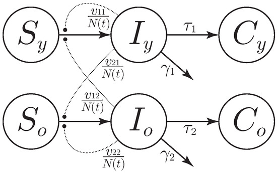
Figure 1.
Schematic of model (1). Each node represents a state variable of the model (, are the numbers of susceptible, infected, and reported cases for the two age classes, respectively), with each arrow representing a flux—proportional to the reported parameter and the departing node value—toward the arriving node. The dotted lines represent nonlinear proportional interactions that also modulate the flux.
4. Estimation of Model Parameters
The methodology proposed in [23] is aimed at identifying the changes in behavior and social interactions between older and young people based on the number of COVID-19 reported cases. The key parameters used to achieve this goal are:
- , characterizing the intra-juvenile virulence;
- , characterizing the juvenile–elder virulence;
- , characterizing the elder–juvenile virulence;
- , characterizing the intra-elder virulence;
- , denoting the average time for disease identification in young subjects;
- , denoting the average time for disease identification in old subjects;
- , representing the young subjects infected at the beginning of the scenario time window;
- , representing the old subjects infected at the beginning of the scenario time window.
The parameters are identified in the new aforementioned scenarios by adapting the procedure proposed in [23], which uses the relationship
representing the number of active people each day, while fitting the model (namely, parameters and initial conditions) to the real data by minimizing a cost function. More specifically, starting from the time window that identifies scenario a, i.e., , , we compute the trajectory of the model
that starts from the initial conditions
Notice that this is different from what was performed in [23], where, for each time window i, the number of susceptible at the beginning of the time window was set to , . As mentioned before, this is done to account for both the reinfection and the immunity against infection that is possibly provided by the vaccination. At last, we compute—as a cost—the relative error between the predicted and the real new daily cases. Finally, to guarantee the continuity of the identified solution, we impose the initial condition of the current scenario (parameters , , , ) to be different from the final condition of the previous one by at most 30%.
The details of such a procedure are provided hereafter. Let , denote the reported cases for the two age classes (the bar-notation specifies the real nature of the data); the new cases reported at time are thus given by , . On the other hand, the new cases predicted—by the model—within the i-th time window come from the last equations of (1), so as to obtain , . Accordingly, the cost associated with the i-th time window is given by
Now, on the basis of the time series of the reported cases for the two age classes, , , and the time series of the recovered people, , the number of active people is computed as
and the model parameters and initial conditions are then determined as solutions—through the fmincon routine in Matlab©—to the optimization problem
that exhibits 90 free parameters (the others being fixed by the equality constraints).
Note that data are collected weekly so that the cost function is computed only at the time for which the data are present and not each day, t. The total number of data we use for our fitting procedure is 198, while the problem of estimation needs at least 90 data points (one for each of the parameters we are estimating). As in [23], a practical identifiability analysis of the parameters around the estimation point confirms that the values we obtained with this procedure can be locally determined from the data we used (the local minimum we have found has no directions on which the cost function does not significantly increase with respect to the parameter variations). Moreover, the obtained estimates turn out to be robust with respect to the hyper-parameters characterizing the optimization method, including the 30% barrier imposed to guarantee the continuity of the identified solution. The resulting picture of the age-dependent patterns of social contacts and of the spread of COVID-19 disease in the Italian context is reported in Figure 2. It highlights the following practical evidence: (i) the abrupt increase of detected cases is counteracted, from 9 March 2020 to 28 April 2020, by the strict national lockdown rule; (ii) the low-increasing profile of detected cases, from 7 May 2020 to 8 September 2020, corresponds to a weakened feedback social distancing and contact reduction intervention; (iii) the workplace/school-contacts re-activation phase, from 15 September 2020 to 27 October 2020, as well as the coordinated intermittent regional action, from 7 November 2020 to 29 December 2020, correspond to a new increase of the detected cases, in which the number of young cases is larger than old cases; (iv) the further increase in cases corresponds to the subsequent scenario, from 5 January 2021 to 12 May 2021, in which a direct mRNA vaccination of subjects—especially the elderly—at highest risk for severe outcomes, along with Vaxzevria vaccination of young subjects belonging to crucial occupational categories, is performed; a low-speed increase in detected cases corresponds to the final aggregate window proceeding, in order, from 19 May 2021 to 14 July 2021 (a mitigated coordinated intermittent regional action in conjunction with the II vaccination phase), from 21 July 2021 to 22 September 2021 (a super-attenuated coordinated intermittent regional action in conjunction with the II vaccination phase), and from 29 September 2021 to 10 November 2021 (normal reopening of schools, complete lifting of the obligation to use face masks, reopening of entertainment activities, and start of the III vaccination phase).
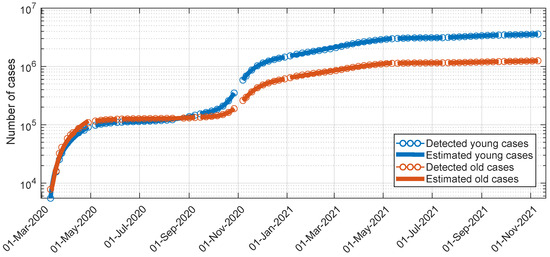
Figure 2.
Data fitting for the compartmental model: actual and estimated cumulative profiles for young subjects infected and old subjects infected (logarithmic scale).
The parameters estimated in the different scenarios () , are reported in Table 1, along with the new ones estimated in the new three scenarios G, H, and I. The same happens for the estimated initial conditions , , , that appear in Table 2. Note that, since the optimization procedure is global and since we have left the susceptible in each scenario free to change in order to consider reinfection and immunity due to vaccination, the obtained parameters differ slightly from the one reported in [23]. Even though such differences do not impact any of the considerations in [23], according to the data reported in Table 1 (values in red):

Table 1.
Estimated parameters , , in the different scenarios [ for intra-juvenile virulence; for juvenile–elder virulence; for elder–juvenile virulence; for intra-elder virulence; as average time for disease identification in young subjects; and as average time for disease identification in old subjects]. Parameter values that significantly differ from the one reported in [23] are reported in red. The new scenarios G–I are highlighted with a gray background.
Table 2.
Estimated initial conditions , , , in the different scenarios [ for the initial young subjects infected; for the initial old subjects infected; for the initial young subjects susceptible; and for the initial old subjects susceptible]. The new scenarios G–I are highlighted with a gray background.
- The juvenile–elder virulence—when compared with [23]—will appear to be smaller in scenarios c (namely, low-feedback social distancing and contact reduction intervention) and e (namely, decreased social contacts in schools at a national level and social distancing measures put in place or relaxed independently by each region) to identify successfully, within c and e, a sort of decoupling (that is lost in all the other scenarios) between the two age classes and recognize the benefits, within e, of a reduction in the social contacts in schools at a national level.
- The reasonable punctual reduction—when compared with [23]—of the intra-elder virulence during the summer of scenario c (now of the same magnitude as the intra-juvenile virulence) will preserve the already established trend of such a parameter over the scenarios.
- The increase—when compared with [23]—of the average time for disease identification in old subjects within scenario c better shapes the behavior of such a parameter by consistently moving to scenario d (re-activation of social contacts in workplaces and schools) the moment in which the elderly paid a higher level of attention to symptoms while preserving the remaining, already established trend over the scenarios.
Once the estimates of the model parameters have been obtained (Table 1 and Table 2), the values of the reproduction number, , associated with model (1) in each scenario i [m stands for model-based computation], as the average number of new infections caused by an infected person, can be computed through the formula
where denotes the biggest among the moduli of the eigenvalues of the matrix argument. The resulting mean reproduction numbers, , over read: , , , , 1, 1, , 1, 1. They are compatible with the maximum likelihood values of the national reproduction number in Figure 3, computed from raw data through the EpiEstim toolbox. This shows that model (1) is able to catch the main epidemic features along the considered scenarios.
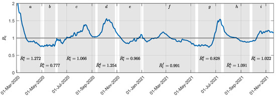
Figure 3.
National reproduction number, , within the considered time windows. Each shaded portion of the plane corresponds to a specific scenario. The mean value, (among the values corresponding to our sampling) within each time window, , is reported at the bottom of each shaded region.
5. Discussion
The following comments are reported. They provide a deep interpretation of the estimation results in Table 1, Table 2 and Table 3.
- All the estimates corresponding to the different scenarios, including the estimated , (initial young subjects infected; initial old subjects infected), allow the estimated profile to reproduce the actual one along the different scenarios satisfactorily, as shown in Figure 2.
- The number of susceptible individuals in both age groups continuously decreases in all the scenarios starting from scenario G (including additional scenario J), as an effect of the vaccination campaign starting within scenario f and continuing within G. However, a non-drastic reduction in such a number seems to confirm that the vaccination action principally protects against severe symptomatology rather than giving total immunity [24].
- Starting from scenario G, again as an effect of the vaccination campaign starting within scenario f and continuing within G, the juvenile–elder and the intra-elder virulences exhibited a large reduction. The major strength of the vaccination action for the elderly, however, allows for relatively large elder–juvenile virulence values.
- The average time for disease identification in young subjects in all the scenarios, a–f and G–I, ranges from 1 to 9 days across the scenarios. Notably, scenarios b–c have an average time of approximately 5–7 days, whereas new scenario G has a slightly longer time of about 8 days. This variation can be attributed to the fact that, after the lockdown period and related concerns, young individuals tended to pay less attention to their symptoms, particularly in scenarios b and c (covering the summer period, from 7 May 2020 to 8 September 2020). The same phenomenon was observed in new scenario G, which occurred from 19 May 2021 to 14 July 2021. This period coincided with weakened, intermittent regional actions and the second vaccination stage (booster), along with no festivities, like Christmas and Easter. In contrast, scenarios H–I exhibited a substantial reduction in the average time for disease identification among young subjects, possibly due to more immediate reliance on testing in the presence of: (i) typical entertainment habits during the summer that saw a large increase in travel (compared with previous analogous scenario c); (ii) normal reopening of schools and entertainment activities such as discos and ballrooms. These scenarios also witnessed an increase in intra-juvenile virulence (, ) compared with G ().
- Even the average time for disease identification in old subjects in all the scenarios, a–f and G–I, varies from 1 to 9 days, with less than 4 days occurring in scenarios d–f (in which the elderly paid a higher level of attention to symptoms) and H–I (corresponding to an increase of the intra-juvenile and elder–juvenile virulences).
- The elder–juvenile virulences exhibit a specific increasing trend starting from scenario e (namely, coordinated intermittent regional action), except for scenario G (namely, weakened intermittent regional actions, second vaccination stage (booster), and, mainly, no festivities, like Christmas and Easter), in which all the virulences show a relatively large reduction. The subsequent increase of intra-juvenile and elder–juvenile virulences seems to suggest a sort of greater decoupling of social habits between young subjects and old ones, and allows us to pose a question while recognizing scenario G as the most favourable one in terms of virulence values: what would have happened if, after the first vaccination campaign, the super-attenuated coordinated intermittent regional actions and the last step towards normality had been delayed until after the summer vacations, and actions like the ones in a–b, e had been performed to reduce the intra-juvenile virulence?
6. One and Two Years Later
Furthermore, new real data about the pandemic on the following time window:
- (J)
- from 1 March 2023 to 3 May 2023
Are also taken in order to allow for a direct comparison with analogous scenario a two years before and with f two years before. The estimated parameters for additional scenario J (estimated by minimizing ) appear in Table 3.
Table 3.
Estimated parameters for time window J (to be compared with a and f).
Table 3.
Estimated parameters for time window J (to be compared with a and f).
| Time Window J from 1 March 2023 to 3 May 2023 | |||||
|---|---|---|---|---|---|
From 1 March 2023 to 3 May 2023: two years later than a, one year later than f. The average time for disease identification in young subjects is larger than a and f (about 7 days compared with the previous 2–4 days). The disease has become endemic with no more strong restrictions in social habits: (i) young subjects somehow pay less attention than old ones, for whom the average time changed from 2–3 days to just 5; (ii) by forming a completely novel picture, a balance between (not small) juvenile–elder and elder–juvenile virulences appears, as never happened before, with the intra-juvenile and intra-elder virulences concurrently decreasing, when compared with f, but again being non-small, again confirming that the vaccination action has definitely attenuated severe symptomatology rather than providing total immunity. Finally, the estimate of the average reproduction number in this scenario is 1.04, again confirming the endemic nature of COVID-19 in Italy.
7. Conclusions
The epidemiological model for COVID-19 developed in [23], which considers the epidemic within the younger age group and older age group separately, has been used to provide an updated insight into the different evolution of the epidemic in the considered two age groups, while simultaneously evaluating, through the estimation of crucial model parameters, the impact of changes in social distancing measures and vaccination actions. The exact structure of the contact patterns in the general population is, in fact, still unknown to a large extent and deserves specific research efforts, to characterize better the effects of political choices that, over time, change the rules governing social distancing and behaviors.
The methodological contribution of this paper, compared with what was proposed in [23], is incremental: given the high probability of reinfection and to take into account the low probability of immunity to infection acquired by vaccination, we introduced the number of susceptible at the beginning of each time window within the set of parameters to be estimated. Such a number was fixed to the number of non-infected individuals in [23]. Interestingly and retrospectively, we have shown that the introduction of this degree of freedom did not significantly affect the results of the already analyzed scenarios a-f (in line with the results presented in [23]), showing the correctness of the hypotheses put forward in [23], as well as the robustness of the procedure. Furthermore, the new results provide a meaningful picture of the evolution of the social behaviors and the goodness of the performed strategic interventions.
The significance of this work thus lies in the application and validation of methodological frameworks proposed in [23] to newly updated data. By adopting the approach outlined in previous work, we showcase the enduring relevance of established methodologies in the ever-evolving landscape of the current pandemic. This underscores a critical message: the wealth of knowledge amassed through extensive scientific endeavors in recent years remains indispensable. As we navigate the dynamic challenges posed by COVID-19, it is imperative for policymakers and researchers alike to continuously leverage and update the methodological foundations already established. The findings of this study reinforce the notion that the synergy between established methodologies and real-time data analysis is paramount for informed decision-making. Through this, we advocate for an ongoing commitment to evidence-based practices, ensuring that our scientific insights persistently inform strategies and policies, ultimately contributing to the effective management of the res publica.
This paper underscores the significance of the extensive scientific endeavors conducted in recent years, emphasizing that the wealth of knowledge acquired must be consistently employed to interpret the ongoing situation. Serving as the conclusion to the Special Issue “New Challenges in Mathematical Modelling and Control of COVID-19 Epidemics: Analysis of Non-pharmaceutical Actions and Vaccination Strategies” we curated, it highlights the significance of the Special Issue itself, showing the importance of utilizing methodological achievements to navigate the current landscape effectively. By demonstrating how the overarching principles guide the interpretation of data, in our view, this paper further underscores the critical role that accumulated scientific insights play in addressing the complexities of the COVID-19 pandemic (as well as other pandemics) nowadays.
Future research efforts shall be devoted to analyze different model structures comparatively, even within the stochastic framework.
Author Contributions
Conceptualization: C.M.V. and F.D.R.; methodology: C.M.V. and F.D.R.; software and resources: F.D.R.; formal analysis: C.M.V. and F.D.R.; validation, investigation: C.M.V. and F.D.R.; writing—original draft: C.M.V.; writing—review and editing: C.M.V. and F.D.R. All authors have read and agreed to the published version of the manuscript.
Funding
This research received no external funding.
Data Availability Statement
The publicly archived datasets that were analyzed during the study are explicitly quoted in the paper.
Acknowledgments
The authors are grateful to E. Cottafava, in her quality of General Secretary of Fondazione GIMBE, Via Amendola, 2, 40121 Bologna, for her willingness to provide data concerning the profile of the Italian reproduction numbers over time.
Conflicts of Interest
The authors declare no conflict of interest.
References
- Qian, M.; Jiang, J. COVID-19 and social distancing. J. Public Health 2020, 30, 259–261. [Google Scholar] [CrossRef]
- Della Rossa, F.; Salzano, D.; Di Meglio, A.; De Lellis, F.; Coraggio, M.; Calabrese, C.; Guarino, A.; Cardona-Rivera, R.; De Lellis, P.; Liuzza, D.; et al. A network model of Italy shows that intermittent regional strategies can alleviate the COVID-19 epidemic. Nat. Commun. 2020, 11, 5106. [Google Scholar] [CrossRef]
- Kretzschmar, M.E.; Rozhnova, G.; Bootsma, M.C.; van Boven, M.; van de Wijgert, J.H.; Bonten, M.J. Impact of delays on effectiveness of contact tracing strategies for COVID-19: A modelling study. Lancet Public Health 2020, 5, e452–e459. [Google Scholar] [CrossRef] [PubMed]
- Keeling, M.J.; Hollingsworth, T.D.; Read, J.M. Efficacy of contact tracing for the containment of the 2019 novel coronavirus (COVID-19). J. Epidemiol. Community Health 2020, 74, 861–866. [Google Scholar] [CrossRef]
- Tupper, P.; Otto, S.P.; Colijn, C. Fundamental limitations of contact tracing for COVID-19. Facets 2021, 6, 1993–2001. [Google Scholar] [CrossRef]
- Italia, M.; Della Rossa, F.; Dercole, F. Model-informed health and socio-economic benefits of enhancing global equity and access to COVID-19 vaccines. Sci. Rep. 2023, 13, 21707. [Google Scholar] [CrossRef] [PubMed]
- Kucharski, A.J.; Klepac, P.; Conlan, A.J.; Kissler, S.M.; Tang, M.L.; Fry, H.; Gog, J.R.; Edmunds, W.J.; Emery, J.C.; Medley, G.; et al. Effectiveness of isolation, testing, contact tracing, and physical distancing on reducing transmission of SARS-CoV-2 in different settings: A mathematical modelling study. Lancet Infect. Dis. 2020, 20, 1151–1160. [Google Scholar] [CrossRef]
- Musa, S.S.; Qureshi, S.; Zhao, S.; Yusuf, A.; Mustapha, U.T.; He, D. Mathematical modeling of COVID-19 epidemic with effect of awareness programs. Infect. Dis. Model. 2021, 6, 448–460. [Google Scholar] [CrossRef]
- Ancona, C.; Lo Iudice, F.; Garofalo, F.; De Lellis, P. A model-based opinion dynamics approach to tackle vaccine hesitancy. Sci. Rep. 2022, 12, 11835. [Google Scholar] [CrossRef] [PubMed]
- Maji, C.; Al Basir, F.; Mukherjee, D.; Ravichandran, C.; Nisar, K. COVID-19 propagation and the usefulness of awareness-based control measures: A mathematical model with delay. AIMs Math 2022, 7, 12091–12105. [Google Scholar] [CrossRef]
- Thunström, L.; Newbold, S.C.; Finnoff, D.; Ashworth, M.; Shogren, J.F. The benefits and costs of using social distancing to flatten the curve for COVID-19. J. Benefit-Cost Anal. 2020, 11, 179–195. [Google Scholar] [CrossRef]
- Moosa, I.A. The effectiveness of social distancing in containing COVID-19. Appl. Econ. 2020, 52, 6292–6305. [Google Scholar] [CrossRef]
- Silva, P.C.; Batista, P.V.; Lima, H.S.; Alves, M.A.; Guimarães, F.G.; Silva, R.C. COVID-ABS: An agent-based model of COVID-19 epidemic to simulate health and economic effects of social distancing interventions. Chaos Solitons Fractals 2020, 139, 110088. [Google Scholar] [CrossRef]
- Childs, M.L.; Kain, M.P.; Kirk, D.; Harris, M.; Couper, L.; Nova, N.; Delwel, I.; Ritchie, J.; Mordecai, E.A. The impact of long-term non-pharmaceutical interventions on COVID-19 epidemic dynamics and control. MedRxiv 2020. [Google Scholar] [CrossRef]
- Goldsztejn, U.; Schwartzman, D.; Nehorai, A. Public policy and economic dynamics of COVID-19 spread: A mathematical modeling study. PLoS ONE 2020, 15, e0244174. [Google Scholar] [CrossRef] [PubMed]
- Childs, M.L.; Kain, M.P.; Harris, M.J.; Kirk, D.; Couper, L.; Nova, N.; Delwel, I.; Ritchie, J.; Becker, A.D.; Mordecai, E.A. The impact of long-term non-pharmaceutical interventions on COVID-19 epidemic dynamics and control: The value and limitations of early models. Proc. R. Soc. B 2021, 288, 20210811. [Google Scholar] [CrossRef] [PubMed]
- Onder, G.; Rezza, G.; Brusaferro, S. Case-fatality rate and characteristics of patients dying in relation to COVID-19 in Italy. Jama 2020, 323, 1775–1776. [Google Scholar] [CrossRef] [PubMed]
- Ruan, Q.; Yang, K.; Wang, W.; Jiang, L.; Song, J. Clinical predictors of mortality due to COVID-19 based on an analysis of data of 150 patients from Wuhan, China. Intensive Care Med. 2020, 46, 846–848. [Google Scholar] [CrossRef] [PubMed]
- Zou, Y.; Yang, W.; Lai, J.; Hou, J.; Lin, W. Vaccination and quarantine effect on COVID-19 transmission dynamics incorporating Chinese-spring-festival travel rush: Modeling and simulations. Bull. Math. Biol. 2022, 84, 30. [Google Scholar] [CrossRef] [PubMed]
- Guo, Y.; Liu, X.; Deng, M.; Liu, P.; Li, F.; Xie, N.; Pang, Y.; Zhang, X.; Luo, W.; Peng, Y.; et al. Epidemiology of COVID-19 in older persons, Wuhan, China. Age Ageing 2020, 49, 706–712. [Google Scholar] [CrossRef]
- Balabdaoui, F.; Mohr, D. Age-stratified discrete compartment model of the COVID-19 epidemic with application to Switzerland. Sci. Rep. 2020, 10, 21306. [Google Scholar] [CrossRef] [PubMed]
- Bentout, S.; Tridane, A.; Djilali, S.; Touaoula, T.M. Age-structured modeling of COVID-19 epidemic in the USA, UAE and Algeria. Alex. Eng. J. 2021, 60, 401–411. [Google Scholar] [CrossRef]
- Verrelli, C.M.; Della Rossa, F. Two-age-structured COVID-19 epidemic model: Estimation of virulence parameters to interpret effects of national and regional feedback interventions and vaccination. Mathematics 2021, 9, 2414. [Google Scholar] [CrossRef]
- Mohammed, I.; Nauman, A.; Paul, P.; Ganesan, S.; Chen, K.H.; Jalil, S.M.S.; Jaouni, S.H.; Kawas, H.; Khan, W.A.; Vattoth, A.L.; et al. The efficacy and effectiveness of the COVID-19 vaccines in reducing infection, severity, hospitalization, and mortality: A systematic review. Hum. Vaccines Immunother. 2022, 18, 2027160. [Google Scholar] [CrossRef]
Disclaimer/Publisher’s Note: The statements, opinions and data contained in all publications are solely those of the individual author(s) and contributor(s) and not of MDPI and/or the editor(s). MDPI and/or the editor(s) disclaim responsibility for any injury to people or property resulting from any ideas, methods, instructions or products referred to in the content. |
© 2024 by the authors. Licensee MDPI, Basel, Switzerland. This article is an open access article distributed under the terms and conditions of the Creative Commons Attribution (CC BY) license (https://creativecommons.org/licenses/by/4.0/).