Article

Transfer Learning with ResNet3D-101 for Global Prediction of High Aerosol Concentrations

by
Dušan P. Nikezić
*,
Dušan S. Radivojević
,
Ivan M. Lazović
,
Nikola S. Mirkov
and
Zoran J. Marković
Vinča Institute of Nuclear Sciences, National Institute of the Republic of Serbia, University of Belgrade, 11000 Belgrade, Serbia
*
Author to whom correspondence should be addressed.
Mathematics 2024, 12(6), 826; https://doi.org/10.3390/math12060826
Submission received: 20 February 2024 / Revised: 1 March 2024 / Accepted: 8 March 2024 / Published: 12 March 2024
(This article belongs to the Special Issue Advanced Research in Image Processing and Optimization Methods)

Abstract

:
In order to better predict the high aerosol concentrations associated with air pollution and climate change, a machine learning model was developed using transfer learning and the segmentation process of global satellite images. The main concept of transfer learning lies on convolutional neural networks and works by initializing the already trained model weights to better adapt the weights when the network is trained on a different dataset. The transfer learning technique was tested with the ResNet3D-101 model pre-trained from a 2D ImageNet dataset. This model has performed well for contrail detection to assess climate impact. Aerosol distributions can be monitored via satellite remote sensing. Satellites can monitor some aerosol optical properties like aerosol optical thickness. Aerosol optical thickness snapshots were the input dataset for the model and were obtained from NASA’s Terra-Modis satellite; the output images were segmented by comparing the pixel values with a threshold value of 0.8 for aerosol optical thickness. Hyperparameter optimization finds a tuple of hyperparameters that yields an optimal model that minimizes a predefined loss function on given independent data. The model structure was adjusted in order to improve the performance of the model by applying methods and hyperparameter optimization techniques such as grid search, batch size, threshold, and input length. According to the criteria defined by the authors, the distance domain criterion and time domain criterion, the developed model is capable of generating adequate data and finding patterns in the time domain. As observed from the comparison of relative coefficients for the criteria metrics proposed by the authors, ddc and dtc, the deep learning model based on ConvLSTM layers developed in our previous studies has better performance than the model developed in this study with transfer learning.

1. Introduction

Deep neural networks are mathematical structures that are very hardware-demanding in training, especially in the big data and computer vision domain. The solution lies in re-using the model weights from the pre-trained models for computer vision data [1]. In most new research, transfer learning is used, where only the last layer can be changed with new data in an already trained neural network. Training a new network sometimes requires several days, or even weeks, depending on the complexity of the problem and the amount of training data, so the use of transfer learning reduces the learning time. Transfer learning uses the knowledge gained from the previous task in order to produce efficient results for similar tasks. Transfer learning is most commonly used in image classification, image prediction, and natural language processing. There are a lot of pre-trained models with pre-trained weights available from Keras for images.
Transfer learning does not change the weights in layers to be re-initialized, so layers do not change during training. Newly added layers must be trained on the input dataset in order for the developed model to make predictions. Optionally, the performance of the new model can be improved by fine tuning it at a very low learning rate. This will increase the model’s performance on the new data and prevent overfitting. In this research, several structures of the ResNet3D-101 model were tested with other versions of this model for transfer learning. In addition to the mentioned classic techniques of transfer learning and fine tuning, we tried using the model structure without trained weights on the ImageNet dataset, as well as the specified weights as an initial state without freezing the weights during training. This research showed that the ResNet3D-101 model trained on the ImageNet 2D dataset with unfrozen weights of layers performed the best during training.
Transfer learning is usually used with convolutional neural networks for classification. Low-level features, i.e., lines, are extracted from convolutional layers closer to the input, while middle layers catch complex abstract features from the lower-level features extracted. Classification is performed with layers closer to the output. The use of transfer learning for recurrent neural networks such as LSTM is not common. LSTM cells are recurrent, take input embedded vectors, pass hidden states, and output a prediction vector. It is not useful to transfer the weights of the LSTM cells to train the output layer. The output layer serves for non-linearity with a softmax function for final classification. Transfer learning in an LSTM can be used with an associated embedding layer to speed up training and improve accuracy. The reason for this is that convolutional neural networks have similar input images, while LSTMs usually have different input sequences.
This work is the continuation of the research conducted in two previous studies [2,3] with the same goal, i.e., to use measurements from the Moderate Resolution Imaging Spectroradiometer (MODIS) by NASA satellite Terra, in order to forecast global aerosol concentrations through deep learning. Furthermore, transfer learning was implemented in this study in order to develop a model for predicting global high concentrations of aerosol optical thickness (AOT). These images were produced using the SDS AOD_550_Dark_Target_Deep_Blue_Combined, which has a wavelength reference of 550 nm, as reported by satellite data products. The NASA Earth Observations website explains that the aerosol data product algorithms take advantage of MODIS’ wide spectral range and high spatial resolution with daily global coverage. These unique MODIS characteristics allow excellent cloud rejection while maintaining the high statistics of cloud-free pixels. MODIS data are available through LANCE generally within 60 to 125 min after a satellite observation. The disadvantages include their limited spatial resolution and reliance on specific spectral channels.
As concentrations of global aerosol increase in frequency and intensity, it has become increasingly important to improve monitoring, prediction, and early warning systems in order to help decision support systems. Therefore, the aim of this study is to develop a model with a prediction of the peak AOT index for early warning. The AOT is more accurate over water surfaces than over land surfaces. In most cases, the AOT is smaller than 0.4; an AOT > 0.6 occurs only 2% of the time and an AOT > 0.4 occurs only 6% of the time [4]. The threshold value for high AOT concentrations used in this study was chosen to be above 0.8, and through that the developed model forecasts an AOT in the range of (0.8, 1] for the eighth day [5].

Literature Review and Related Work

There are many top-performing pre-trained models in Keras that can be used as the backbone for a new model in computer vision and image processing problems [6]. One of the many performing well in Top-1 and Top-5 error rates on ImageNet is the baseline model residual neural network (ResNet) with different versions, particularly version ResNet-101, which is a 101-layer deep convolutional neural network. ResNet resolves the problem of vanishing gradients, and thus supports up to thousands of convolutional layers. The weight layers of ResNet acquire residual functions with references to the layer inputs [7]. ResNet-101, which consists of residual blocks, showed better results than VGG-16 did in [7]. Moreover, the updates to modern training methods and the improved scaling strategy have led to the remarkable endurance of ResNet architecture to be achieved significantly faster than that of EfficientNets [8].
A main difference between videos and images is the additional temporal dimension. Combining features across spatial and temporal dimensions can be achieved using 3D convolutions or self-attention [8]. In our study [3], we implemented a self-attention mechanism in our developed model. Spatio-temporal 3D kernels in convolutional networks learn spatiotemporal features from videos in order to recognize actions. Three-dimensional ResNets performing 3D convolution and 3D pooling have shown good performance without overfitting despite the large number of parameters of the model [9]. Furthermore, various ResNets like ResNet-101 showed progress in image captioning, object detection, and semantic segmentation [10]. Three-dimensional ResNets could be used for human pose estimation based on self-supervision and to retrace the history of 2D CNNs and ImageNet [11,12]. Transfer learning using ResNet3D-101 has given good results in many areas such as on kinetics datasets or for the classification of industrial parts [13].
The main concept of how to incorporate temporal contexts into image sequences was presented in a study [14] for the Kaggle competition “Google Research-Identify Contrails to Reduce Global Warming”. The researchers employed promising image segmentation techniques including using the ResNet backbone [14]. Inflating the 2D convolutional neural network into 3D is the current approach used for video classification. It converts 2D classification models into 3D by training multiple frames at once instead of one by, one and the obtained results show that the multi-frame model is better than the single-frame based models. This proves that the multi-frame model is able to use temporal contexts to improve accuracy [14]. Furthermore, ResNet3D-101 showed the best result through the evaluation metric per-pixel performance using the area under the precision recall curve (AUC-PR) among the other ResNet models like ResNet-101 [14].
Study [15] was also used for this research with the main idea being to split 3D MRI scans into 2D image slices. By carrying this out, classification can be applied on image slices independently, benefitting from the concept of transfer learning [15]. The ResNet3D-101 transfer learning model, which was pre-trained with 2D images, was used in this study, and ResNet3D-101 was downloaded from GitHub [16].

2. Data and Methodology

Pre-Training Process

Satellite image time series are sequences of satellite images that record a given area at consecutive moments. Since the input dataset comprises continuous snapshots of AOT as a sequence every 8 days, the aims of this study were to develop a model that is capable of learning patterns and relationships and of extracting features from time series of satellite images in order to predict the AOT for the next 8 days [2]. The input dataset consists of snapshots from 18 February 2000 to 17 November 2023 taken every 8 days with a total of 1094 images [17]. In the present study, satellite-retrieved AOT was used as a dataset, MODAL2_E_AER_OD. The input data were sequences of 10 Terra MODIS images in RGB format resized to 400 × 200 pixels. The input data format was 3D since 10 images in one sequence make up the third temporal component, and the output was one 2D segmented image with the same resolution, 200 × 400. The original input dataset was converted into 2 values in images, black/white (0/1), for binary image segmentation. The model was trained for classifying each pixel in output segmented images. Values represented by 0 are unread data and AOT values less than 0.8 (black pixels [0, 0.8]), while values represented by 1 are AOT values above 0.8 (white pixels (0.8, 1]). Image segmentation shows probabilities from 0 to 1, encoded as bytes ranging from 0 to 255 [18]. The input dataset was split into train, validation, and test subsets, so the train set was 70%, the validation set was 10% and the test set was 20% to evaluate the model.
The output images, like the pre-processed input images, are segmented, which implies the existence of only two sets of affiliations. The model outputs a result between 0 and 1 for each pixel, indicating the level of confidence that the pixel has a high AOT concentration. In this way, the segmentation marked places with a high concentration of AOT that can be potentially dangerous for human health and the environment. Given that the satellite images were generated in 8-day increments, our model based on the previous satellite snapshots predicts, for the eighth day, which regions will have AOT concentrations greater than 0.8.
Figure 1 shows an original snapshot of the AOT and its pre-processed segmented image.
The two evaluation criteria that defined are as follows [19]:
  • The distance domain criterion (ddc) (the machine learning (ML) model is capable of generating adequate data if metrics for the predicted data, in comparison with the original data, are equal or better than an average difference between randomly selected output data from the database).
The ddc criterion is calculated as follows:
d d c = d r 1 , r 2
where r1 and r2 are two random elements from the original output dataset, d represents distance metrics, and < > denotes an averaging operator.
  • The time domain criterion (dtc) (the ML model is capable of finding patterns in the time domain if metrics for predicted data, in comparison with the original data, are equal or better than an average difference of two adjacent output data from the database).
The dtc criterion is calculated as follows:
d t c = d y n , y n + 1
where yn and yn+1 are two consecutive time elements from the original output dataset, d represents distance metrics, and < > denotes an averaging operator.
These two criteria were used to evaluate the segmented dataset before training the model, and the results are shown in Table 1. The metrics that were used when calculating the criteria were root mean square error (RMSE), accuracy (ACC), F1 score (F1), Jaccard score (JS), and area under curve for precision vs. recall (AUC-PR).
Although the RMSE metric is commonly used for regression, there are cases when it is justifiable to use this metric for classification as well. When classes are defined not as separate objects, but as different intensities or concentrations of the same physical quantity as in our research, MSE and RMSE metrics are convenient to use [19,20,21].
The model fully meets the criteria if all metrics on the test set are better or equal to the values listed in Table 1. The model partially meets the criteria if some test set metrics are better or equal to the values listed in Table 1. The model fails the criteria if all test set metrics are worse than those listed in Table 1.

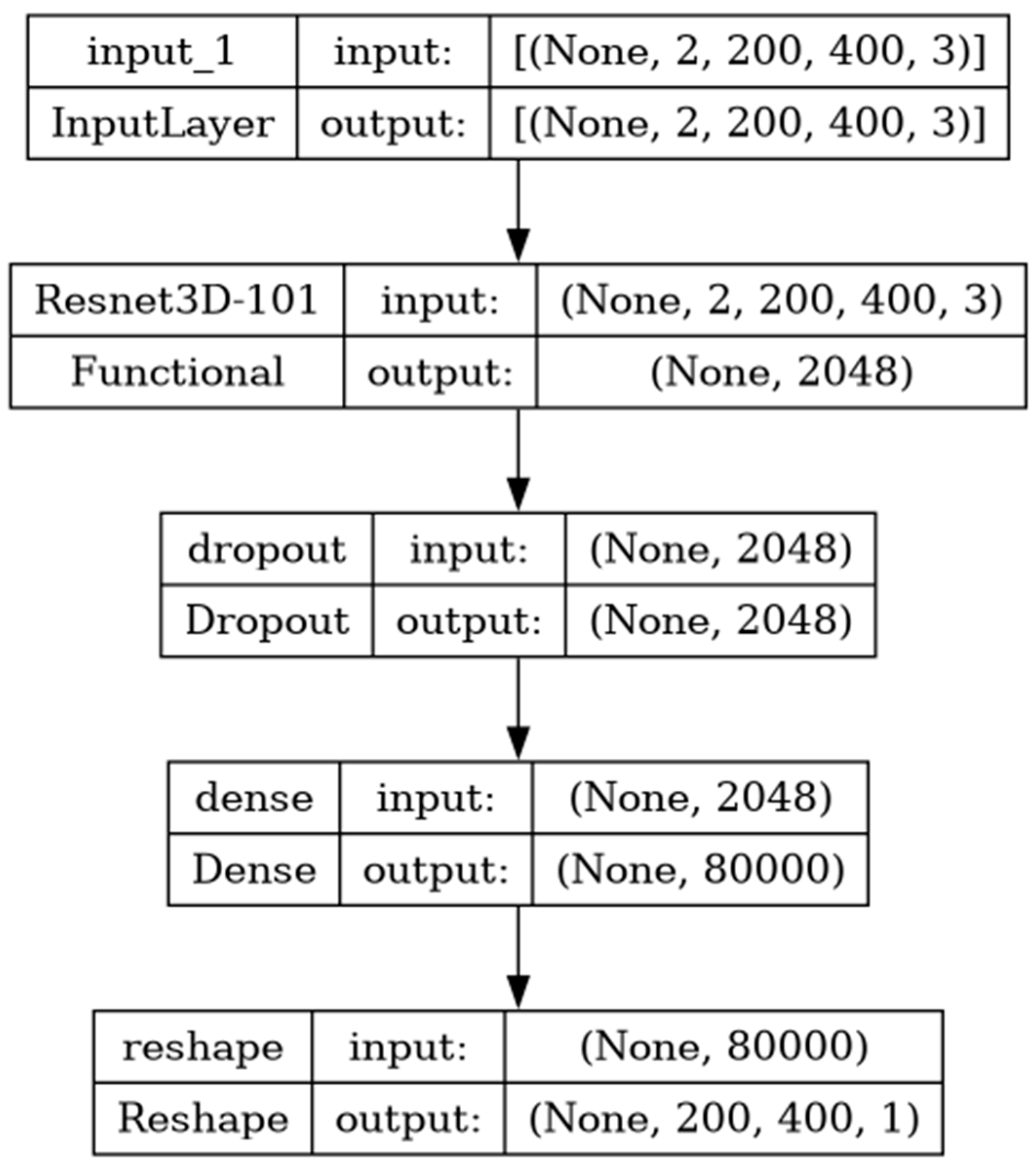
3. Transfer Learning Model

The residual network (ResNet) is a deep learning model intended for computer vision tasks, and it is characterized by the fact that it enables the use of a huge number of convolutional layers using the skip connections technique. Skipping some layers results in residual blocks that are partly connected to the nearest layers and partly connected to distant layers. This technique solves the vanishing and exploding gradient problem caused by the many layers connected in a deep neural network.
Given that the problem of predicting high concentrations of aerosols represents a spatial–temporal problem, we decided to use three-dimensional processing with the help of the ResNet model. The transfer learning technique is used most often in situations where the dataset for model training is small. This adds to knowledge already acquired from another task, thus compensating for the current small data set.
As a goal of this study, transfer learning was implemented with the ResNet3D-101 model, which was pre-trained on the ImageNet dataset, followed by Dropout layer and Dense layer for the output classification task, as shown in Figure 2.
The model shown in Figure 2 depicts the basic structure to which further improvements were made. The pre-trained ResNet3D-101 model with a defined pooling output layer performs feature extraction from 3D input data. In order to prevent overfitting during training, a dropout layer was added. Given that the total number of pixels in the output segmented image was 80,000, the same number of neurons were used in the next Dense layer. Since the output image has dimensions of 200 × 400 pixels, a reshape layer was added at the end, which converted a 1D vector into a 2D image according to the segmented output. In this way, each neuron from the Dense layer represents one output pixel of the segmented AOT image.
After the model structure was adapted for transfer learning as described, the hyperparameters for tuning were defined. The impact of the sequential length of the input data and that of the optimal threshold value of classification were examined.
The required parameters based on the previously defined model are the type of pooling output layer of the ResNet3D-101 model, dropout value, activation function of the Dense layer, optimizer of the training process, weight samples during training, batch size, threshold value, and optimal number of input images for prediction. The initial learning rate was set to 0.00005, and in the learning process it was reduced via the ReduceLROnPlateau method with an order of magnitude with patience = 2 and with a monitor for the binary accuracy of the validation set. The EarlyStopping method was also used, where the monitor was set to the loss of the validation set and patience = 6. These two regulation methods, in addition to the Dropout layer, serve to prevent overfitting.
In order to obtain the best model prediction results, the technique of initializing weights in the train set was tried. Target output images were set based on the number of class occurrences of 0 and 1 whose weights were determined using the compute_class_weight method from the Scikit-learn library. The range of values obtained based on the above was from 0.53 to 1.41, which is a relatively narrow range for weights, so the power of these values was also used in the parameter search. During training, BinaryCrossentropy was used as the loss function, and the metric was BinaryAccuracy.

4. Results and Discussion

4.1. Grid Search

In the first part of hyperparameter tuning, a grid search of the following parameters was performed: the power of sample weights from the train set (0, 3, 5), type of pooling layer for ResNet3D-101 model (max; avg), dropout value (0.1, 0.2, 0.3), activation function of the Dense layer (sigmoid; hard_sigmoid], and optimizer (Adam, Nadam and AdamW). The metric used for this process was AUC-PR. The best obtained combination of parameters was in the order 0, max, 0.3, sigmoid, Nadam with an achieved AUC-PR score of 0.4980, as shown in Table S1 (Supplementary Materials).

4.2. Effect of Batch Size

During the previous test, the batch size was set to 32, which had a favorable effect on the total training time. Therefore, the influence of batch size with previously defined values of hyperparameters was additionally checked. Table 2 shows that the best batch size value is 4 with an AUC-PR value of 0.50189.

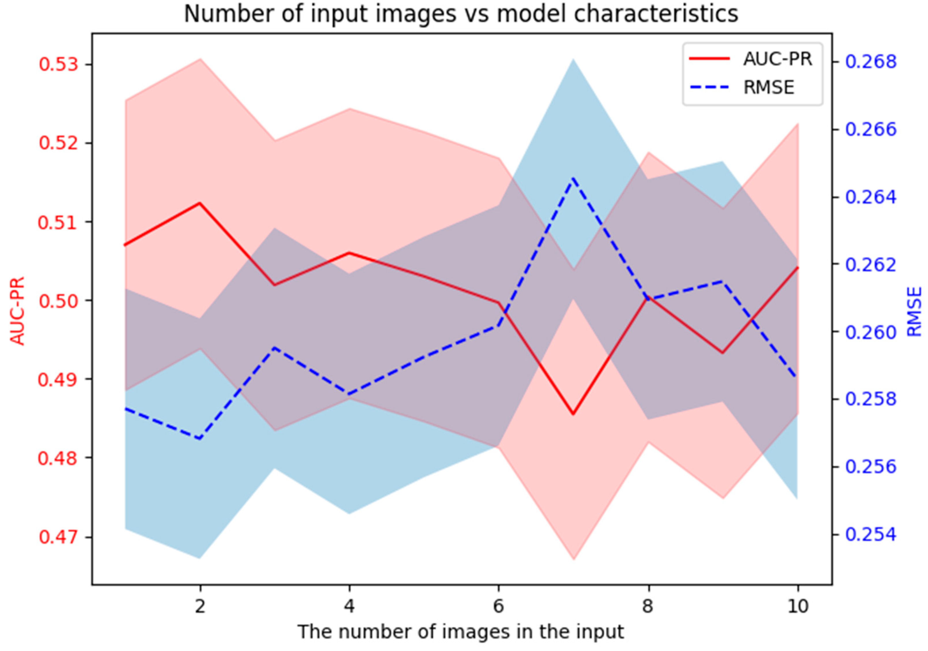
4.3. Influence of Input Length

The performance of the model can be improved by using multiple input frames across the temporal context. Detection with different numbers of input frames was carried out in study [14]. Therefore, input frames from 1 to 10 of the timestep of eight days were used to test model performance, and the obtained results are shown in Figure 3.
The examination of the influence of the input number of images on the characteristics of the model was performed with 10 repetitions and with the model structure and the parameters previously defined. In Figure 3, the mean values of the AUC-PR and RMSE metrics are shown by lines, while the shaded areas represent the uncertainty calculated as double the standard deviation of the obtained results per example. It can be concluded that the optimal number of input images is two, with the best obtained results being 0.5123 and 0.2568 for AUC-PR and RMSE, respectively.

4.4. Classification Threshold

In order to improve the achieved results of the model, one additional method in the field of classification is finding the optimal value for the threshold. The default value of this parameter is 0.5, so all values greater than it are classified as 1, and all values less than it are classified as 0. The default value is not always the best solution, so the practice is to find a better value.
Searching for the optimal candidate for threshold value was achieved with the receiver operating characteristic (ROC) method, which suggests good candidates based on predicted and actual values. For each proposed value, a pair comprising the true positive rate TPR and false positive rate FPR was obtained. The threshold candidate was found to be the maximum value of the difference between TPR and FPR, and it was determined to be a value of 0.063.
Applying the new threshold value resulted in an increase in the AUC-PR metric of 10.2%, but all other applied metrics significantly worsened. Based on the comparison of the metrics, it was found that the default value of 0.5 favors the RMSE and ACC metrics over the other metrics, and the value of 0.063 favors the AUC-PR metric over the other metrics. The optimal solution was found in the search for values between the two previously mentioned. A manual search determined that a threshold value of 0.38 gives balanced and better results for the metrics used, and this threshold value was used in further work.

4.5. Obtained Results

Based on all previously defined parameters, the final training of the model was performed. The model learning process during training is shown in Figure 4.
Figure 4 depicts that the applied regulation methods resulted in the absence of overfitting and that the metrics are slowly approaching the best values through the epochs. After the training process, model prediction was performed on the test subset, and the obtained results are given in Table 3.
It can be concluded from Table 3 that the metrics for the validation set are better than the metrics for the test set, and that also the metrics for the training set are better than the metrics for the validation set and test set. Given that model training relies mostly on the train set, and due to the regulatory methods on the validation set, the obtained results were expected. Therefore, the metrics for the test set can be considered objective and will be used in the further analyses.
In the process of model optimization, several methods were used, such as grid search, batch size, the influence of the length of the input sequence, and a search for the threshold value of the classification. The entire tuning process led to an increase in the AUC-PR from the mean value of the results achieved during the grid search of 0.4319 to the final value after tuning of 0.5532. The share of benefits of the mentioned methods in the overall improvement is as follows: batch size, input sequence length, threshold value search, and grid search, which are 3%, 9%, 33%, and 55%, respectively.
Given that the obtained results of the model prediction depend to a great extent on the database itself and the method used for its preparation, an objective way to discuss this topic is to discuss it only if the obtained results are compared with the above-mentioned criteria. By comparing the values of the model’s metrics from the test set with the values from Table 1, it can be concluded, based on the mentioned criteria, that the model can generate adequate data, and recognize patterns in the time domain. In order to better compare the results among different authors and their works, taking into account different databases and different preparation methods, favoring certain metrics according to the threshold and in accordance with other techniques, we suggest introducing the relative coefficient of the metric dr, as shown in Equations (3) and (4):
d d r = d m d d c
where ddr is the metric relative coefficient for the distance domain criterion, dm is the model prediction metric for the test set, and ddc is the distance domain criterion metric.
d t r = d m d t c
where dtr is the metric relative coefficient for the time domain criterion, dm is the model prediction metric for the test set, and dtc is the time domain criterion metric.
Regarding the use of the mentioned coefficients, the metric relative coefficient for the distance domain criterion, ddr, can be used to compare any two ML models, while the metric relative coefficient for the time domain criterion, dtr, is suitable only for the prediction of time-dependent quantities, as in sequences. Based on Equations (3) and (4), it is obvious that the mentioned coefficients have a similar nature to that of the metrics they are used for, in the sense that if the metric is better when it is smaller, then this coefficient is also better when it is smaller and vice versa.
The fact that we defined the classes according to the intensity of the AOT value, as we mentioned above, gives us the opportunity to make a qualitative comparison of this work with our previous works [2,3] with the help of the RMSE metric and, to define relative coefficients, with the help of Equations (3) and (4). The relative coefficients of the metrics based on the defined criteria are shown in Table 4.
As can be seen from Table 4, the proposed relative coefficients of the RMSE metric have high sensitivity, which is why they are suitable for comparing different ML models. The model that most reliably generates data from the above is ConvLSTM-SA, which is based on ConvLSTM layers with an added self-attention layer [3] with a ddr coefficient for the RMSE metric of 0.6584, while the model that best follows the changes in the time domain is the ConvLSTM model proposed in [2] with an achieved dtr coefficient for the RMSE metric of 0.7582.
The advantage of the ConvLSTM model compared with the other models is reflected in the better finding of patterns in the time domain, and disadvantage is the prediction of satellite AOT images that contain some undefined pixels. The advantage of the ConvLSTM-SA model is better image reproduction than that of the other two models, and its disadvantage is the weaker detection of changes in the time domain than that of the model without the self-attention layer. The advantage of the ResNet3D-101 model compared with the other two models is that its predictions are much easier to interpret because the pixels are segmented and focus only on high-concentration aerosols, while the disadvantage of it is its weaker characteristics according to the relative ddr and dtr coefficients.

5. Conclusions and Future Research

Using a machine learning method to predict high concentrations of aerosols in the air provides an additional modern approach to solving this global problem. It is a known fact that high concentrations of aerosols are mainly associated with air pollution, that is, with poor air quality, which can have a negative impact on human health [22]. Predictions of high aerosol concentrations at specific locations can be useful for people to plan activities with increased health risks, as well as long-term ecological plans. Compared to previous models, the model from this work provides information for large concentrations of AOT that are expected in the following period at specific locations represented by pixels.
In order to forecast high concentrations of AOT on a global level, we adapted and optimized the pre-trained model ResNet3D-101. The idea for this study was developed based on a scientific paper with a similar concept from Google Research where the ResNet3D-101 model was favored as the best for remote satellite images. Transfer learning with the ResNet3D-101 model was performed with initial weights obtained from the ImageNet model, and the weights were unfrozen throughout the training. Based on the distance and time domain criteria that were proposed by the authors, the developed model is capable of generating adequate data and finding patterns in the time domain.
By comparing this model with models from our previous studies using the relative coefficients ddr and dtr for RMSE metrics that were proposed by the authors, it was shown that models with ConvLSTM layers produce less errors than the model developed in this study does and should be used as a direction for future research.

Supplementary Materials

The following supporting information can be downloaded at https://www.mdpi.com/article/10.3390/math12060826/s1, Table S1: Grid search.

Author Contributions

Conceptualization, D.P.N. and I.M.L.; methodology, D.S.R. and N.S.M.; formal analysis, Z.J.M. and D.S.R.; investigation, D.P.N. and I.M.L.; writing—original draft preparation, D.P.N. and Z.J.M.; writing—review and editing: D.S.R. and N.S.M. All authors have read and agreed to the published version of the manuscript.

Funding

The research presented in this paper was completed with the financial support of the Ministry of Science, Technological Development and Innovation of the Republic of Serbia, with the funding of scientific research work from the University of Belgrade, Vinča Institute of Nuclear Sciences (Contract No. 451-03-66/2024-03/200017).

Data Availability Statement

No new data were created or analyzed in this study. Data sharing is not applicable to this article.

Acknowledgments

The authors gratefully acknowledge “Cloud Native d.o.o., Belgrade” for their support in providing the cloud hardware and software resources necessary for the present research. We specifically express our gratitude to Dario Ristić and Jana Petrović as experts in cloud native technology. The authors gratefully acknowledge NASA Earth Observations (NEO) for their efforts in making the data available. The authors gratefully acknowledge the support of Kaggle under Google LLC with the web-based data science environment and data science competition platform used for this research.

Conflicts of Interest

The authors declare no conflicts of interest.

References

  1. Bichri, H.; Chergui, A.; Hain, M. Image Classification with Transfer Learning Using a Custom Dataset: Comparative Study. Procedia Comput. Sci. 2023, 220, 48–54. [Google Scholar] [CrossRef]
  2. Nikezić, D.P.; Ramadani, U.R.; Radivojević, D.S.; Lazović, I.M.; Mirkov, N.S. Deep Learning Model for Global Spatio-Temporal Image Prediction. Mathematics 2022, 10, 3392. [Google Scholar] [CrossRef]
  3. Radivojević, D.S.; Lazović, I.M.; Mirkov, N.S.; Ramadani, U.R.; Nikezić, D.P. A Comparative Evaluation of Self-Attention Mechanism with ConvLSTM Model for Global Aerosol Time Series Forecasting. Mathematics 2023, 11, 1744. [Google Scholar] [CrossRef]
  4. Brennan, J.; Kaufman, Y.; Koren, I.; Li, R.R. Aerosol-Cloud Interaction-Misclassification of MODIS Clouds in Heavy Aerosol. IEEE Trans. Geosci. Remote Sens. 2005, 43, 911. [Google Scholar] [CrossRef]
  5. Aerosol Optical Thickness (AOT). Available online: https://discover.data.vic.gov.au/dataset/aerosol-optical-thickness-aot (accessed on 19 January 2024).
  6. Keras Applications. Available online: https://keras.io/api/applications/ (accessed on 27 January 2024).
  7. He, K.; Zhang, X.; Ren, S.; Sun, J. Deep residual learning for image recognition. In Proceedings of the IEEE Computer Society Conference on Computer Vision and Pattern Recognition (CVPR), Las Vegas, NV, USA, 27–30 June 2016; pp. 770–778. [Google Scholar] [CrossRef]
  8. Bello, I.; Fedus, W.; Du, X.; Cubuk, E.D.; Srinivas, A.; Lin, T.Y.; Shlens, J.; Zoph, B. Revisiting ResNets: Improved Training and Scaling Strategies. Adv. Neural Inf. Process. Syst. 2021, 34, 22614–22627. [Google Scholar] [CrossRef]
  9. Du, X.; Li, Y.; Cui, Y.; Qian, R.; Li, J.; Bello, I. Revisiting 3D ResNets for Video Recognition. arXiv 2021, arXiv:2109.01696. [Google Scholar]
  10. Hara, K.; Kataoka, H.; Satoh, Y. Learning Spatio-Temporal Features with 3D Residual Networks for Action Recognition. In Proceedings of the 2017 IEEE International Conference on Computer Vision Workshop (ICCVW), Venice, Italy, 22–29 October 2017; pp. 3154–3160. [Google Scholar]
  11. Bao, W.; Ma, Z.; Liang, D.; Yang, X.; Niu, T. Pose ResNet: 3D Human Pose Estimation Based on Self-Supervision. Sensors 2023, 23, 3057. [Google Scholar] [CrossRef] [PubMed]
  12. Hara, K.; Kataoka, H.; Satoh, Y. Can Spatiotemporal 3D CNNs Retrace the History of 2D CNNs and ImageNet? In Proceedings of the 2018 IEEE/CVF Conference on Computer Vision and Pattern Recognition (CVPR), Salt Lake City, UT, USA, 18–22 June 2018; pp. 6546–6555. [Google Scholar]
  13. Merino, I.; Azpiazu, J.; Remazeilles, A.; Sierra, B. 3D Convolutional Neural Networks Initialized from Pretrained 2D Convolutional Neural Networks for Classification of Industrial Parts. Sensors 2021, 21, 1078. [Google Scholar] [CrossRef] [PubMed]
  14. Yue-Hei Ng, J.; McCloskey, K.; Cui, J.; Meijer, V.R.; Brand, E.; Sarna, A.; Goyal, N.; Van Arsdale, C.; Geraedts, S. OpenContrails: Benchmarking Contrail Detection on GOES-16 ABI. arXiv 2023, arXiv:2304.02122. [Google Scholar]
  15. Ebrahimi, A.; Luo, S.; Chiong, R. Introducing Transfer Learning to 3D ResNet-18 for Alzheimer’s Disease Detection on MRI Images. In Proceedings of the 2020 35th International Conference on Image and Vision Computing New Zealand (IVCNZ), Wellington, New Zealand, 25–27 November 2020. [Google Scholar]
  16. ZFTurbo/Classification_Models_3D. Available online: https://github.com/ZFTurbo/classification_models_3D (accessed on 27 January 2024).
  17. Index of /archive/rgb/MODAL2_E_AER_OD. Available online: https://neo.gsfc.nasa.gov/archive/rgb/MODAL2_E_AER_OD/ (accessed on 18 November 2023).
  18. Hoffman, J.P.; Rahmes, T.F.; Wimmers, A.J.; Feltz, W.F. The Application of a Convolutional Neural Network for the Detection of Contrails in Satellite Imagery. Remote Sens. 2023, 15, 2854. [Google Scholar] [CrossRef]
  19. Radivojević, D. Introducing two evaluation criteria for the next data prediction using machine learning models. In Proceedings of the DSC Europe, Belgrade, Serbia, 20–24 November 2023. [Google Scholar] [CrossRef]
  20. Beleites, C.; Salzer, R.; Sergo, V. Validation of soft classification models using partial class memberships: An extended concept of sensitivity & co. applied to grading of astrocytoma tissues. Chemom. Intell. Lab. Syst. 2013, 122, 12–22. [Google Scholar] [CrossRef]
  21. Brier, G.W. Verification of forecasts expressed in terms of probability. Mon. Weather Rev. 1950, 78, 1–3. [Google Scholar] [CrossRef]
  22. Arfin, T.; Pillai, A.M.; Mathew, N.; Tirpude, A.; Bang, R.; Mondal, P. An overview of atmospheric aerosol and their effects on human health. Environ. Sci. Pollut. Res. 2023, 30, 125347–125369. [Google Scholar] [CrossRef] [PubMed]
Figure 1. (a) Original snapshot of AOT; (b) segmented image with an AOT threshold of 0.8.
Mathematics 12 00826 g001
Figure 2. Plot of the developed model.
Mathematics 12 00826 g002
Figure 3. The obtained results for model performance depending on the number of input frames.
Mathematics 12 00826 g003
Figure 4. The values of the metrics applied during the learning process.
Mathematics 12 00826 g004
Table 1. Distance and time criteria for segmented input dataset.
MetricsDistance-Domain Criterion ddcTime-Domain Criterion dtc
RMSE0.291580.25895
ACC0.913920.93171
F10.643340.71851
JS0.557190.62068
AUC-PR0.368230.49563
Table 2. Effect of batch size on AUC-PR.
Batch Size1248163264
AUC-PR0.483060.499560.501890.501790.497980.498840.36113
Table 3. Obtained results of model prediction for test subset.
MetricsTrainValidationTest
RMSE0.224210.225350.24455
ACC0.948630.948320.93929
F10.789540.777340.75026
JS0.691870.679320.65127
AUC-PR0.622090.598200.55318
Table 4. Relative coefficients of RMSE metric.
Metric RMSEddcdtcdmddrdtr
ConvLSTM [2]0.46130.42190.31990.69350.7582
ConvLSTM-SA [3]0.09310.06630.06130.65840.9246
ResNet3D-101 (this study)0.29160.25900.24460.83880.9444
Disclaimer/Publisher’s Note: The statements, opinions and data contained in all publications are solely those of the individual author(s) and contributor(s) and not of MDPI and/or the editor(s). MDPI and/or the editor(s) disclaim responsibility for any injury to people or property resulting from any ideas, methods, instructions or products referred to in the content.

