Sparse Bayesian Neural Networks: Bridging Model and Parameter Uncertainty through Scalable Variational Inference

Abstract

Bayesian neural networks (BNNs) have recently regained a significant amount of attention in the deep learning community due to the development of scalable approximate Bayesian inference techniques. There are several advantages of using a Bayesian approach: parameter and prediction uncertainties become easily available, facilitating more rigorous statistical analysis. Furthermore, prior knowledge can be incorporated. However, the construction of scalable techniques that combine both structural and parameter uncertainty remains a challenge. In this paper, we apply the concept of model uncertainty as a framework for structural learning in BNNs and, hence, make inferences in the joint space of structures/models and parameters. Moreover, we suggest an adaptation of a scalable variational inference approach with reparametrization of marginal inclusion probabilities to incorporate the model space constraints. Experimental results on a range of benchmark datasets show that we obtain comparable accuracy results with the competing models, but based on methods that are much more sparse than ordinary BNNs.

1. Introduction

In recent years, frequentist deep learning procedures have become extremely popular and highly successful in a wide variety of real-world applications, ranging from natural language to image analyses [1]. These models iteratively apply some nonlinear transformations aiming at the optimal prediction of response variables from the outer layer features. This yields high flexibility in modeling complex conditional distributions of the responses. Each transformation yields another hidden layer of features, which are also called neurons. The architecture/structure of a deep neural network includes the specification of the nonlinear intra-layer transformations (activation functions), the number of layers (depth), the number of features at each layer (width) and the connections between the neurons (weights). In the standard (frequentist) settings, the resulting model is trained using some optimization procedure (e.g., stochastic gradient descent) with respect to its parameters to fit a particular objective (like minimization of the root mean squared error or negative log-likelihood). Very often, deep learning procedures outperform traditional statistical models, even when the latter are carefully designed and reflect expert knowledge [2,3,4,5,6]. However, typically, one has to use huge datasets to be able to produce generalizable neural networks and avoid overfitting issues. Even though several regularization techniques ($L_1$ and $L_2$ penalties on the weights, dropout, batch normalization, etc.) have been developed for deep learning procedures to avoid overfitting of training datasets, the success of such approaches is not obvious. Further, these networks are usually far too confident in the estimates they deliver, making it difficult to trust the outcomes [7].

As an alternative to frequentist deep learning approaches, Bayesian neural networks represent a very flexible class of models, which are quite robust to overfitting and allow for obtaining more reliable predictive uncertainties by taking into account uncertainty in parameter estimation [7,8]. However, they often remain heavily over-parametrized. Considering sparse versions of the fully dense network is equivalent to considering different submodels in a statistical context. Bayesian approaches for taking model uncertainty into account form a procedure that is now well established within statistical literature [9]. Such methods both have potential for sparsification and for taking into account uncertainty concerning both the amount and the type of sparsification. Extensions of such methods to neural network settings have recently gained interest within the machine learning community [10,11,12]. Challenges related to such approaches include both appropriate specifications of priors for different submodels and the construction of efficient training algorithms [13]. Sparsification by frequentist type model selection is also possible, but in such settings, the uncertainty related to the model selection procedure is typically not considered, something referred to as the quiet scandal of statistics [14]. Bayesian model averaging procedures can overcome these limitations.

There are several implicit approaches for the sparsification of BNNs by shrinkage of weights through priors [15,16,17,18,19,20]. For example, Blundell et al. [16] suggest a mixture of two zero-centered Gaussian densities (with one of the components having a very small variance). Ghosh et al. [21], Louizos et al. [22] independently generalize this approach using Horseshoe priors [23] for the weights, which assume that each weight is conditionally independent, with a density represented as a scale mixture of normals, modeling both local shrinkage parameters and global shrinkage. Thus, Horseshoe priors provide even stronger shrinkage and automatic specification of the mixture component variances required in Blundell et al. [16]. Some algorithmic procedures can also be seen to correspond to specific Bayesian priors, e.g., Molchanov et al. [18] show that Gaussian dropout corresponds to BNNs with log uniform priors on the weight parameters.

The main computational procedure for performing Bayesian inference has been Markov chain Monte Carlo (MCMC). Until recently, inference on BNNs could not scale to large and high-dimensional data due to the limitations of standard MCMC approaches, the main numerical procedure in use. Several attempts based on subsampling techniques for MCMC, which are either approximate [24,25,26,27,28] or exact [28,29,30,31], have been proposed, but none of these apply to the joined inference on models and parameters.

An alternative to the MCMC technique is to perform approximate but scalable Bayesian inference through variational Bayes, also known as variational inference [32]. Due to the fast convergence properties of the variational methods, variational inference algorithms are typically orders of magnitude faster than MCMC algorithms in high-dimensional problems [33]. Variational inference has various applications in latent variable models, such as mixture models [34], hidden Markov models [35] and graphical models [36] in general. Graves [37] and Blundell et al. [16] suggested the use of scalable variational inference for Bayesian neural networks. This methodology was further improved by incorporating various variance reduction techniques, which are discussed in Gal [38].

Some theoretical results for (sparse) BNN have started to appear in the literature. Posterior contraction rates for sparse BNNs are studied in [10,12,39]. Similar results are obtained in [40], focusing on classification. All these results are based on asymptotics with respect to the size of training sets, which might be questionable when the number of parameters (weights) in the networks is large compared to the number of observations. Most of these results are also limited to specific choices of priors and variational distributions. Empirical validations of procedures are therefore additionally valuable.

In this paper, we consider a formal Bayesian approach for jointly taking into account structural uncertainty and parameter uncertainty in BNNs as a generalization of Bayesian methods developed for neural networks taking only parameter uncertainty into account. Similar model selection and model averaging approaches have been introduced within linear regression models [9]. The approach is based on introducing latent binary variables corresponding to the inclusion–exclusion of particular weights within a given architecture. This is done by means of introducing spike-and-slab priors, consisting of a “spike” component for the prior probability of a particular weight in the model to be zero and a “slab” component modeling the prior distribution for weight otherwise. Such priors for the BNN setting have been suggested previously in Hubin [41] and also in Polson and Ročková [10], the latter mainly focused on theoretical aspects of this approach.

A computational procedure for joint inference on the models and parameters in the settings of BNNs was proposed in an early version of this paper [11] and was then used in Bai et al. [12]. Here, we go further, in that we introduce more flexible priors but also allow for more flexible variational approximations based on the multivariate Gaussian structures for inclusion indicators. Finally, we learn hyperparameters of the priors using the empirical Bayes procedure to avoid manual specification of them. Additionally, we consider a vast experimental setup with several alternative prediction procedures, including full Bayesian model averaging, posterior mean-based models and the median probability model, and perform a comprehensive experimental study comparing the suggested approach with several competing algorithms and several datasets. Last but not least, following Hubin [41], we link the obtained marginal inclusion probabilities to binary dropout rates, which gives proper probabilistic reasoning for the latter. The inference algorithm is based on scalable stochastic variational inference.

Thus, the main contributions and innovations of the paper include broadly addressing the problems of Bayesian model selection and averaging in the context of neural networks by introducing relevant priors and proposing a scalable inference algorithm. This algorithm is based on a combination of variational approximation and the reparametrization trick, the latter extended to also handle the latent binary variables defining the model structure. The approach is tested on a vast set of experiments, ranging from tabular data to sound and image analysis. Within these experiments, comparisons to a set of carefully chosen and most relevant baselines are performed. These experiments demonstrate that incorporating structural uncertainty allows for the sparsification of the structure without losing accuracy compared to other pruning techniques. Further, by introducing a doubt decision in cases with high uncertainty, robust predictions under uncertainty are achieved.

The rest of the paper is organized as follows: the class of BNNs and the corresponding model space are mathematically defined in Section 2. In Section 3, we describe the inference problem, including several predictive inference possibilities, and the algorithm for training the suggested class of models. In Section 4, the suggested approach is applied to the two classical benchmark datasets MNIST, FMNIST (for image classifications) as well as PHONEME (for sound classification). We also compare the results with some of the existing approaches for inference on BNNs. Finally, in Section 5, some conclusions and suggestions for further research are given. Additional results are provided in the Appendix.

2. The Model

A neural network model links (possibly multidimensional) observations ${\mathit{y}}_i\in {\mathcal{R}}^r$ and explanatory variables ${\mathit{x}}_i\in {\mathcal{R}}^p$ via a probabilistic functional mapping with a vector of parameters ${\mathsf{\mu }}_i={\mathsf{\mu }}_i\left({\mathit{x}}_i\right)\in {\mathcal{R}}^r$ of the probability distribution of the response:

$$\begin{array}{c}\hfill {\mathit{y}}_i\sim \mathfrak{f}\left({\mathit{y}}_i;{\mathsf{\mu }}_i\left({\mathit{x}}_i\right)\right),i\in \{1,\dots ,n\},\end{array}$$

(1)

where $\mathfrak{f}$ is some observation distribution, typically from the exponential family (${\mathsf{\mu }}_i$ can correspond to mean and variance for Gaussian distribution, or a vector of probabilities for a categorical distribution or scale and shape parameters of Weibull). Further, the observations ${\mathit{y}}_1,\dots ,{\mathit{y}}_n$ are assumed inpdendent. To construct the vector of parameters ${\mathsf{\mu }}_i$, one builds a sequence of building blocks of hidden layers through semi-affine transformations:

$$\begin{array}{cc}\hfill z_{ij}^{(l+1)}=& g_j^{\left(l\right)}\left({\beta }_{0j}^{\left(l\right)}+\sum _{k=1}^{p^{\left(l\right)}}{\beta }_{kj}^{\left(l\right)}{z}_{ik}^{\left(l\right)}\right),l=1,\dots ,L-1,j=1,\dots ,p^{(l+1)},\hfill \end{array}$$

(2)

with ${\mu }_{ij}=z_{ij}^{\left(L\right)}$. Here, L is the number of layers, $p^{\left(l\right)}$ is the number of nodes within the corresponding layer, while $g_j^{\left(l\right)}$ is a univariate function (further referred to as the activation function).

Further, ${\beta }_{kj}^{\left(l\right)}\in \mathcal{R}$, for $k>0$, are the weights (slope coefficients) for the inputs $z_{ik}^{\left(l\right)}$ of the l-th layer (note that $z_{ik}^{\left(1\right)}=x_{ik}$ and $p^{\left(1\right)}=p$). For $k=0$, we obtain the intercept/bias terms. Finally, we introduce latent binary indicators ${\gamma }_{kj}^{\left(l\right)}\in \{0,1\}$ turning the corresponding weights on if ${\gamma }_{kj}^{\left(l\right)}=1$ and off otherwise. In our notation, we explicitly differentiate between discrete structural/model configurations defined by the set $\mathcal{M}=\{{\gamma }_{kj}^{\left(l\right)},j=1,\dots ,p^{(l+1)},$ $k=0,\dots ,p^{\left(l\right)},l=1,\dots ,L-1\}$ (further referred to as models) constituting the model space $\mathsf{\Gamma }$ and parameters of the models, conditional on these configurations $\mathsf{\beta }|\mathcal{M}=\{\mathsf{\beta }\left|\mathcal{M}\right\}$. The use of such binary indicators is (in statistical science literature) a rather standard way to explicitly specify the model uncertainty in a given class of models and is used in, e.g., Raftery et al. [9] or Clyde et al. [42].

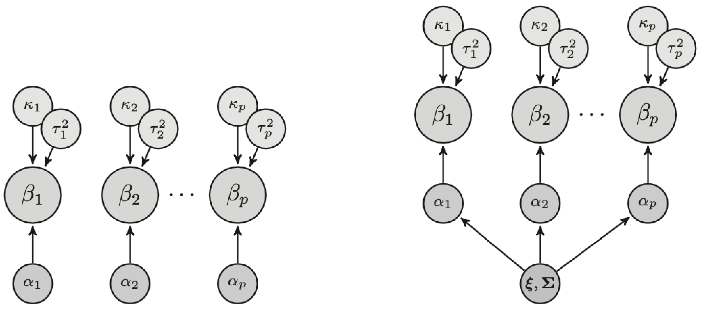
A Bayesian approach is completed by specification of model priors $p\left(\mathcal{M}\right)$ and parameter priors for each model $p\left(\mathsf{\beta }\right|\mathcal{M})$. Many kinds of priors can be considered. We follow our early preprint [11] as well as even earlier ideas from Polson and Ročková [10] and Hubin [41] and consider the independent spike-and-slab weight priors combined with independent Beta Binomial priors for the latent inclusion indicators. However, unlike earlier works, we introduce a more flexible t-distribution, allowing for “fat” tails for the slab components:

$$\begin{array}{cc}\hfill p\left({\beta }_{kj}^{\left(l\right)}\right|a_{\beta }^{\left(l\right)},b_{\beta }^{\left(l\right)},{\gamma }_{kj}^{\left(l\right)})=& {\gamma }_{kj}^{\left(l\right)}{t}_{2a_{\beta }^{\left(l\right)}}({\beta }_{kj}^{\left(l\right)};0,b_{\beta }^{\left(l\right)}/a_{\beta }^{\left(l\right)})+(1-{\gamma }_{kj}^{\left(l\right)}){\delta }_0\left({\beta }_{kj}^{\left(l\right)}\right),\hfill \end{array}$$

(3a)

$$\begin{array}{cc}\hfill p\left({\gamma }_{kj}^{\left(l\right)}\right)=& \mathrm{BetaBinomial}({\gamma }_{kj}^{\left(l\right)};1,a_{\psi }^{\left(l\right)},b_{\psi }^{\left(l\right)}).\hfill \end{array}$$

(3b)

Here, we have a $2a_{\beta }^{\left(l\right)}$ degrees of freedom parameter for the t-distribution with a zero mean and a variance of ${\sigma }_{\beta ,l}^2=b_{\beta }^{\left(l\right)}/a_{\beta }^{\left(l\right)}$. Further, ${\delta }_0(·)$ is the delta mass or “spike” at zero, whilst ${\psi }^{\left(l\right)}=a_{\psi }^{\left(l\right)}/\left(a_{\psi }^{\left(l\right)}+b_{\psi }^{\left(l\right)}\right)\in [0,1]$ is the prior probability for including the weight ${\beta }_{kj}^{\left(l\right)}$ into the model. We will refer to our model as the Latent Binary Bayesian Neural Network (LBBNN) model.

3. Bayesian Inference

3.1. Bayesian Model Averaging

The main goal of inference with uncertainty in both models and parameters is to infer the posterior marginal distribution of some parameter of interest $\Delta$ (for example, the distribution of a new observation $y^{*}$ conditional on new covariates ${\mathit{x}}^{*}$) based on data $\mathcal{D}$:

$$\begin{array}{c}\hfill p(\Delta |\mathcal{D})=\sum _{\mathcal{M}\in \mathsf{\Gamma }}p(\Delta |\mathcal{M},\mathcal{D})p\left(\mathcal{M}\right|\mathcal{D}),\end{array}$$

(4)

where $p(\Delta |\mathcal{M},\mathcal{D})={\int }_{\mathsf{\beta }}p(\Delta |\mathsf{\beta },\mathcal{M},\mathcal{D})p\left(\mathsf{\beta }\right|\mathcal{M},\mathcal{D})\mathrm{d}\mathsf{\beta }$ is a marginal posterior of some parameter $\Delta$ for model $\mathcal{M}$. Finally, $\mathsf{\Gamma }$ is the discrete space of all possible models addressed; for linear models, these models are defined by the combinations of included/excluded covariates, while for Bayesian neural networks, this space will consist of all architectures defined by inclusion/exclusion of every weight parameter of the network, allowing for the capturing of structural uncertainty. Further, $p\left(\mathcal{M}\right|\mathcal{D})$ are the marginal posterior model probabilities computed as

$$\begin{array}{c}\hfill p\left(\mathcal{M}\right|\mathcal{D})=\frac{p\left(\mathcal{D}\right|\mathcal{M}\left)p\right(\mathcal{M})}{{\sum }_{{\mathcal{M}}^{\prime }\in \mathsf{\Gamma }}p\left(\mathcal{D}\right|{\mathcal{M}}^{\prime })p\left({\mathcal{M}}^{\prime }\right)},\end{array}$$

(5)

and $p\left(\mathcal{D}\right|\mathcal{M})$ is the marginal likelihood of a model $\mathcal{M}$

$$\begin{array}{c}\hfill p\left(\mathcal{D}\right|\mathcal{M})={\int }_{\mathsf{\beta }}p\left(\mathcal{D}\right|\mathsf{\beta },\mathcal{M})p\left(\mathsf{\beta }\right|\mathcal{M})\mathrm{d}\mathsf{\beta }.\end{array}$$

(6)

This directly follows the definition of Bayesian model averaging from Raftery et al. [9] introduced in the context of linear models. Equations (4)–(6) can be combined into a single expression:

$$\begin{array}{c}\hfill p(\Delta |\mathcal{D})=\sum _{\mathcal{M}\in \mathsf{\Gamma }}{\int }_{\mathsf{\beta }}p(\Delta |\mathsf{\beta },\mathcal{M},\mathcal{D})p(\mathsf{\beta },\mathcal{M}|\mathcal{D})\mathrm{d}\mathsf{\beta }.\end{array}$$

(7)

Standard procedures for dealing with complex posteriors is to apply (reversible jump) Markov chain Monte Carlo (MCMC) methods, which involve simulations from $p(\mathsf{\beta },\mathcal{M}|\mathcal{D})$. But for the model defined by (1)–(3) with many hidden variables, such simulations become computationally infeasible.

3.2. Variational Approximation

As an alternative to MCMC, (7) can be directly approximated using a variational distribution as

$$\begin{array}{c}\hfill \tilde{p}(\Delta |\mathcal{D})=\sum _{\mathcal{M}\in \mathsf{\Gamma }}{\int }_{\mathsf{\beta }}p(\Delta |\mathsf{\beta },\mathcal{M},\mathcal{D})q_{\mathsf{\eta }}(\mathsf{\beta },\mathcal{M})\mathrm{d}\mathsf{\beta },\end{array}$$

(8)

where $q_{\mathsf{\eta }}(\mathsf{\beta },\mathcal{M})$ is selected from some suitable class of distributions $\left\{q_{\mathsf{\eta }}(\mathsf{\beta },\mathcal{M})\right\}$, parametrized by a set of variational parameters $\mathsf{\eta }$, that is simple to sample from. The variational distribution can potentially approximate the posterior well with appropriate choices of the parameters $\mathsf{\eta }$. The specification of $\mathsf{\eta }$ is typically obtained through the minimization of the Kullback–Leibler divergence from the variational family distribution to the posterior distribution:

$$\begin{array}{cc}\hfill \mathrm{KL}(q_{\mathsf{\eta }}(\mathsf{\beta },\mathcal{M})& \left|\right|p(\mathsf{\beta },\mathcal{M}|\mathcal{D}))=\sum _{\mathcal{M}\in \mathsf{\Gamma }}{\int }_{\mathsf{\beta }}{q}_{\mathsf{\eta }}(\mathsf{\beta },\mathcal{M})log\frac{q_{\mathsf{\eta }}(\mathsf{\beta },\mathcal{M})}{p(\mathsf{\beta },\mathcal{M}|\mathcal{D})}\mathrm{d}\mathsf{\beta },\hfill \end{array}$$

(9)

with respect to $\mathsf{\eta }$. Compared to standard variational inference approaches [16], the setting is extended to include the discrete model identifiers $\mathcal{M}$. For an optimal choice $\widehat{\mathsf{\eta }}$ of $\mathsf{\eta }$, inference on $\Delta$ is performed through Monte Carlo estimation of (8), inserting $\widehat{\mathsf{\eta }}$ for $\mathsf{\eta }$. The main challenge then becomes choosing a suitable variational family and a computational procedure for minimizing (9). Note that although this minimization is still a computational challenge, it will typically be much easier than directly obtaining samples from the true posterior. The final Monte Carlo estimation will be simple, provided the variational distribution $q_{\mathsf{\eta }}(\mathsf{\beta },\mathcal{M})$ is selected such that it is simple to sample from.

As in standard settings of variational inference, minimization of the divergence (9) is equivalent to maximization of the evidence lower bound (ELBO)

$$\begin{array}{cc}\hfill {\mathcal{L}}_{VI}\left(\mathsf{\eta }\right)=& \sum _{\mathcal{M}\in \mathsf{\Gamma }}{\int }_{\mathsf{\beta }}{q}_{\mathsf{\eta }}(\mathsf{\beta },\mathcal{M})logp\left(\mathcal{D}\right|\mathsf{\beta },\mathcal{M})\mathrm{d}\mathsf{\beta }-\mathrm{KL}\left(q_{\mathsf{\eta }}(\mathsf{\beta },\mathcal{M})\left|\right|p(\mathsf{\beta },\mathcal{M})\right)\hfill \end{array}$$

(10)

through the equality

$$\begin{array}{cc}\hfill {\mathcal{L}}_{VI}\left(\mathsf{\eta }\right)=& p\left(\mathcal{D}\right)-\mathrm{KL}\left(q_{\mathsf{\eta }}(\mathsf{\beta },\mathcal{M})\left|\right|p(\mathsf{\beta },\mathcal{M}|\mathcal{D})\right),\hfill \end{array}$$

which also shows that ${\mathcal{L}}_{VI}\left(\mathsf{\eta }\right)$ is a lower bound of the marginal likelihood $p\left(\mathcal{D}\right)$.

3.2.1. Mean-Field Approximations

We will consider a mean-field type variational family previously proposed for linear regression [43,44], which we extend to the LBBNN setting.

Assume

$$\begin{array}{c}\hfill q_{\mathsf{\eta }}(\mathsf{\beta },\mathcal{M})=\prod _{l=1}^{L-1}\prod _{j=1}^{p^{(l+1)}}\prod _{k=0}^{p^{\left(l\right)}}{q}_{{\kappa }_{kj}^{\left(l\right)},{\tau }_{kj}^{\left(l\right)}}\left({\beta }_{kj}^{\left(l\right)}\right|{\gamma }_{kj}^{\left(l\right)})q_{{\alpha }_{kj}^{\left(l\right)}}\left({\gamma }_{kj}^{\left(l\right)}\right),\end{array}$$

(11)

where

$$\begin{array}{cc}\hfill q_{{\kappa }_{kj}^{\left(l\right)},{\tau }_{kj}^{\left(l\right)}}\left({\beta }_{kj}^{\left(l\right)}|{\gamma }_{kj}^{\left(l\right)}\right)=& {\gamma }_{kj}^{\left(l\right)}\mathcal{N}({\beta }_{kj}^{\left(l\right)};{\kappa }_{kj}^{\left(l\right)},{{\tau }^2}_{kj}^{\left(l\right)})+(1-{\gamma }_{kj}^{\left(l\right)}){\delta }_0\left({\beta }_{kj}^{\left(l\right)}\right),\hfill \end{array}$$

(12)

and

$$\begin{array}{cc}\hfill q_{{\alpha }_{kj}^{\left(l\right)}}\left({\gamma }_{kj}^{\left(l\right)}\right)=& \mathrm{Bernoulli}({\gamma }_{kj}^{\left(l\right)};{\alpha }_{kj}^{\left(l\right)}).\hfill \end{array}$$

(13)

With probability, ${\alpha }_{kj}^{\left(l\right)}\in [0,1]$, the posterior of parameters of weight ${\beta }_{kj}^{\left(l\right)}$ will be approximated by a normal distribution with some mean and variance (“slab”), and otherwise, the weight is put to zero. Thus, ${\alpha }_{kj}^{\left(l\right)}$ will approximate the marginal posterior inclusion probability of the weight ${\beta }_{kj}^{\left(l\right)}$. Here, $\mathsf{\eta }=\{{({\kappa }_{kj}^{\left(l\right)},{\tau }^2}_{kj}^{\left(l\right)},{\alpha }_{kj}^{\left(l\right)}),l=1,\dots ,L-1,k=0,\dots ,p^{\left(l\right)},$ $j=1,\dots ,p^{(l+1)}\}$. This approximation is graphically illustrated in the left panel of Figure 1.

A similar variational distribution has also been considered within BNN through the dropout approach [45]. For dropout, however, the final network is dense but trained through a Monte Carlo average of sparse networks. In our approach, the target distribution is different in the sense of including the binary variables $\left\{{\gamma }_{kj}^{\left(l\right)}\right\}$ as part of the model. Hence, our marginal inclusion probabilities can serve as a particular case of dropout rates, with a proper probabilistic interpretation in terms of structural model uncertainty.

3.2.2. Dependence Structures in the Variational Approximation

The mean-field variational distribution (11)–(13) can be seen as a rather crude approximation, which completely ignores all posterior dependence between the model structures or parameters. Consequently, the resulting conclusions can be misleading or inaccurate, as the posterior probability of one weight might be highly affected by the inclusion of others. Such a dependence structure can be built into the variational approximation either through the $\gamma$’s or through the $\beta$’s (or both), leading to an extension of the mean-field approach. Here, we only consider dependence structures in the inclusion variables. We still assume independence between layers. Within layers, we introduce a dependence structure by defining ${\mathsf{\alpha }}^{\left(l\right)}=\left\{{\alpha }_{kj}^{\left(l\right)}\right\}$ now to be a stochastic vector, which, on logit-scale, follows a multivariate normal distribution:

$$\begin{array}{c}\hfill \mathrm{logit}\left({\mathsf{\alpha }}^{\left(l\right)}\right)\sim \mathrm{MVN}(\mathrm{logit}\left({\mathsf{\alpha }}^{\left(l\right)}\right);{\mathsf{\xi }}^{\left(l\right)},{\mathsf{\Sigma }}^{\left(l\right)}).\end{array}$$

(14)

Here, either a full covariance matrix ${\mathsf{\Sigma }}^{\left(l\right)}$ or a low-rank parametrization for the covariance is possible. For the latter, ${\mathsf{\Sigma }}^{\left(l\right)}={\mathit{F}}^{\left(l\right)}{{\mathit{F}}^{\left(l\right)}}^T+{\mathit{D}}^{\left(l\right)}$, with ${\mathit{F}}^{\left(l\right)}$ being the factor part of a low-rank form of the covariance matrix, and ${\mathit{D}}^{\left(l\right)}$ is the diagonal part of the low-rank form of the covariance matrix. This drastically reduces the number of parameters and allows for efficient computations of the determinant and inverse matrix. Under the parametrization (12)–(14), the parameters $\{{\mathsf{\xi }}^{\left(l\right)},l=1,\dots ,L-1\}$ and $\{{\mathsf{\Sigma }}^{\left(l\right)},l=1,\dots ,L-1\}$ are added to the parameter vector $\mathsf{\eta }$. This approximation is illustrated in the right panel of Figure 1.

3.3. Optimization by Stochastic Gradient

By plugging in the explicit expression for the Kullback–Leibler divergence from (9) in (10), we can rewrite the ELBO (10) as

$$\begin{array}{cc}\hfill {\mathcal{L}}_{VI}\left(\mathsf{\eta }\right)=& \sum _{\mathcal{M}\in \mathsf{\Gamma }}{\int }_{\mathsf{\beta }}{q}_{\mathsf{\eta }}(\mathsf{\beta },\mathcal{M})[logp\left(\mathcal{D}\right|\mathsf{\beta },\mathcal{M})-log\frac{q_{\mathsf{\eta }}(\mathsf{\beta },\mathcal{M})}{p(\mathsf{\beta },\mathcal{M})}]\mathrm{d}\mathsf{\beta },\hfill \end{array}$$

(15)

which we need to minimize with respect to $\mathsf{\eta }$. Due to the huge computational cost in the computation of gradients when $\mathsf{\Gamma }$ and $\mathcal{D}$ are large, stochastic gradient methods using Monte Carlo estimates for obtaining unbiased estimates of the gradients have become the standard approach for variational inference in such situations. Both the reparametrization trick and minibatching [16,46] are further applied.

Another complication in our setting is the discrete nature of $\mathcal{M}$. Following Gal et al. [47], we relax the Bernoulli distribution (13) with the Concrete distribution:

$$\begin{array}{c}\hfill \tilde{\gamma }={\gamma }_{tr}(\nu ,\delta ;\alpha )=\mathrm{sigmoid}(\left(\mathrm{logit}\left(\alpha \right)-\mathrm{logit}\left(\nu \right))/\delta \right),\nu \sim \mathrm{Unif}[0,1],\end{array}$$

(16)

where $\delta$ is a tuning parameter, which is selected to take some small value. In the zero limit, $\tilde{\gamma }$ reduces to a Bernoulli$\left(\alpha \right)$ variable. Combined with the reparametrization of the $\beta$’s,

$$\begin{array}{c}\hfill \beta ={\beta }_{tr}(\epsilon ;\kappa ,\tau )=\kappa +\tau \epsilon ,\epsilon \sim N(0,1),\end{array}$$

(17)

define the following approximation to the ELBO:

$$\begin{array}{cc}\hfill {\mathcal{L}}_{VI}^{\delta }\left(\mathsf{\eta }\right):={\int }_{\mathsf{\nu }}{\int }_{\mathsf{\epsilon }}{q}_{\mathsf{\nu },\mathsf{\epsilon }}(\mathsf{\nu },\mathsf{\epsilon })[& logp\left(\mathcal{D}\right|{\beta }_{tr}(\mathsf{\epsilon },\mathsf{\kappa },\mathsf{\tau }),{\gamma }_{tr}(\mathsf{\nu },\mathsf{\alpha },\delta ))-\hfill \\ \hfill & log\frac{q_{\mathsf{\eta }}({\beta }_{tr}(\mathsf{\epsilon },\mathsf{\kappa },\mathsf{\tau }),{\gamma }_{tr}(\mathsf{\nu },\mathsf{\alpha },\delta ))}{p({\beta }_{tr}(\mathsf{\epsilon },\mathsf{\kappa },\mathsf{\tau }),{\gamma }_{tr}(\mathsf{\nu },\mathsf{\alpha },\delta ))}]\mathrm{d}\mathsf{\epsilon }\mathrm{d}\mathsf{\nu },\hfill \end{array}$$

(18)

where the transformations on vectors are performed elementwise. Further, due to $\mathrm{d}\mathsf{\epsilon }\mathrm{d}\mathsf{\nu }$ not depending on $\mathsf{\eta }$, we can change the order of integration and differentiation when taking the gradient of ${\mathcal{L}}_{VI}^{\delta }\left(\mathsf{\eta }\right)$:

$$\begin{array}{cc}\hfill {\nabla }_{\mathsf{\eta }}{\mathcal{L}}_{VI}^{\delta }\left(\mathsf{\eta }\right)={\int }_{\mathsf{\nu }}{\int }_{\mathsf{\epsilon }}{q}_{\mathsf{\nu },\mathsf{\epsilon }}(\mathsf{\nu },\mathsf{\epsilon }){\nabla }_{\mathsf{\eta }}[& logp\left(\mathcal{D}\right|{\beta }_{tr}(\mathsf{\epsilon },\mathsf{\kappa },\mathsf{\tau }),{\gamma }_{tr}(\mathsf{\nu },\mathsf{\alpha },\delta )-\hfill \\ \hfill & log\frac{q_{\mathsf{\eta }}({\beta }_{tr}(\mathsf{\epsilon },\mathsf{\kappa },\mathsf{\tau }),{\gamma }_{tr}(\mathsf{\nu },\mathsf{\alpha },\delta ))}{p({\beta }_{tr}(\mathsf{\epsilon },\mathsf{\kappa },\mathsf{\tau }),{\gamma }_{tr}(\mathsf{\nu },\mathsf{\alpha },\delta ))}]\mathrm{d}\mathsf{\epsilon }\mathrm{d}\mathsf{\nu }.\hfill \end{array}$$

(19)

An unbiased estimator of ${\nabla }_{\mathsf{\eta }}{\mathcal{L}}_{VI}^{\delta }\left(\mathsf{\eta }\right)$ is then given in Proposition 1.

Proposition 1.

Assume $\left({\mathsf{\nu }}^{\left(m\right)},{\mathsf{\eta }}^{\left(m\right)}\right)\sim q_{\mathsf{\nu },\mathsf{\epsilon }}(\mathsf{\nu },\mathsf{\eta })$ for all $m=1,\dots ,M$, and S is a random subset of indices $\{1,\dots ,n\}$ of size N. Also, assume the observations to be conditionally independent. Then, for any $\delta >0$, an unbiased estimator for the gradient of ${\mathcal{L}}_{VI}^{\delta }\left(\mathsf{\eta }\right)$ is given by

$$\begin{array}{cc}\hfill {\tilde{\nabla }}_{\mathsf{\eta }}{\mathcal{L}}_{VI}^{\delta }\left(\mathsf{\eta }\right)=\frac{1}{M}\sum _{m=1}^M[& \frac{n}{N}\sum _{i\in S}{\nabla }_{\mathsf{\eta }}logp\left({\mathit{y}}_{\mathit{i}}\right|{\mathit{x}}_{\mathit{i}},{\beta }_{tr}({\mathsf{\epsilon }}^{\left(m\right)},\mathsf{\kappa },\mathsf{\tau }),{\gamma }_{tr}({\mathsf{\nu }}^{\left(m\right)},\mathsf{\alpha },\delta ))-\hfill \\ \hfill & {\nabla }_{\mathsf{\eta }}log\frac{q_{\mathsf{\eta }}({\beta }_{tr}({\mathsf{\epsilon }}^{\left(m\right)},\mathsf{\kappa },\mathsf{\tau }),{\gamma }_{tr}({\mathsf{\nu }}^{\left(m\right)},\mathsf{\alpha },\delta ))}{p({\beta }_{tr}({\mathsf{\epsilon }}^{\left(m\right)},\mathsf{\kappa },\mathsf{\tau }),{\gamma }_{tr}({\mathsf{\nu }}^{\left(m\right)},\mathsf{\alpha },\delta ))}].\hfill \end{array}$$

(20)

Proof. 

From (19) we have that

$$\begin{array}{c}\hfill \frac{1}{M}\sum _{m=1}^M{\nabla }_{\mathsf{\eta }}\left[logp\left(\mathcal{D}\right|{\beta }_{tr}({\mathsf{\epsilon }}^{\left(m\right)},\mathsf{\kappa },\mathsf{\tau }),{\gamma }_{tr}({\mathsf{\nu }}^{\left(m\right)},\mathsf{\alpha },\delta )-log\frac{q_{\mathsf{\eta }}({\beta }_{tr}({\mathsf{\epsilon }}^{\left(m\right)},\mathsf{\kappa },\mathsf{\tau }),{\gamma }_{tr}({\mathsf{\nu }}^{\left(m\right)},\mathsf{\alpha },\delta ))}{p({\beta }_{tr}({\mathsf{\epsilon }}^{\left(m\right)},\mathsf{\kappa },\mathsf{\tau }),{\gamma }_{tr}(\mathsf{\nu }{,}^{\left(m\right)},\mathsf{\alpha },\delta ))}\right]\end{array}$$

is an unbiased estimate of the gradient. Further, since we assume the observations to be conditionally independent, we have

$$\begin{array}{c}\hfill {\nabla }_{\mathsf{\eta }}logp\left(\mathcal{D}\right|{\beta }_{tr}(\mathsf{\epsilon },\mathsf{\kappa },\mathsf{\tau }),{\gamma }_{tr}(\mathsf{\nu },\mathsf{\alpha },\delta ))=\sum _{i=1}^n{\nabla }_{\mathsf{\eta }}logp\left({\mathit{y}}_i\right|{\mathit{x}}_i;{\beta }_{tr}(\mathsf{\epsilon },\mathsf{\kappa },\mathsf{\tau }),{\gamma }_{tr}(\mathsf{\nu },\mathsf{\alpha },\delta )),\end{array}$$

for which an unbiased estimator can be constructed through a random subset, showing the result.    □

Algorithm 1 describes one iteration of a doubly stochastic variational inference approach, where updating is performed on the parameters for the case of mean field assumption (for simplicity). The term double stochastic refers to the fact that sampling in the unbiased gradient approximation is performed both on parameters and subsets of data, which we have shown to be possible through Proposition 1. In Algorithm 1, the set $\mathcal{B}$ is the collection of all combinations $j,k,l$ in the network. The matrix of learning rates $\mathit{A}$ will always be diagonal, allowing for different step sizes on the parameters involved. Following Blundell et al. [16], constraints of ${\tau }_{kj}^{\left(l\right)}$ are incorporated by means of the reparametrization ${\tau }_{kj}^{\left(l\right)}=log(1+exp\left({\rho }_{kj}^{\left(l\right)}\right))$, where ${\rho }_{kj}^{\left(l\right)}\in \mathcal{R}$. Typically, updating is performed over a full epoch, in which case the observations are divided into $n/N$ subsets, and updating is performed sequentially over all subsets.  

Algorithm 1 Doubly stochastic variational inference step

sample N indices uniformly from $\{1,\dots ,n\}$ defining S; for m in $\{1,\dots ,M\}$ do    for $(k,j,l)\in \mathcal{B}$ do      sample ${\nu }_{kl}^{\left(l\right)}\sim \mathrm{Unif}[0,1]$ and ${\epsilon }_{kj}^{\left(l\right)}\sim N(0,1)$    end for end for calculate ${\tilde{\nabla }}_{\mathsf{\eta }}{\mathcal{L}}_{VI}^{\delta }\left(\mathsf{\eta }\right)$ according to (20) update $\mathsf{\eta }\leftarrow \mathsf{\eta }+\mathit{A}{\tilde{\nabla }}_{\mathsf{\eta }}{\mathcal{L}}_{VI}^{\delta }\left(\mathsf{\eta }\right)$

In casthe e of the dependence structure (14), ${\mathsf{\alpha }}^{\left(l\right)}$ is sampled instead, while ${\mathsf{\xi }}^{\left(l\right)}$ and the components of ${\mathsf{\Sigma }}^{\left(l\right)}$ go into $\mathsf{\eta }$. Also, for the MVN and LFMVN, the reparametrization trick is performed for their parameters using the default representations that are available out-of-the box in PyTorch probabilities (https://pytorch.org/docs/stable/distributions.html, accessed on 25 January 2024). Lastly, in the mean-field case, constraints on ${\alpha }_{kj}^{\left(l\right)}$ are incorporated by means of the reparametrization ${\alpha }_{kj}^{\left(l\right)}={\left(1+exp(-{\omega }_{kj}^{\left(l\right)})\right)}^{-1}$ with ${\omega }_{kj}^{\left(l\right)}\in \mathcal{R}$.

Note that in the suggested algorithm, partial derivatives concerning marginal inclusion probabilities, as well as mean and standard deviation terms of the weights, can be calculated by the usual backpropagation algorithm.

3.4. Prediction

Once the estimates $\widehat{\mathsf{\eta }}$ of the parameters $\mathsf{\eta }$ of the variational approximating distribution are obtained, we go back to the original discrete model for $\mathcal{M}$ (setting $\delta =0$). Then, there are several ways to proceed with predictive inference. We list these below.

3.4.1. Fully Bayesian Model Averaging

In this case, define a Monte Carlo approximation to (8) by

$$\widehat{p}(\Delta |\mathcal{D})=\frac{1}{R}\sum _{r=1}^{R}p(\Delta |{\mathsf{\beta }}^r,{\mathcal{M}}^r),$$

(21)

where $({\mathsf{\beta }}^r,{\mathcal{M}}^r)\sim q_{\widehat{\mathsf{\eta }}}(\mathsf{\beta },\mathcal{M})$, $r=1,\dots ,R$. This procedure takes uncertainty in both the model structure $\mathcal{M}$ and the parameters $\mathsf{\beta }$ into account in a formal Bayesian setting. A bottleneck of this approach is that we have to both sample from a huge approximate posterior distribution of parameters and models and keep all of the components of $\widehat{\mathsf{\eta }}$ stored during the prediction phase, which might be computationally and memory inefficient.

3.4.2. The Posterior Mean Based Model [48]

In this case, we put ${\beta }_{kj}^{\left(l\right)}=\widehat{E}\left\{{\beta }_{kj}^{\left(l\right)}\right|\mathcal{D}\}$, where

$$\begin{array}{cc}\hfill E\left\{{\beta }_{kj}^{\left(l\right)}\right|\mathcal{D}\}=& p({\gamma }_{kj}^{\left(l\right)}=1|\mathcal{D})E\left[{\beta }_{kj}^{\left(l\right)}|{\gamma }_{kj}^{\left(l\right)}=1,\mathcal{D}\right]\approx {\widehat{\alpha }}_{kj}^{\left(l\right)}{\widehat{\kappa }}_{kj}^{\left(l\right)}.\hfill \end{array}$$

Here, ${\widehat{\alpha }}_{kj}^{\left(l\right)}$ is the estimate of ${\alpha }_{kj}^{\left(l\right)}$ obtained through the variational inference procedure. This approach specifies one dense model $\widehat{\mathcal{M}}$ with no sparsification. At the same time, no sampling is needed.

3.4.3. The Median Probability Model [49]

This approach is based on the notion of a median probability model, which has been shown to be optimal in terms of predictions in the context of simple linear models. Here, we set ${\gamma }_{kj}^{\left(l\right)}=\mathrm{I}({\widehat{\alpha }}_{kj}^{\left(l\right)}>0.5)$, while ${\beta }_{kj}^{\left(l\right)}\sim {\gamma }_{kj}^{\left(l\right)}N({\widehat{\kappa }}_{kj}^{\left(l\right)},{\widehat{\tau }}_{kj}^{2\left(l\right)})$. A model averaging approach similar to (21) is then applied. Within this approach, we significantly sparsify the network and only sample from the distributions of those weights that have marginal inclusion probabilities above 0.5.

3.4.4. Median Probability Model-Based Inference Combined with Parameter Posterior Mean

Here, again, we set ${\gamma }_{kj}^{\left(l\right)}=\mathrm{I}({\widehat{\alpha }}_{kj}^{\left(l\right)}>0.5)$, but now, we use ${\beta }_{kj}^{\left(l\right)}={\gamma }_{kj}^{\left(l\right)}{\widehat{\kappa }}_{kj}^{\left(l\right)}$. Similar to the posterior mean-based model, no sampling is needed, but in addition, we only need to store the variational parameters of $\widehat{\mathsf{\eta }}$ corresponding to marginal inclusion probabilities above 0.5. Hence, we significantly sparsify the BNN of interest and reduce the computational cost of the predictions drastically.

3.4.5. Post-Training

Once it is decided to make inference based on a selected model, one might make several additional iterations of the training algorithm concerning the parameters of the models, having the architecture-related parameters fixed. This might give additional improvements in terms of the quality of inference as well as make the training steps much easier since the number of parameters is reduced dramatically. This is so since one does not have to estimate marginal inclusion probabilities $\mathsf{\alpha }$ any longer. Moreover, the number of weights ${\beta }_{jk}^{\left(l\right)}$’s corresponding to ${\gamma }_{jk}^{\left(l\right)}=1$ that the inference is based on is typically significantly reduced due to the sparsity induced by using the selected median probability model. It is also possible to keep the ${\alpha }_{jk}^{\left(l\right)}$’s fixed but still allow the ${\gamma }_{jk}^{\left(l\right)}$’s to be random.

4. Applications

In-depth studies of the suggested variational approximations in the context of linear regression models have been performed in earlier studies, including multiple synthetic and real data examples with the aims of both recovering meaningful relations and predictions [44,50]. The results from these studies show that the approximations based on the suggested variational family distributions are reasonably precise and indeed scalable but can be biased. We will not address toy examples and simulation-based examples in this article and rather refer the curious readers to the very detailed and comprehensive studies in the references mentioned above, whilst we will address some more complex examples here. In particular, we will address the classification of MNIST [51] and fashion-MNIST ([52] FMNIST) images, as well as the PHONEME data [53]. Both MNIST and FMNIST datasets comprise 70,000 grayscale images (size 28x28) from 10 categories (handwritten digits from 0 to 9, and “Top”, “Trouser”, “Pullover”, “Dress”, “Coat”, “Sandal”, “Shirt”, “Sneaker”, “Bag” and “Ankle Boot” Zalando’s fashion items, respectively), with 7000 images per category. The training sets consist of 60,000 images, and the test sets have 10,000 images. For the PHONEME dataset, we have 256 covariates and 5 classes in the responses. In this dataset, we have 3500 observations in the training set and 1000 observations in the test set. The PHONEME data are extracted from the TIMIT database (TIMIT Acoustic-Phonetic Continuous Speech Corpus, NTIS, US Dept of Commerce), which is a widely used resource for research in speech recognition. This dataset was formed by selecting five phonemes for classification based on a digitized speech from this database. The phonemes are transcribed as follows: “sh” as in “she”, “dcl” as in “dark”, “iy” as the vowel in “she”, “aa” as the vowel in “dark” and “ao” as the first vowel in “water”. Additionally, in the Appendix to the paper, we report results on the standard tabular UCI datasets https://archive.ics.uci.edu/datasets (accessed on 25 January 2024), including credit approval data, bank marketing data, adult census data, dry beans data, pistachio data and raisins data.

4.1. Experimental Design

For the three datasets addressed in the main part of the paper, we use a feed-forward neural network with the ReLU activation function and multinomially distributed observations. For the two first examples, we have 10 classes and 784 input explanatory variables (pixels), while for the third one, we have 256 input variables and 5 classes. In all three cases, the network has 2 hidden layers with 400 and 600 neurons, correspondingly. Priors for the parameters and model indicators were chosen according to (3). The inference was performed using the suggested doubly stochastic variational inference approach (Algorithm 1) on 250 epochs with a batch size of 100. M was set to 1 to reduce computational costs and because this choice of M is argued to be sufficient in combination with the reparametrization trick [38]. Up to 20 first epochs were used for pre-training of the models and parameters, as well as empirically (aka Empirical Bayes) estimating the hyperparameters of the priors ($a_{\psi },b_{\psi },a_{\beta },b_{\beta }$) by adding them into the computational graph. After that, the main training cycle began (with fixed hyperparameters on the priors). We used the ADAM stochastic gradient ascent optimization [54] with the diagonal matrix $\mathit{A}$ in Algorithm 1 and the diagonal elements specified in

Table 1. Specifications of diagonal elements of $\mathit{A}$ matrices for the step sizes of optimization routines for LBBNN-SSP-MF and LBBNN-SSP-MVN; see the Abbreviations section for futher detail. Note that $A_{\omega }$ is only used in LBBNN-SSP-MF, while $A_{\xi }$ and $A_{\mathsf{\Sigma }}$ are only used in LBBNN-SSP-MVN. For tuning parameters of LBBNN-SSP-LFMVN, see Table A1 in the Appendix to the paper.

	${\mathit{A}}_{\mathit{\beta }}$, ${\mathit{A}}_{\mathit{\rho }}$	${\mathit{A}}_{\mathit{\xi }}$	${\mathit{A}}_{\mathit{\omega }}$	${\mathit{A}}_{\mathsf{\Sigma }}$	${\mathit{A}}_{{\mathit{a}}_{\mathit{\psi }}}$, ${\mathit{A}}_{{\mathit{b}}_{\mathit{\psi }}}$	${\mathit{A}}_{{\mathit{a}}_{\mathit{\beta }}}$, ${\mathit{A}}_{{\mathit{b}}_{\mathit{\beta }}}$
Pre-training	1.00 × ${10}^{-4}$	1.00 × ${10}^{-1}$	1.00 × ${10}^{-1}$	1.00 × ${10}^{-1}$	1.00 × ${10}^{-3}$	1.00 × ${10}^{-5}$
Training	1.00 × ${10}^{-4}$	1.00 × ${10}^{-2}$	1.00 × ${10}^{-4}$	1.00 × ${10}^{-4}$	0.00	0.00
Post-training	1.00 × ${10}^{-4}$	0.00	0.00	0.00	0.00	0.00

and

Table A3. Performance metrics for the FMNIST data, in addition to Table 3 using low factor MVN.

Prediction		Model-Prior-Method	R	All cl Acc	0.95 Threshold		Dens. Level	Epo. Time
$\mathcal{M}$	$\mathsf{\beta }$				Acc	Num.cl
SIM	SIM	LBBNN-SSP-LFMVN	1	0.849 (0.845,0.853)	-	-	0.456	12.949
SIM	SIM		10	0.876 (0.874,0.880)	0.996	4485	1.000	12.949
ALL	EXP		1	0.864 (0.862,0.867)	-	-	1.000	12.949
MED	SIM		1	0.849 (0.844,0.852)	-	-	0.455	12.949
MED	SIM		10	0.877 (0.875,0.878)	0.996	4486	0.455	12.949
MED	EXP		1	0.862 (0.858,0.864)	-	-	0.455	12.949

for pre-training, and the main training stage. After 250 training epochs, post-training was performed. When post-training the parameters, either with fixed marginal inclusion probabilities or with the median probability model, we ran an additional 50 epochs of the optimization routine, with $\mathit{A}$ specified in the bottom rows of Table 1 and

Table A1. Specifications of diagonal elements of $\mathit{A}$ matrix for LBBNN-SSP-LFMVN.

	${\mathit{A}}_{\mathit{\beta }}$, ${\mathit{A}}_{\mathit{\rho }}$	${\mathit{A}}_{\mathit{\xi }}$	${\mathit{A}}_{\mathit{\omega }}$	${\mathit{A}}_{\mathsf{\Sigma }}$	${\mathit{A}}_{{\mathit{a}}_{\mathit{\psi }}}$, ${\mathit{A}}_{{\mathit{b}}_{\mathit{\psi }}}$	${\mathit{A}}_{{\mathit{a}}_{\mathit{\beta }}}$, ${\mathit{A}}_{{\mathit{b}}_{\mathit{\beta }}}$
Pre-training	1.00 × ${10}^{-4}$	1.00 × ${10}^{-2}$	-	1.00 × ${10}^{-2}$	1.00 × ${10}^{-2}$	1.00 × ${10}^{-5}$
Training	1.00 × ${10}^{-4}$	1.00 × ${10}^{-4}$	-	1.00 × ${10}^{-4}$	0.00	0.00
Post-training	1.00 × ${10}^{-4}$	0.00	-	0.00	0.00	0.00

. For the fully Bayesian model averaging approach, we used both $R=1$ and $R=10$. Even though $R=1$ can give a poor Monte Carlo estimate of the prediction distribution, it can be of interest due to high sparsification. All the PyTorch implementations used in the experiments are available in our GitHub repository (https://github.com/aliaksah/Variational-Inference-for-Bayesian-Neural-Networks-under-Model-and-Parameter-Uncertainty (accessed on 25 January 2024)).

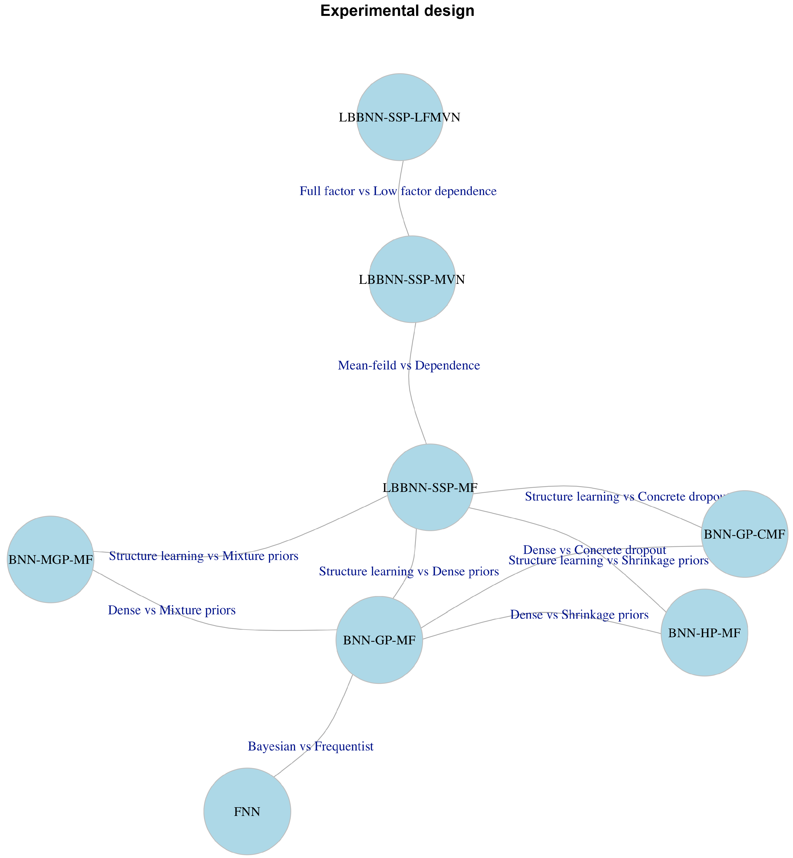
We report results for our model LBBNN applied with the spike-and-slab priors (SSP) combined with variational inference based on Mean-Field (MF), MVN (MVN) and Low Factor MVN (for LFMVN, the predictions’ results are reported in the Appendix) dependence structures between the latent indicators. We use the combined names LBBNN-SSP-MF, LBBNN-SSP-MVN and LBBNN-SSP-LFMVN, respectively, to denote the combination of model, prior and variational distribution.

In addition, we also used several relevant baselines. In particular, we addressed a standard Dense BNN with Gaussian priors and mean-field variational inference [37], denoted as BNN-GP-MF. This model is important in measuring how predictive power is changed due to the introduction of sparsity. Furthermore, we report the results for a Dense BNN with mixture priors (BNN-MGP-MF), with two Gaussian components of the mixtures [16], with probabilities of 0.5 for each and variances equal to 1 and $2.479\times {10}^{-3}$, correspondingly. Additionally, we have addressed two popular sparsity-inducing approaches, in particular, a dense network with Concrete dropout (BNN-GP-CMF) [47] and a dense network with Horseshoe priors (BNN-HP-MF) [22]. Finally, a frequentist fully connected neural network (FNN) (with posthoc weight pruning) was used as a more basic baseline. We only report the results for FNN in the Appendix to make the experimental design cleaner. All of the baseline methods (including the FNN) also have 2 hidden layers with 400 and 600 neurons, respectively, corresponding to three layers of weights. They were trained for 250 epochs with an Adam optimizer (with a learning rate $a=1.00\times {10}^{-4}$ for all involved parameters) and a batch size equal to 100. For the BNN with Horseshoe priors, we are reporting statistics separately before and after ad-hoc pruning (PRN) of the weights. Post-training (when necessary) was performed for an additional 50 epochs. For FNN, for all three experiments, we performed weight and neuron pruning [55] to have the same sparsity levels as those obtained by the Bayesian approaches to make them directly comparable. Pruning of FNN was based on removing the corresponding share of weights/neurons having the smallest magnitude (absolute value). No uncertainty was taken into consideration and neither was structure learning considered for FNNs. Main results for the specific baselines will be reported in

Table 2. Performance metrics for the MNIST data for the compared approaches. All results are medians across 10 repeated experiments (with min and max included in parentheses). Our methods’ names are bold. No post-training is used. For further details, see the Abbreviations section.

Prediction		Model-Prior-Method	R	All cl Acc	0.95 Threshold		Dens. Level	Epo. Time
$\mathcal{M}$	$\mathsf{\beta }$				Acc	Num.cl
SIM	SIM	LBBNN-SSP-MF	1	0.968 (0.966,0.970)	-	-	0.090	8.363
SIM	SIM		10	0.981 (0.979,0.982)	0.999	8322	1.000	8.363
ALL	MEA		1	0.981 (0.980,0.983)	-	-	1.000	8.363
MED	SIM		1	0.969 (0.968,0.974)	-	-	0.079	8.363
MED	SIM		10	0.980 (0.979,0.982)	0.999	8444	0.079	8.363
MED	MEA		1	0.981 (0.980,0.983)	-	-	0.079	8.363
SIM	SIM	LBBNN-SSP-MVN	1	0.965 (0.964,0.966)	-	-	0.180	9.651
SIM	SIM		10	0.978 (0.976,0.979)	1.000	7818	1.000	9.651
ALL	MEA		1	0.978 (0.976,0.980)	-	-	1.000	9.651
MED	SIM		1	0.968 (0.966,0.969)	-	-	0.163	9.651
MED	SIM		10	0.977 (0.975,0.979)	1.000	7928	0.163	9.651
MED	MEA		1	0.974 (0.972,0.976)	-	-	0.163	9.651
ALL	SIM	BNN-GP-MF	1	0.965 (0.965,0.966)	-	-	1.000	5.094
ALL	SIM		10	0.984 (0.982,0.985)	0.999	8477	1.000	5.094
ALL	MEA		1	0.984 (0.982,0.985)	-	-	1.000	5.094
ALL	SIM	BNN-MGP-MF	1	0.965 (0.964,0.967)	-	-	1.000	5.422
ALL	SIM		10	0.982 (0.981,0.983)	0.999	8329	1.000	5.422
ALL	MEA		1	0.983 (0.981,0.984)	-	-	1.000	5.422
SIM	SIM	BNN-GP-CMF	1	0.982 (0.894,0.984)	-	-	0.226	3.477
SIM	SIM		10	0.984 (0.896,0.986)	0.995	9581	1.000	3.477
ALL	MEA		1	0.984 (0.893,0.986)	-	-	1.000	3.477
SIM	SIM	BNN-HP-MF	1	0.964 (0.962,0.967)	-	-	1.000	4.254
SIM	SIM		10	0.982 (0.981,0.983)	1.000	0003	1.000	4.254
ALL	MEA		1	0.966 (0.963,0.968)	-	-	1.000	4.254
PRN	SIM		1	0.965 (0.962,0.969)	-	-	0.194	4.254
PRN	SIM		10	0.982 (0.981,0.983)	1.000	0002	0.194	4.254
PRN	MEA		1	0.965 (0.963,0.968)	-	-	0.194	4.254

,

Table 3. Performance metrics for the FMNIST data for the compared approaches. For further details, see the caption of Table 2.

Prediction		Model-Prior-Method	R	All cl Acc	0.95 Threshold		Dens. Level	Epo. Time
$\mathcal{M}$	$\mathsf{\beta }$				Acc	Num.cl
SIM	SIM	LBBNN-SSP-MF	1	0.864 (0.861,0.866)	-	-	0.120	7.969
SIM	SIM		10	0.883 (0.881,0.886)	0.995	4946	1.000	7.969
ALL	MEA		1	0.882 (0.879,0.887)	-	-	1.000	7.969
MED	SIM		1	0.867 (0.864,0.871)	-	-	0.108	7.969
MED	SIM		10	0.883 (0.880,0.886)	0.995	5025	0.108	7.969
MED	MEA		1	0.880 (0.877,0.886)	-	-	0.108	7.969
SIM	SIM	LBBNN-SSP-MVN	1	0.858 (0.854,0.859)	-	-	0.156	9.504
SIM	SIM		10	0.879 (0.874,0.880)	0.995	4503	1.000	9.504
ALL	MEA		1	0.875 (0.873,0.876)	-	-	1.000	9.504
MED	SIM		1	0.865 (0.860,0.866)	-	-	0.129	9.504
MED	SIM		10	0.877 (0.875,0.879)	0.995	4694	0.129	9.504
MED	MEA		1	0.871 (0.868,0.875)	-	-	0.129	9.504
ALL	SIM	BNN-GP-MF	1	0.864 (0.863,0.866)	-	-	1.000	5.368
ALL	SIM		10	0.893 (0.890,0.894)	0.997	5089	1.000	5.368
ALL	MEA		1	0.886 (0.882,0.888)	-	-	1.000	5.368
ALL	SIM	BNN-MGP-MF	1	0.867 (0.866,0.868)	-	-	1.000	4.803
ALL	SIM		10	0.893 (0.892,0.897)	0.996	5151	1.000	4.803
ALL	MEA		1	0.888 (0.885,0.890)	-	-	1.000	4.803
SIM	SIM	BNN-GP-CMF	1	0.896 (0.820,0.902)	-	-	0.094	3.369
SIM	SIM		10	0.897 (0.823,0.901)	0.942	8825	1.000	3.369
ALL	MEA		1	0.896 (0.821,0.901)	-	-	1.000	3.369
SIM	SIM	BNN-HP-MF	1	0.864 (0.863,0.869)	-	-	1.000	4.613
SIM	SIM		10	0.887 (0.886,0.889)	1.000	0181	1.000	4.613
ALL	MEA		1	0.867 (0.861,0.868)	-	-	1.000	4.613
PRN	SIM		1	0.865 (0.860,0.868)	-	-	0.302	4.613
PRN	SIM		10	0.887 (0.884,0.888)	1.000	0179	0.302	4.613
PRN	MEA		1	0.865 (0.862,0.869)	-	-	0.302	4.613

and

Table 4. Performance metrics for the PHONEME data for the compared approaches. For further details, see the caption of Table 2.

Prediction		Model-Prior-Method	R	All cl Acc	0.95 Threshold		Dens. Level	Epo. Time
$\mathcal{M}$	$\mathsf{\beta }$				Acc	Num.cl
SIM	SIM	LBBNN-SSP-MF	1	0.913 (0.898,0.929)	-	-	0.371	0.433
SIM	SIM		10	0.927 (0.923,0.933)	0.992	690	1.000	0.433
ALL	MEA		1	0.925 (0.921,0.933)	-	-	1.000	0.433
MED	SIM		1	0.923 (0.910,0.928)	-	-	0.307	0.433
MED	SIM		10	0.925 (0.912,0.934)	0.984	757	0.307	0.433
MED	MEA		1	0.925 (0.913,0.932)	-	-	0.307	0.433
SIM	SIM	LBBNN-SSP-MVN	1	0.919 (0.911,0.927)	-	-	0.255	0.505
SIM	SIM		10	0.929 (0.927,0.935)	0.995	649	1.000	0.505
ALL	MEA		1	0.926 (0.918,0.931)	-	-	1.000	0.505
MED	SIM		1	0.925 (0.916,0.929)	-	-	0.225	0.505
MED	SIM		10	0.929 (0.925,0.933)	0.995	668	0.225	0.505
MED	MEA		1	0.924 (0.921,0.928)	-	-	0.225	0.505
ALL	SIM	BNN-GP-MF	1	0.915 (0.907,0.919)	-	-	1.000	0.203
ALL	SIM		10	0.919 (0.900,0.929)	0.966	834	1.000	0.203
ALL	MEA		1	0.917 (0.901,0.922)	-	-	1.000	0.203
ALL	SIM	BNN-MGP-MF	1	0.913 (0.910,0.925)	-	-	1.000	0.208
ALL	SIM		10	0.916 (0.912,0.926)	0.969	833	1.000	0.208
ALL	MEA		1	0.921 (0.914,0.926)	-	-	1.000	0.208
SIM	SIM	BNN-GP-CMF	1	0.879 (0.706,0.906)	-	-	0.509	0.103
SIM	SIM		10	0.922 (0.918,0.930)	0.965	187	1.000	0.103
ALL	MEA		1	0.873 (0.712,0.904)	-	-	1.000	0.103
SIM	SIM	BNN-HP-MF	1	0.921 (0.915,0.929)	-	-	1.000	0.136
SIM	SIM		10	0.921 (0.915,0.926)	0.895	019	1.000	0.136
ALL	MEA		1	0.921 (0.916,0.926)	-	-	1.000	0.136
PRN	SIM		1	0.919 (0.909,0.926)	-	-	0.457	0.136
PRN	SIM		10	0.919 (0.916,0.927)	0.926	028	0.457	0.136
PRN	MEA		1	0.920 (0.914,0.926)	-	-	0.457	0.136

, while additional results will be reported in the Appendix.

For prediction, several methods were described in Section 3.4. All essentially boils down to choices on how to treat the model parameters $\mathcal{M}$ and the weights $\mathsf{\beta }$. For $\mathcal{M}$, we can either simulate (SIM) from the (approximate) posterior or use the median probability model (MED). An alternative for BNN-HP-MF here is the pruning method (PRN) applied in Louizos et al. [22]. We also consider the choice of including all weights for some of the baseline methods (ALL). For $\mathsf{\beta }$, we consider either sampling from the (approximate) posterior (SIM) or using the posterior mean (MEA). Under this notation, the fully Bayesian model averaging from Section 3.4 is denoted as SIM SIM, whilst the posterior mean based model as ALL MEA, the median probability model as MED SIM and the the median probability model combined with parameter posterior mean as MED MEA. The full experimental design and relations between the closest baselines are summarized in Figure 2.

We then evaluated accuracies (Acc—the proportion of the correctly classified samples)

$$\begin{array}{c}\hfill \mathrm{Acc}=\frac{\mathrm{Number}\mathrm{of}\mathrm{correctly}\mathrm{classified}\mathrm{samples}}{\mathrm{Total}\mathrm{number}\mathrm{of}\mathrm{samples}}.\end{array}$$

(22)

Accuracies based on the median probability model (through either $R=1$ or $R=10$) and the posterior mean models were also obtained. Finally, accuracies based on post-training of the parameters with fixed marginal inclusion probabilities and post-training of the median probability model were evaluated. For the cases when model averaging is addressed ($R=10$), we are additionally reporting accuracies when classification is only performed if the maximum model-averaged class probability exceeds 95%, as suggested by Posch et al. [56]. Otherwise, a doubt decision is made ([57] sec 2.1). In this case, we both report the accuracy within the classified images as well as the number of classified images. Finally, we are reporting the overall density level (the fraction of non-zero weights after model selection/sparsification), i.e.,

$$\begin{array}{cc}\hfill \mathrm{Dens}.\mathrm{level}& =\frac{\mathrm{Number}\mathrm{of}\mathrm{non}\text{-}\mathrm{zero}\mathrm{weights}}{\mathrm{Total}\mathrm{number}\mathrm{of}\mathrm{weights}}\hfill \end{array}$$

(23)

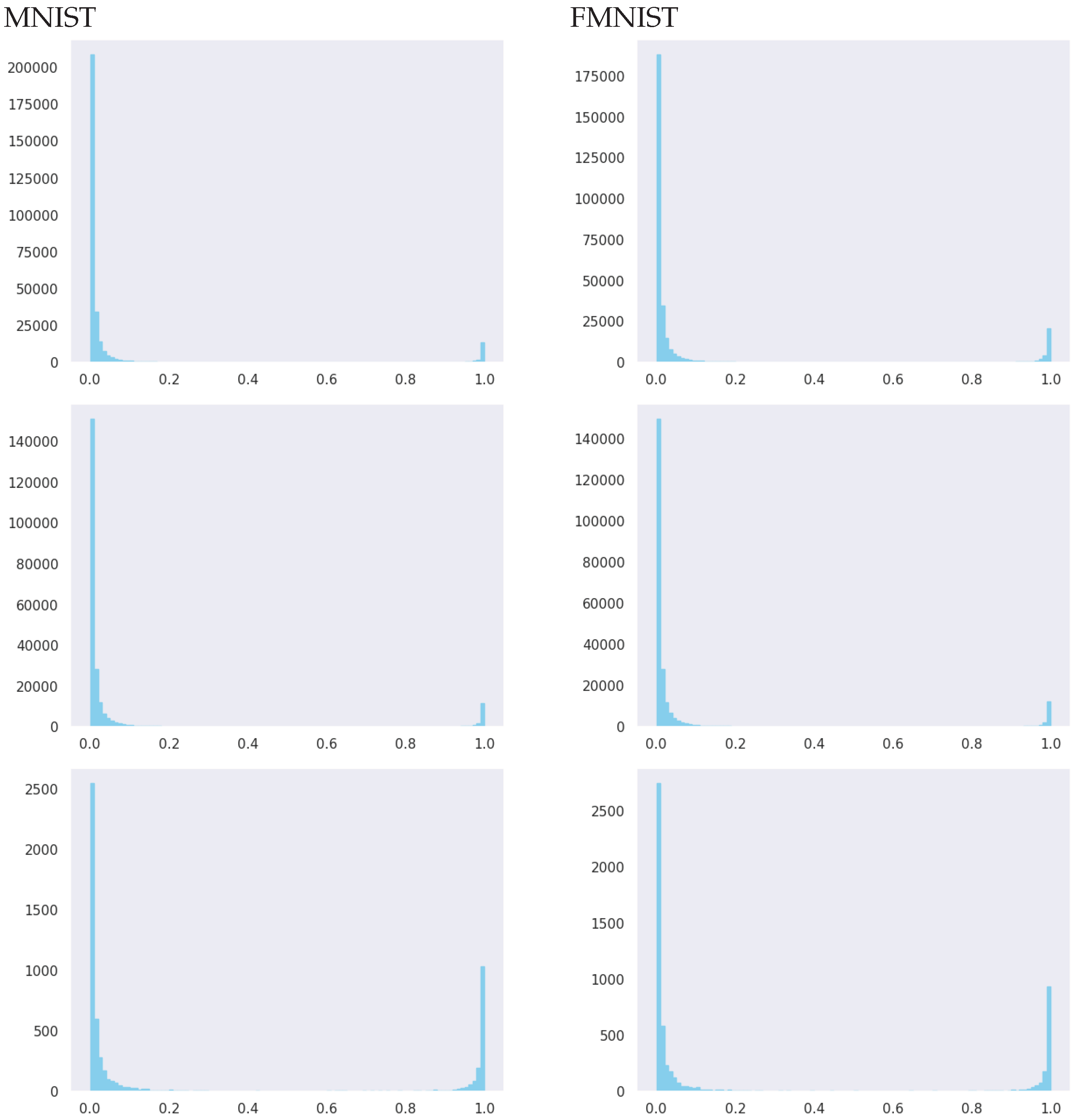
for different approaches. To guarantee reproducibility, summaries (medians, minimums, maximums) across 10 independent runs of the described experiment $s\in \{1,\dots ,10\}$ were computed for all of these statistics. Estimates of the marginal inclusion probabilities $\widehat{p}({\gamma }_{kj}^{\left(l\right)}=1|\mathcal{D})$ based on the suggested variational approximations were also computed for all of the weights. To compress the presentation of the results, we only present the mean marginal inclusion probabilities for each layer l as $\rho \left({\gamma }^{\left(l\right)}\right|\mathcal{D}):=\frac{1}{p^{(l+1)}{p}^{\left(l\right)}}{\sum }_{kj}\widehat{p}({\gamma }_{kj}^{\left(l\right)}=1|\mathcal{D})$, summarized in

Table 5. Medians and standard deviations of the average (per layer) marginal inclusion probability (see the text for the definition) for our model for MNIST, FMNIST and PHONEMNE data across 10 repeated experiments. For further details, an example of a specific distribution within a trained LBBNN-SSP-MF is shown in Figure A1.

	MNIST Data	FMNIST Data	PHONEME Data
LBBNN-SSP-MF
$\rho ({\gamma }^{\left(1\right)}=1|\mathcal{D})$	0.0844 (0.0835,0.0853)	0.1323 (0.1291,0.1349)	0.3806 (0.3764,0.3838)
$\rho ({\gamma }^{\left(2\right)}=1|\mathcal{D})$	0.0959 (0.0942,0.0967)	0.1005 (0.0981,0.1020)	0.3670 (0.3641,0.3699)
$\rho ({\gamma }^{\left(3\right)}=1|\mathcal{D})$	0.2945 (0.2808,0.3056)	0.2790 (0.2709,0.2921)	0.4236 (0.4053,0.4367)
LBBNN-SSP-MVN
$\rho ({\gamma }^{\left(1\right)}=1|\mathcal{D})$	0.2975 (0.2928,0.2993)	0.2461 (0.2410,0.2515)	0.3201 (0.3142,0.3273)
$\rho ({\gamma }^{\left(2\right)}=1|\mathcal{D})$	0.0368 (0.0363,0.0377)	0.0392 (0.0383,0.0398)	0.2287 (0.2235,0.2355)
$\rho ({\gamma }^{\left(3\right)}=1|\mathcal{D})$	0.1394 (0.1311,0.1475)	0.1462 (0.1368,0.1521)	0.2763 (0.2632,0.2953)
LBBNN-SSP-LFMVN
$\rho ({\gamma }^{\left(1\right)}=1|\mathcal{D})$	0.4474 (0.4448,0.4498)	0.4589 (0.4565,0.4603)	0.4973 (0.4965,0.4987)
$\rho ({\gamma }^{\left(2\right)}=1|\mathcal{D})$	0.4525 (0.4501,0.4537)	0.4516 (0.4493,0.4528)	0.4972 (0.4952,0.4990)
$\rho ({\gamma }^{\left(3\right)}=1|\mathcal{D})$	0.4815 (0.4685,0.4871)	0.4805 (0.4654,0.4868)	0.4979 (0.4925,0.5048)

, but we also report non-aggregated histograms in Figure A1 in the Appendix A. Last but not least, to make the abbreviations used in the reported results clear, we provide a table with their short summaries in the Abbreviations section of the paper.

4.1.1. MNIST

The results reported in Table 2 and Table 5 (with some additional results on LBBNN-SSP-LFMVN, FNN and post-training reported, respectively, in

Table A2. Performance metrics for the MNIST data, in addition to Table 2 using low factor MVN.

Prediction		Model-Prior-Method	R	All cl Acc	0.95 Threshold		Dens. Level	Epo. Time
$\mathcal{M}$	$\mathsf{\beta }$				Acc	Num.cl
SIM	SIM	LBBNN-SSP-LFMVN	1	0.959 (0.956,0.960)	-	-	0.450	13.009
SIM	SIM		10	0.979 (0.978,0.980)	1.000	7760	1.000	13.009
ALL	EXP		1	0.976 (0.976,0.978)	-	-	1.000	13.009
MED	SIM		1	0.959 (0.956,0.960)	-	-	0.449	13.009
MED	SIM		10	0.979 (0.978,0.980)	1.000	7764	0.449	13.009
MED	EXP		1	0.975 (0.974,0.977)	-	-	0.449	13.009

,

Table A5. Performance metrics of frequentist neural network under various degrees of pruning for the MNIST data.

Dens. Level	All cl Acc—Neuron Pruning	All cl Acc—Weight Pruning	Epo. Time
1.000	98.110 (98.040,98.350)	98.110 (98.040,98.350)	1.360
0.500	98.030 (97.720,98.080)	87.170 (78.260,90.730)	1.360
0.226	96.600 (95.570,97.150)	36.915 (32.600,46.910)	1.360
0.194	96.130 (94.680,96.670)	32.320 (27.320,38.150)	1.360
0.180	95.710 (93.290,96.730)	31.685 (25.010,35.840)	1.360
0.163	95.070 (91.040,96.170)	29.760 (23.810,33.340)	1.360
0.090	80.050 (75.060,90.120)	18.235 (14.500,21.520)	1.360
0.079	77.730 (68.910,86.090)	19.055 (15.270,25.990)	1.360

and

Table A8. Performance metrics for the MNIST data for the compared approaches. The results after post-training are reported here.

$\mathcal{M}$	$\mathit{\beta }$	Method	R	All cl Acc	0.95 Threshold		Density Level
					Acc	Num.cl
SIM	SIM	LBBNN-SSP-MF	1	0.967 (0.966,0.969)	-	-	0.090
SIM	SIM		10	0.980 (0.979,0.982)	0.999	8346	1.000
ALL	EXP		1	0.982 (0.980,0.983)	-	-	1.000
MED	SIM		1	0.969 (0.966,0.972)	-	-	0.079
MED	SIM		10	0.980 (0.979,0.982)	0.999	8472	0.079
MED	EXP		1	0.981 (0.980,0.984)	-	-	0.079
SIM	SIM	LBBNN-SSP-MVN	1	0.967 (0.965,0.970)	-	-	0.180
SIM	SIM		10	0.979 (0.977,0.981)	1.000	7994	1.000
ALL	EXP		1	0.980 (0.979,0.981)	-	-	1.000
MED	SIM		1	0.973 (0.971,0.977)	-	-	0.163
MED	SIM		10	0.978 (0.977,0.979)	1.000	8107	0.163
MED	EXP		1	0.976 (0.974,0.977)	-	-	0.163
SIM	SIM	LBBNN-SSP-LFMVN	1	0.971 (0.969,0.973)	-	-	0.450
SIM	SIM		10	0.978 (0.976,0.980)	0.999	8366	1.000
ALL	EXP		1	0.979 (0.978,0.980)	-	-	1.000
MED	SIM		1	0.973 (0.971,0.977)	-	-	0.449
MED	SIM		10	0.978 (0.977,0.979)	0.999	8645	0.449
MED	EXP		1	0.978 (0.976,0.979)	-	-	0.449
SIM	SIM	BNN-GP-CMF	1	0.982 (0.894,0.984)	-	-	0.226
SIM	SIM		10	0.984 (0.896,0.986)	0.995	9586	1.000
ALL	EXP		1	0.983 (0.894,0.984)	-	-	1.000
PRN	SIM	BNN-HP-MF	1	0.967 (0.965,0.968)	-	-	0.194
PRN	SIM		10	0.982 (0.981,0.983)	1.000	0007	0.194
PRN	EXP		1	0.966 (0.964,0.969)	-	-	0.194

in the Appendix) show that within our LBBNN approach: (a) model averaging across different BNNs ($R=10$) gives significantly higher accuracy than the accuracy of a random individual BNN from the model space ($R=1$); (b) the median probability model and posterior mean-based model also perform significantly better than a randomly sampled model. The performance of the median probability model and posterior mean-based model is, in fact, on par with full model averaging; (c) according to Table 5, for the mean-field variational distribution, the majority of the weights of the models have very low marginal inclusion probabilities for the weights at layers 1 and 2, while more weights have high marginal inclusion probabilities at layer 3 (although also a significant reduction at this layer). This resembles the structure of convolutional neural networks (CNN), where, typically, one first has a set of sparse convolutional layers, followed by a few fully connected layers. Unlike CNNs, the structure of sparsification is learned automatically within our approach: (d) for the MVN with full rank structure within variational approximation, the input layer is the most dense, followed by extreme sparsification in the second layer and a moderate sparsification at layer 3; (e) the MVN approach with a low factor parametrization of the covariance matrix (results in the Appendix) only provides very moderate sparsification not exceeding 50% of the weight parameters; (f) variations of all of the performance metrics across simulations are low, showing stable behavior across the repeated experiments; (g) inference with a doubt option gives almost perfect accuracy; however, this comes at the price of rejecting the classification of some of the items.

For other approaches, it is also the case that: (h) both using the posterior mean-based model and using sample averaging improves accuracy compared to a single sample from the parameter space; (i) variability in the estimates of the target parameters is low for the dense BNNs with Gaussian/mixture of Gaussians priors and BNN with Horseshoe priors and rather high for the Concrete dropout approach. When it comes to comparing our approach to baselines, we notice that: (j) dense approaches outperform sparse approaches in terms of the accuracy in general; (k) Concrete dropout marginally outperforms other approaches in terms of median accuracy; however, it exhibits large variance, whilst our full BNN and the compressed BNN with Horseshoe priors yield stable performance across experiments; (l) neither our approach nor baselines managed to reach state-of-the-art results in terms of hard classification accuracy of predictions [58]; (m) including a 95% threshold for making a classification results in a very low number of classified cases for the Horseshoe priors (it is extremely underconfident), the Concrete dropout approach seems to be overconfident when conducting an inference with the doubt option (resulting in lower accuracy but a larger number of decisions), and the full BN and BNN with Gaussian and mixture of Gaussian priors give less classified cases than the Concrete dropout approach but reach significantly higher accuracy; (n) this might mean that the thresholds need to be calibrated towards the specific methods; (o) our approach under the mean-field variational approximation and the full-rank MVN structure of variational approximation yields the highest sparsity of weights when using the median probability model. Also, (p) post-training (results in the Appendix) does not seem to significantly improve either the predictive quality of the models or uncertainty handling; (q) all BNN for all considered sparsity levels on a given configuration of the network depth and widths are significantly outperforming the frequentist counterpart (with the corresponding same sparsity levels) in terms of the generalization error. Finally, in terms of computational time, (r) as expected, FNNs were the fastest in terms of time per epoch, while for the Bayesian approaches, we see a strong positive correlation between the number of parameters and computational time, where BNN-GP-CMF is the fastest method and LBBNN-SSP-MVN is the slowest. All times were obtained while training our models on a GeForce RTX 2080 Ti GPU card. Having said that, it is important to notice that the speed difference between the fastest and slowest Bayesian approach is less than three times. Given the fact that the time is also influenced by the implementation of different methods and a potentially different load of the server when running the experiments, this might be considered quite a tolerable difference in practice.

4.1.2. FMNIST

The same set of approaches, model specifications and tuning parameters of the algorithms as in the MNIST example were used for this application. The results (a)–(r) for FMNIST data, based on Table 3 and Table 5, and Table A3 and

Table A9. Performance metrics for the FMNIST data for the compared approaches. The results after post-training are reported here.

$\mathcal{M}$	$\mathit{\beta }$	Method	R	All cl Acc	0.95 Threshold		Density Level
					Acc	Num.cl
SIM	SIM	LBBNN-SSP-MF	1	0.863 (0.862,0.869)	-	-	0.120
SIM	SIM		10	0.884 (0.881,0.886)	0.995	4932	1.000
ALL	EXP		1	0.882 (0.879,0.887)	-	-	1.000
MED	SIM		1	0.866 (0.865,0.869)	-	-	0.108
MED	SIM		10	0.885 (0.882,0.887)	0.995	4994	0.108
MED	EXP		1	0.882 (0.878,0.886)	-	-	0.108
SIM	SIM	LBBNN-SSP-MVN	1	0.859 (0.857,0.862)	-	-	0.156
SIM	SIM		10	0.880 (0.874,0.881)	0.996	4615	1.000
ALL	EXP		1	0.876 (0.872,0.877)	-	-	1.000
MED	SIM		1	0.863 (0.860,0.865)	-	-	0.129
MED	SIM		10	0.878 (0.874,0.880)	0.995	4801	0.129
MED	EXP		1	0.873 (0.870,0.875)	-	-	0.129
SIM	SIM	LBBNN-SSP-LFMVN	1	0.847 (0.844,0.850)	-	-	0.456
SIM	SIM		10	0.875 (0.873,0.878)	0.996	4431	1.000
ALL	EXP		1	0.866 (0.859,0.868)	-	-	1.000
MED	SIM		1	0.846 (0.844,0.849)	-	-	0.455
MED	SIM		10	0.876 (0.873,0.879)	0.996	4426	0.455
MED	EXP		1	0.864 (0.860,0.865)	-	-	0.455
SIM	SIM	BNN-GP-CMF	1	0.897 (0.820,0.899)	-	-	0.094
SIM	SIM		10	0.897 (0.823,0.902)	0.943	8826	1.000
ALL	EXP		1	0.896 (0.820,0.901)	-	-	1.000
PRN	SIM	BNN-HP-MF	1	0.867 (0.864,0.871)	-	-	0.302
PRN	SIM		10	0.888 (0.887,0.890)	1.000	0147	0.302
PRN	EXP		1	0.868 (0.864,0.869)	-	-	0.302

in Appendix A, are completely consistent with the results from the MNIST experiment; however, the predictive performances for all of the approaches are poorer on FMNIST. Also, whilst full BNN and BNN with Horseshoe priors on FMNIST obtbain lower sparsity levels than on MNIST, Concrete dropout here improves in this sense compared to the previous example. For FNN, the same conclusions as those obtained for the MNIST dataset are valid (see

Table A6. Performance metrics of frequentist neural network under various degrees of pruning for the FMNIST data.

Dens. Level	All cl Acc—Neuron Pruning	All cl Acc—Weight Pruning	Epo. Time
1.000	89.470 (86.240,89.790)	89.470 (86.240,89.790)	1.260
0.500	85.150 (80.040,87.180)	29.865 (21.370,41.080)	1.260
0.302	67.610 (53.110,75.760)	17.175 (14.020,20.660)	1.260
0.156	41.595 (37.520,45.510)	11.460 (9.370,20.720)	1.260
0.129	39.040 (30.090,44.980)	10.515 (9.300,18.490)	1.260
0.120	39.775 (26.140,44.480)	09.980 (8.130,18.610)	1.260
0.108	38.750 (23.890,43.660)	10.325 (8.080,20.110)	1.260
0.094	36.340 (23.640,41.050)	09.790 (8.040,25.000)	1.260

for details).

4.1.3. PHONEME

Finally, the same set of approaches, model specifications (except for having 256 input covariates and 5 classes of the responses) and tuning parameters of the algorithms as in the MNIST and FMNIST examples were used for the classification of PHONEME data. The results (a)–(r) for the PHONEME data, based on Table 4 and Table 5, and

Table A4. Performance metrics for the PHONEME data, in addition to Table 4 using low factor MVN.

Prediction		Model-Prior-Method	R	All cl Acc	0.95 Threshold		Dens. Level	Epo. Time
$\mathcal{M}$	$\mathsf{\beta }$				Acc	Num.cl
SIM	SIM	LBBNN-SSP-LFMVN	1	0.918 (0.906,0.928)	-	-	0.497	0.472
SIM	SIM		10	0.929 (0.926,0.934)	0.994	663	1.000	0.472
ALL	EXP		1	0.921 (0.915,0.931)	-	-	1.000	0.472
MED	SIM		1	0.918 (0.909,0.930)	-	-	0.497	0.472
MED	SIM		10	0.929 (0.925,0.933)	0.995	664	0.497	0.472
MED	EXP		1	0.917 (0.912,0.925)	-	-	0.497	0.472

and

Table A10. Performance metrics for the PHONEME data for the compared approaches. The results after post-training are reported here.

$\mathcal{M}$	$\mathit{\beta }$	Method	R	All cl Acc	0.95 Threshold		Density Level
					Acc	Num.cl
SIM	SIM	LBBNN-SSP-MF	1	0.917 (0.895,0.928)	-	-	0.120
SIM	SIM		10	0.927 (0.921,0.931)	0.991	703	1.000
ALL	EXP		1	0.924 (0.923,0.929)	-	-	1.000
MED	SIM		1	0.924 (0.910,0.930)	-	-	0.108
MED	SIM		10	0.924 (0.911,0.932)	0.981	772	0.108
MED	EXP		1	0.925 (0.909,0.931)	-	-	0.108
SIM	SIM	LBBNN-SSP-MVN	1	0.922 (0.914,0.928)	-	-	0.255
SIM	SIM		10	0.931 (0.926,0.935)	0.993	682	1.000
ALL	EXP		1	0.927 (0.917,0.932)	-	-	1.000
MED	SIM		1	0.923 (0.919,0.931)	-	-	0.225
MED	SIM		10	0.928 (0.924,0.933)	0.991	691	0.225
MED	EXP		1	0.924 (0.915,0.930)	-	-	0.225
SIM	SIM	LBBNN-SSP-LFMVN	1	0.919 (0.910,0.926)	-	-	0.497
SIM	SIM		10	0.929 (0.925,0.931)	0.994	678	1.000
ALL	EXP		1	0.921 (0.912,0.933)	-	-	1.000
MED	SIM		1	0.917 (0.895,0.926)	-	-	0.497
MED	SIM		10	0.928 (0.923,0.932)	0.994	676	0.497
MED	EXP		1	0.917 (0.909,0.926)	-	-	0.497
SIM	SIM	BNN-GP-CMF	1	0.882 (0.716,0.904)	-	-	0.509
SIM	SIM		10	0.921 (0.918,0.930)	0.960	189	1.000
ALL	EXP		1	0.877 (0.697,0.909)	-	-	1.000
PRN	SIM	BNN-HP-MF	1	0.913 (0.909,0.926)	-	-	0.457
PRN	SIM		10	0.917 (0.916,0.922)	0.936	037	0.457
PRN	EXP		1	0.917 (0.914,0.924)	-	-	0.457

in Appendix A, are also overall consistent with the results from the MNIST and FMNIST experiments; however, predictive performances for all of the approaches are better than on FMNIST yet worse than on MNIST. All of the methods, where sparsifications are possible, gave a lower sparsity level for this example.

Yet, rather considerable sparsification is still shown to be feasible. For FNN, the same conclusions as those obtained for MNIST and FMNIST datasets are valid, though the deterioration of performance of FNN here was less drastic (see

Table A7. Performance metrics of frequentist neural network under various degrees of pruning for the PHONEMNE data.

Dens. Level	All cl Acc—Neuron Pruning	All cl Acc—Weight Pruning	Epo. Time
1.000	92.400 (92.1,92.9)	92.500 (92.200,92.700)	0.029
0.600	92.250 (91.8,93.2)	88.050 (86.100,90.500)	0.029
0.509	92.100 (91.5,92.7)	82.650 (78.100,85.400)	0.029
0.457	92.100 (91.6,92.7)	80.950 (75.700,86.500)	0.029
0.371	91.850 (90.4,92.6)	76.050 (68.300,82.200)	0.029
0.307	91.700 (90.7,92.3)	71.950 (66.500,80.200)	0.029
0.255	91.000 (90.4,92.8)	67.900 (58.600,80.200)	0.029
0.225	90.700 (90.2,92.6)	64.950 (51.800,77.300)	0.029

for details).

5. Discussion

In this paper, we have introduced the concept of Bayesian model (or structural) uncertainty in BNNs and suggested a scalable variational inference technique for approximating the joint posterior of models and the parameters of these models. Approximate posterior predictive distributions, with both models and parameters marginalized out, can be easily obtained. Furthermore, marginal inclusion probabilities give proper probabilistic interpretation to Bayesian binary dropout and allow for the performance of model (or architecture) selection. The latter allows for solving the overparametrization issue present in BNNs and can lead to more interpretable deep learning models in the future.

We provide image, sound and tabular dataset classification applications of the suggested technique, showing that it both allows for significantly sparsifying neural networks without a noticeable loss of predictive power and accurately handles the predictive uncertainty.

Regarding the computational costs of optimization, in stochastic variational inference, the iteration cost consists of a product of the number of data points in a sample times the number of parameters in the variational distribution times the number of samples from the model. In our case, for the mean-field approximations, we are introducing only one additional parameter ${\alpha }_{kj}^{\left(l\right)}$ for each weight. With underlying Gaussian structure on ${\mathsf{\alpha }}^{\left(l\right)}$, however, additional parameters of the covariance matrix are further introduced. The complexity of each optimization step is proportional to the number of parameters to optimize; thus, the deterioration in terms of computational time (as demonstrated in the experiments) is, although present, not at all drastic as compared to the fully connected BNN. For the FNN, however, we do not sample the parameters in each iteration to approximate the gradient; thus, the computations become further cheaper by a factor corresponding to the number of samples one addresses in BNNs. Yet, as demonstrated in the experiments of this paper, the deterioration of the training costs of BNNs is not that drastic as compared to FNNs (Table A5, Table A6 and Table A7). Furthermore, the complexities of different methods are proportional to the number of “active” parameters involved in predictions, typically giving benefits to more sparse methods, which we obtain through model selection. See

Table 6. Comparison of computational complexities for the model training step and prediction step in this paper for the proposed methods and the baselines, assuming first-order stochastic optimization is used, where N is the subsample size for training, $\left|\mathsf{\beta }\right|$ is the cardinality of the set of weights in the full architecture with layers of weights, M is the number of samples from the model per iteration of optimization, R is the number of samples from the model per prediction and $\tilde{S}$ is the density level at the prediction step. Note that multipliers for $\left|\mathsf{\beta }\right|$ are added for comparison reasons within similar complexities.

Method	Training	Prediction per Data Point
FNN	$O(N\times |\mathsf{\beta }\left|\right)$	$O\left(\right|\mathsf{\beta }\left|\right)$
BNN-GP-MF	$O(N\times M\times 2|\mathsf{\beta }\left|\right)$	$O(R\times 2|\mathsf{\beta }\left|\right)$
BNN-MGP-MF	$O(N\times M\times 2|\mathsf{\beta }\left|\right)$	$O(R\times 2|\mathsf{\beta }\left|\right)$
BNN-GP-CMF	$O(N\times M\times 2|\mathsf{\beta }\left|\right)$	$O(R\times 2|\mathsf{\beta }\left|\right)$
BNN-HP-MF	$O(N\times M\times 3|\mathsf{\beta }\left|\right)$	$O(R\times 3|\mathsf{\beta }|\times \tilde{S})$
LBBNN-SSP-MF	$O(N\times M\times 3|\mathsf{\beta }\left|\right)$	$O(R\times 3|\mathsf{\beta }|\times \tilde{S})$
LBBNN-SSP-MVN	$O(N\times M\times |\mathsf{\beta }{|}^2)$	$O(R\times |\mathsf{\beta }{|}^2\times \tilde{S})$
LBBNN-SSP-LFMVN	$O(N\times M\times 5|\mathsf{\beta }\left|\right)$	$O(R\times 5|\mathsf{\beta }|\times \tilde{S})$

for more details.

Regarding practical recommendations, we suggest, based on our empirical results, using LBBNN-SSP-MF if one is interested in a reasonable trade-off between sparsity, predictive accuracy and uncertainty. One should make model averaging across several samples to increase the accuracy of the predictions or use the posterior mean-based model. One sample is typically not enough to have sufficient accuracy. For sparsification, the use of the median probability model is advised. Also, if a doubt decision is allowed for uncertain cases, one is expected to obtain almost perfect accuracy for the rest of the predictions. LBBNN-SSP-MVN and LBBNN-SSP-LFMVN are computationally more costly than LBBNN-SSP-MF and do not provide superior performance concerning the latter; thus, these two modifications are not recommended. If sparsity is not needed, standard BNN-GP-MF and BNN-MGP-MF are sufficient.

Currently, fairly simple prior distributions for both models and parameters are used. These prior distributions are assumed independent across the parameters of the neural network, which might not always be reasonable. Alternatively, both parameter and model priors can incorporate joint-dependent structures, which can further improve the sparsification of the configurations of neural networks. When it comes to the model priors with local structures and dependencies between the variables (neurons), one can mention the so-called dilution priors [59]. These priors take care of the similarities between models by down-weighting the probabilities of the models with highly correlated variables. There are also numerous approaches to incorporate interdependencies between the model parameters via priors in different settings within simpler models [60,61,62]. Obviously, in the context of inference in the joint parameter-model settings in BNNs, more research should be conducted on the choice of priors.

The main limitation of the article is the absence of a theoretical guarantee of selecting the true data-generative process under the combination of the addressed priors for BNNs. Also, the suggested methodology results in increased computational costs compared to the simpler BNNs and FNNs. Last but not least, the nature of that variational Bayes in an approximate technique is a limitation in itself, and we could not compare it to the ground truth under model and parameter uncertainty in BNNs, that is, to be obtained by exact MCMC sampling due to the fact that the latter is not feasible in the addressed high-dimensional settings. Theoretical guarantees on the convergence of the approximate variational inference procedure to the true target are also problematic under practical regularity conditions, which is a considerable limitation. Lastly, due to the computational challenges, only relatively small networks have been considered in this work. Evaluation of the methods on larger networks with billions of parameters is certainly of interest and should be conducted with further developments in computational technologies.

In this work, we restrict ourselves to a subclass of BNNs, defined by the inclusion–exclusion of particular weights within a given architecture. In the future, it can be of particular interest to extend the approach to the choice of the activation functions as well as the maximal depth and width of each layer of the BNN. This can be performed by a combination of a set of different activation functions for neurons within a layer on one hand and allowing skip connections from every layer to the response on the other hand. A more detailed discussion of these possibilities and ways to proceed is given in Hubin [41]. Finally, theoretical and empirical studies of the accuracy of variational inference within these complex nonlinear models should be performed. Even within linear models, Carbonetto et al. [44] have shown that the results can be strongly biased. Various approaches for reducing the bias in variational inference are developed. One can either use more flexible families of variational distributions by, for example, introducing auxiliary variables [63,64], normalizing flows [65], diffusion-based variational distributions [66] or addressing Jackknife to remove the bias [67]. We leave these opportunities for further research.

References

1. Goodfellow, I.; Bengio, Y.; Courville, A. Deep Learning; MIT Press: Cambridge, MA, USA, 2016; Available online: http://www.deeplearningbook.org (accessed on 25 January 2024).
2. Refenes, A.N.; Zapranis, A.; Francis, G. Stock performance modeling using neural networks: A comparative study with regression models. Neural Netw. 1994, 7, 375–388. [Google Scholar] [CrossRef]
3. Razi, M.A.; Athappilly, K. A comparative predictive analysis of neural networks (NNs), nonlinear regression and classification and regression tree (CART) models. Expert Syst. Appl. 2005, 29, 65–74. [Google Scholar] [CrossRef]
4. Adya, M.; Collopy, F. How effective are neural networks at forecasting and prediction? A review and evaluation. J. Forecast. 1998, 17, 481–495. [Google Scholar] [CrossRef]
5. Sargent, D.J. Comparison of artificial neural networks with other statistical approaches. Cancer 2001, 91, 1636–1642. [Google Scholar] [CrossRef]
6. Kanter, J.M.; Veeramachaneni, K. Deep feature synthesis: Towards automating data science endeavors. In Proceedings of the IEEE International Conference on Data Science and Advanced Analytics (DSAA), Paris, France, 19–21 October 2015; pp. 1–10. [Google Scholar]
7. Gawlikowski, J.; Tassi, C.R.N.; Ali, M.; Lee, J.; Humt, M.; Feng, J.; Kruspe, A.; Triebel, R.; Jung, P.; Roscher, R.; et al. A survey of uncertainty in deep neural networks. arXiv 2021, arXiv:2107.03342. [Google Scholar] [CrossRef]
8. Neklyudov, K.; Molchanov, D.; Ashukha, A.; Vetrov, D. Variance Networks: When Expectation Does Not Meet Your Expectations. In Proceedings of the International Conference on Learning Representations, Vancouver, BC, Canada, 30 April–3 May 2018. [Google Scholar]
9. Raftery, A.E.; Madigan, D.; Hoeting, J.A. Bayesian Model Averaging for Linear Regression Models. J. Am. Stat. Assoc. 1997, 92, 179–191. [Google Scholar] [CrossRef]
10. Polson, N.G.; Ročková, V. Posterior concentration for sparse deep learning. In Proceedings of the Advances in Neural Information Processing Systems 31: Annual Conference on Neural Information Processing Systems 2018, NeurIPS 2018, Montréal, QC, Canada, 3–8 December 2018. [Google Scholar]
11. Hubin, A.; Storvik, G. Combining model and parameter uncertainty in Bayesian neural networks. arXiv 2019, arXiv:1903.07594. [Google Scholar]
12. Bai, J.; Song, Q.; Cheng, G. Efficient variational inference for sparse deep learning with theoretical guarantee. In Proceedings of the Advances in Neural Information Processing Systems 33: Annual Conference on Neural Information Processing Systems 2020, NeurIPS 2020, virtual, 6–12 December 2020; pp. 466–476. [Google Scholar]
13. Papamarkou, T.; Skoularidou, M.; Palla, K.; Aitchison, L.; Arbel, J.; Dunson, D.; Filippone, M.; Fortuin, V.; Hennig, P.; Hubin, A.; et al. Position Paper: Bayesian Deep Learning in the Age of Large-Scale AI. arXiv 2024, arXiv:2402.00809. [Google Scholar]
14. Breiman, L. The little bootstrap and other methods for dimensionality selection in regression: X-fixed prediction error. J. Am. Stat. Assoc. 1992, 87, 738–754. [Google Scholar] [CrossRef]
15. Jylänki, P.; Nummenmaa, A.; Vehtari, A. Expectation Propagation for Neural Networks with Sparsity-Promoting Priors. J. Mach. Learn. Res. 2014, 15, 1849–1901. [Google Scholar]
16. Blundell, C.; Cornebise, J.; Kavukcuoglu, K.; Wierstra, D. Weight uncertainty in neural network. In Proceedings of the International Conference on Machine Learning, Lille, France, 6–11 July 2015; pp. 1613–1622. [Google Scholar]
17. Overweg, H.; Popkes, A.L.; Ercole, A.; Li, Y.; Hernández-Lobato, J.M.; Zaykov, Y.; Zhang, C. Interpretable outcome prediction with sparse Bayesian neural networks in intensive care. arXiv 2019, arXiv:1905.02599. [Google Scholar]
18. Molchanov, D.; Ashukha, A.; Vetrov, D. Variational dropout sparsifies deep neural networks. In Proceedings of the International Conference on Machine Learning, Sydney, Australia, 6–11 August 2017; pp. 2498–2507. [Google Scholar]
19. Ghosh, S.; Yao, J.; Doshi-Velez, F. Structured variational learning of Bayesian neural networks with horseshoe priors. In Proceedings of the International Conference on Machine Learning, Stockholm, Sweden, 10–15 July 2018; pp. 1744–1753. [Google Scholar]
20. Neklyudov, K.; Molchanov, D.; Ashukha, A.; Vetrov, D.P. Structured bayesian pruning via log-normal multiplicative noise. In Proceedings of the Advances in Neural Information Processing Systems 30: Annual Conference on Neural Information Processing Systems 2017, Long Beach, CA, USA, 4–9 December 2017; pp. 6775–6784. [Google Scholar]
21. Ghosh, S.; Yao, J.; Doshi-Velez, F. Model Selection in Bayesian Neural Networks via Horseshoe Priors. J. Mach. Learn. Res. 2019, 20, 1–46. [Google Scholar]
22. Louizos, C.; Ullrich, K.; Welling, M. Bayesian compression for deep learning. In Proceedings of the Advances in Neural Information Processing Systems 30: Annual Conference on Neural Information Processing Systems 2017, Long Beach, CA, USA, 4–9 December 2017; pp. 3288–3298. [Google Scholar]
23. Carvalho, C.M.; Polson, N.G.; Scott, J.G. Handling sparsity via the horseshoe. In Proceedings of the Artificial Intelligence and Statistics, Clearwater Beach, FL, USA, 16–18 April 2009; pp. 73–80. [Google Scholar]
24. Bardenet, R.; Doucet, A.; Holmes, C. Towards scaling up Markov chain Monte Carlo: An adaptive subsampling approach. In Proceedings of the International Conference on Machine Learning, Beijing, China, 21–26 June 2014; pp. 405–413. [Google Scholar]
25. Bardenet, R.; Doucet, A.; Holmes, C. On Markov chain Monte Carlo methods for tall data. J. Mach. Learn. Res. 2017, 18, 1515–1557. [Google Scholar]
26. Korattikara, A.; Chen, Y.; Welling, M. Austerity in MCMC land: Cutting the Metropolis-Hastings budget. In Proceedings of the International Conference on Machine Learning, Beijing, China, 21–26 June 2014; pp. 181–189. [Google Scholar]
27. Quiroz, M.; Kohn, R.; Villani, M.; Tran, M.N. Speeding up MCMC by efficient data subsampling. J. Am. Stat. Assoc. 2018, 114, 831–843. [Google Scholar] [CrossRef]
28. Welling, M.; Teh, Y.W. Bayesian learning via stochastic gradient Langevin dynamics. In Proceedings of the 28th International Conference on Machine Learning (ICML-11), Bellevue, WA, USA, 28 June–2 July 2011; pp. 681–688. [Google Scholar]
29. Quiroz, M.; Villani, M.; Kohn, R. Exact subsampling MCMC. arXiv 2016, arXiv:1603.08232. [Google Scholar] [CrossRef]
30. Maclaurin, D.; Adams, R.P. Firefly Monte Carlo: Exact MCMC with Subsets of Data. In Proceedings of the Conference on Uncertainty in Artificial Intelligence, Quebec City, QC, Canada, 23–27 July 2014; pp. 543–552. [Google Scholar]
31. Liu, S.; Mingas, G.; Bouganis, C.S. An exact MCMC accelerator under custom precision regimes. In Proceedings of the 2015 International Conference on Field Programmable Technology (FPT), Queenstown, New Zealand, 7–9 December 2015; pp. 120–127. [Google Scholar]
32. Jordan, M.I.; Ghahramani, Z.; Jaakkola, T.S.; Saul, L.K. An introduction to variational methods for graphical models. Mach. Learn. 1999, 37, 183–233. [Google Scholar] [CrossRef]
33. Ahmed, A.; Aly, M.; Gonzalez, J.; Narayanamurthy, S.; Smola, A.J. Scalable inference in latent variable models. In Proceedings of the Fifth ACM International Conference on Web Search and Data Mining, Seattle, WA, USA, 8–12 February 2012; pp. 123–132. [Google Scholar]
34. Humphreys, K.; Titterington, D. Approximate Bayesian inference for simple mixtures. In Proceedings of the COMPSTAT: Proceedings in Computational Statistics 14th Symposium, Utrecht, The Netherlands, 21–25 August 2000; pp. 331–336. [Google Scholar]
35. Foti, N.; Xu, J.; Laird, D.; Fox, E. Stochastic variational inference for hidden Markov models. In Proceedings of the Advances in Neural Information Processing Systems 27: Annual Conference on Neural Information Processing Systems 2014, Montreal, QC, Canada, 8–13 December 2014; Volume 27. [Google Scholar]
36. Attias, H. A variational Baysian framework for graphical models. In Proceedings of the Advances in Neural Information Processing Systems 12, NIPS Conference, Denver, CO, USA, 29 November–4 December 1999; pp. 209–215. [Google Scholar]
37. Graves, A. Practical variational inference for neural networks. In Proceedings of the Advances in Neural Information Processing Systems 24: 25th Annual Conference on Neural Information Processing Systems 2011, Granada, Spain, 12–14 December 2011; pp. 2348–2356. [Google Scholar]
38. Gal, Y. Uncertainty in Deep Learning. PhD Thesis, University of Cambridge, Cambridge, UK, 2016. [Google Scholar]
39. Sun, Y.; Song, Q.; Liang, F. Learning sparse deep neural networks with a spike-and-slab prior. Stat. Probab. Lett. 2022, 180, 109246. [Google Scholar] [CrossRef]
40. Bhattacharya, S.; Liu, Z.; Maiti, T. Comprehensive study of variational Bayes classification for dense deep neural networks. Stat. Comput. 2024, 34, 17. [Google Scholar] [CrossRef]
41. Hubin, A. Bayesian model configuration, selection and averaging in complex regression contexts. PhD Thesis, University of Oslo, Oslo, Norway, 2018. [Google Scholar]
42. Clyde, M.A.; Ghosh, J.; Littman, M.L. Bayesian Adaptive Sampling for Variable Selection and Model Averaging. J. Comput. Graph. Stat. 2011, 20, 80–101. [Google Scholar] [CrossRef]
43. Logsdon, B.A.; Hoffman, G.E.; Mezey, J.G. A variational Bayes algorithm for fast and accurate multiple locus genome-wide association analysis. BMC Bioinform. 2010, 11, 58. [Google Scholar] [CrossRef]
44. Carbonetto, P.; Stephens, M. Scalable variational inference for Bayesian variable selection in regression, and its accuracy in genetic association studies. Bayesian Anal. 2012, 7, 73–108. [Google Scholar] [CrossRef]
45. Srivastava, N.; Hinton, G.; Krizhevsky, A.; Sutskever, I.; Salakhutdinov, R. Dropout: A simple way to prevent neural networks from overfitting. J. Mach. Learn. Res. 2014, 15, 1929–1958. [Google Scholar]
46. Kingma, D.P.; Salimans, T.; Welling, M. Variational dropout and the local reparameterization trick. In Proceedings of the Advances in Neural Information Processing Systems 28: Annual Conference on Neural Information Processing Systems 2015, Montreal, QC, Canada, 7–12 December 2015; pp. 2575–2583. [Google Scholar]
47. Gal, Y.; Hron, J.; Kendall, A. Concrete dropout. In Proceedings of the Advances in Neural Information Processing Systems 30: Annual Conference on Neural Information Processing Systems 2017, Long Beach, CA, USA, 4–9 December 2017; pp. 3581–3590. [Google Scholar]
48. Wasserman, L. Bayesian model selection and model averaging. J. Math. Psychol. 2000, 44, 92–107. [Google Scholar] [CrossRef] [PubMed]
49. Barbieri, M.M.; Berger, J.O. Optimal predictive model selection. Ann. Stat. 2004, 32, 870–897. [Google Scholar] [CrossRef]
50. Hernández-Lobato, J.M.; Hernández-Lobato, D.; Suárez, A. Expectation propagation in linear regression models with spike-and-slab priors. Mach. Learn. 2015, 99, 437–487. [Google Scholar] [CrossRef]
51. LeCun, Y.; Cortes, C.; Burges, C. MNIST Handwritten Digit Database. 1998. Available online: http://yann.lecun.com/exdb/mnist/ (accessed on 25 January 2024).
52. Xiao, H.; Rasul, K.; Vollgraf, R. Fashion-MNIST: A novel image dataset for benchmarking machine learning algorithms. arXiv 2017, arXiv:1708.07747. [Google Scholar]
53. Hastie, T.; Buja, A.; Tibshirani, R. Penalized discriminant analysis. Ann. Stat. 1995, 23, 73–102. [Google Scholar] [CrossRef]
54. Kingma, D.P.; Ba, J. Adam: A method for stochastic optimization. arXiv 2014, arXiv:1412.6980. [Google Scholar]
55. Blalock, D.; Gonzalez Ortiz, J.J.; Frankle, J.; Guttag, J. What is the state of neural network pruning? Proc. Mach. Learn. Syst. 2020, 2, 129–146. [Google Scholar]
56. Posch, K.; Steinbrener, J.; Pilz, J. Variational Inference to Measure Model Uncertainty in Deep Neural Networks. arXiv 2019, arXiv:1902.10189. [Google Scholar]
57. Ripley, B.D. Pattern Recognition and Neural Networks; Cambridge University Press: Cambridge, UK, 2007. [Google Scholar]
58. Palvanov, A.; Im Cho, Y. Comparisons of deep learning algorithms for MNIST in real-time environment. Int. J. Fuzzy Log. Intell. Syst. 2018, 18, 126–134. [Google Scholar] [CrossRef]
59. George, E.I. Dilution priors: Compensating for model space redundancy. In Borrowing Strength: Theory Powering Applications–A Festschrift for Lawrence D. Brown; Institute of Mathematical Statistics: Houston, TX, USA, 2010; pp. 158–165. [Google Scholar]
60. Smith, T.E.; LeSage, J.P. A Bayesian probit model with spatial dependencies. In Spatial and Spatiotemporal Econometrics; Emerald Group Publishing Limited: Bingley, UK, 2004; pp. 127–160. [Google Scholar]
61. Fahrmeir, L.; Lang, S. Bayesian inference for generalized additive mixed models based on Markov random field priors. J. R. Stat. Soc. Ser. C (Appl. Stat.) 2001, 50, 201–220. [Google Scholar] [CrossRef]
62. Dobra, A.; Hans, C.; Jones, B.; Nevins, J.R.; Yao, G.; West, M. Sparse graphical models for exploring gene expression data. J. Multivar. Anal. 2004, 90, 196–212. [Google Scholar] [CrossRef]
63. Ranganath, R.; Tran, D.; Blei, D. Hierarchical variational models. In Proceedings of the International Conference on Machine Learning, New York, NY, USA, 19–24 June 2016; pp. 324–333. [Google Scholar]
64. Salimans, T.; Kingma, D.; Welling, M. Markov chain Monte Carlo and variational inference: Bridging the gap. In Proceedings of the International Conference on Machine Learning, Lille, France, 6–11 July 2015; pp. 1218–1226. [Google Scholar]
65. Louizos, C.; Welling, M. Multiplicative normalizing flows for variational Bayesian neural networks. In Proceedings of the International Conference on Machine Learning, Sydney, Australia, 6–11 August 2017; pp. 2218–2227. [Google Scholar]
66. Kingma, D.; Salimans, T.; Poole, B.; Ho, J. Variational diffusion models. In Proceedings of the Advances in Neural Information Processing Systems 34: Annual Conference on Neural Information Processing Systems 2021, NeurIPS 2021, virtual, 6–14 December 2021; pp. 21696–21707. [Google Scholar]
67. Nowozin, S. Debiasing evidence approximations: On importance-weighted autoencoders and jackknife variational inference. In Proceedings of the International Conference on Learning Representations, Vancouver, BC, Canada, 30 April–3 May 2018. [Google Scholar]
68. UCI. Dry Bean Dataset. UCI Machine Learning Repository. 2020. Available online: https://archive.ics.uci.edu/dataset/602/dry+bean+dataset (accessed on 25 January 2024).
69. Quinlan, Q. Credit Approval. UCI Machine Learning Repository. 2007. Available online: https://archive.ics.uci.edu/dataset/27/credit+approval (accessed on 25 January 2024).
70. Moro, S.; Rita, P.; Cortez, P. Bank Marketing. UCI Machine Learning Repository. 2012. Available online: https://archive.ics.uci.edu/dataset/222/bank+marketing (accessed on 25 January 2024).
71. Kohavi, R. Census Income. UCI Machine Learning Repository. 1996. Available online: https://archive.ics.uci.edu/dataset/20/census+income (accessed on 25 January 2024).
72. ÇINAR, İ.; Koklu, M.; Taşdemir, Ş. Classification of raisin grains using machine vision and artificial intelligence methods. Gazi Mühendislik Bilim. Derg. 2020, 6, 200–209. [Google Scholar]
73. Ozkan, I.; Koklu, M.; Saraçoğlu, R. Classification of pistachio species using improved k-NN classifier. Health 2021, 23, e2021044. [Google Scholar]
Figure 1. Illustrations of the proposed variational families. On the left: mean field approximation. On the right: approximation with multivariate Gaussian structure for α ’s. Here, for simplicity, the indices of layers are dropped and a single index for weights is used.
Mathematics 12 00788 g001
Figure 2. Graph of relations between the compared methods.
Mathematics 12 00788 g002