1. Introduction
The initial formulation for solving problems of mathematical physics using integral equations refers to the works of Fredholm, who first proposed the study and solution of classical problems of mathematical physics using the transformation of the original differential equations to the formulation of the problem for solving related integral equations, later called Fredholm equations. The solution of problems of mathematical physics, both in the form of differential and integral equations. at that time was impossible using numerical methods and methods of discretization of the initial problem via a grid of high dimensionality in the number of elementary partitions, as such problems were associated with impossible manual calculations. With the development of computer technology appeared the formulation and the first methods and algorithms for distributed computations over differential equations, allowing the modeling of real physical processes, and integral equations were used less frequently, due to problems with the complexity of calculations, in the solution of systems of linear algebraic equations (SLEs) over fully filled operator matrices.
Mikhlin, in his works, investigated different variations of problem statements for solving integral equations in the theory of elasticity [
1], and also investigated the possibilities of obtaining analytical and numerical solutions of singular integral equations [
2,
3] related to the problems of mathematical physics. Colton and Kress considered surface and volume problems of acoustics and electrodynamics based on integral equations, as well as their numerical formulations [
4]. In these papers, however, due to the reasons described above, there were no numerical results accompanying test problems. Miller, in a series of papers [
5], also investigated modern formulations for the solution of electrodynamics problems on the basis of computational methods for solving bulk singular integral equations, using features of kernels of integral operators based on Green’s functions [
4], satisfying solutions for the volumetric Helmholtz equation.
Mathematical formulation and development of effective computational methods for solving problems of mathematical physics are the most important areas of science and technology development today. Modern problems are associated with large requirements for accuracy and speed of computation, in view of which the requirements of the dimensionality of discretization of problems increase. The classical formulation of the solution of differential and integral equations, as well as general computational methods for solution, are becoming insufficient to meet the needs of experimenters, researchers and manufacturers. This aspect pushes us to the necessity of developing effective methods for solving specific problem formulations based on a priori factual knowledge, assumptions about the structure of the solution, and constraints on the conditions at the boundary of the domain [
6].
Overcoming these limitations, recent works on computational methods, applicable to the solution of differential equations that reduce to solving systems of linear equations (SLEs) with high-dimensional sparse operator matrices, have proposed a series of approximate methods capable of addressing the problem of increasing the discretization of the solution domain, based on homotopies. Among these are the homotopy method described in detail in [
7], the multigrid method [
8], the multigrid–homotopy method [
9], and the wavelet multiscale method [
10]. These methods are traditionally used in tasks related to solving problems of mathematical physics, including, for example, [
11,
12,
13], and conducting numerical experiments with models based on partial differential equations.
Homotopy methods [
7] for approximate solutions of large-dimensional SLEs, resulting from the discretization of the solution domain of the corresponding differential equation, allow the obtaining of solutions with specified accuracy on large grids. The main idea of the method is to use the concept of homotopy for a gradual transition from a simplified version of the problem to its original, more complex form, while following a path that maintains connectivity between solutions. The homotopy grid method is especially useful in cases where direct solving of the original problem is difficult due to its complexity or the presence of multiple local minima/maxima.
The algebraic multigrid method [
8] represents a class of algorithms for solving systems of linear equations, particularly effective for large sparse matrices arising from the discretization of differential equations. This method does not require explicit knowledge of the geometry of the problem and is built directly on the basis of the equation coefficients, making it applicable to a wider class of problems. The key idea of multigrid methods is to use iterations at different levels of discretization (grids) to accelerate convergence to the solution. Simplified versions of the original problem are solved on coarse grids, effectively reducing error components, which decrease slowly on finer grids. This is achieved by analyzing the structure of the system matrix and grouping variables in such a way that the problem dimension decreases at each subsequent level. Various coarsening strategies, for example, based on the strength of connections between matrix elements, are used for this purpose.
Combining these two approaches, the multigrid–homotopy method [
9] leverages the advantages of both in order to solve complex nonlinear problems. The homotopy method allows effective finding of an initial approximation for a nonlinear problem or a series of such approximations, while the multigrid approach ensures rapid convergence to an accurate solution at each step of homotopy. This method is particularly useful for problems where direct application of the multigrid method to a nonlinear system proves inefficient due to the complexity of the problem or lack of a good initial approximation. Combining the homotopy approach, to find an initial approximation, with the multigrid method for its refinement can significantly improve the efficiency of the iterative process.
All the above methods can adequately solve high-dimensional problems related to setting tasks in terms of differential equations; however, they may be difficult to apply to tasks based on integral equations. This is due to the complexity of calculations with fully populated operator matrices that arise when applying various discretization methods to integral formulations of mathematical physics problems.
The formulation of problems in terms of integral equations in mathematical physics is also important, as it allows the finding of the desired solution with fewer restrictions both on the form of the solution function itself and on the number of initial and boundary conditions. Solving integral equations on a grid of large dimensionality is associated with the use of fast iterative methods capable of solving full systems of linear equations in fewer iterations with a given accuracy. For this, it is necessary to introduce special discretization grids for a more accurate approximation [
14] of the original solution domain, both in volume and at the boundaries between different media. This work presents one such technique for introducing a special discretization grid for volumetric integral equations, allowing for the solution of such equations using efficient matrix–vector multiplications in the process of any iterative method of solving systems of linear equations based on fast Fourier transform (FFT).
The development of integral equations theory to date is described by a large number of works in the field of proving existence and uniqueness theorems for solutions of the problems of mathematical physics, as well as the development and study of effective numerical methods for their solution. In electrodynamics, Smirnov Yu.G. proved a large number of existence and uniqueness theorems for problems of wave propagation, diffraction and polarization using the Fredholm theory for integral operators and the theory of pseudo-differential operators [
15,
16,
17]. In hydrodynamics and aerodynamics, integral equations can be used in modeling stationary flows, shown in the works of Setukha [
18].
In this paper we consider the problems of wave propagation in three-dimensional bounded transparent structures with inhomogeneous refraction based on the Fredholm integral equation of the second kind. Modeling problems of acoustic wave propagation in an inhomogeneous medium has a wide range of applications in various fields. For example, in oceanography, such models are used to investigate underwater sound channels and to study the influence of various factors on sound propagation in water [
19]. In the process of developing printed circuit boards, defects, such as delamination, can occur during the lamination process, which can be detected by the acoustic emission method discussed in [
20]. In electrodynamics, models of propagation and scattering of electromagnetic waves, built on integral equations, help to make calculations for complex processes of radiation effects and load on technical devices, necessary to their design [
21,
22]. Such models are also used in medical diagnostics and industrial acoustics.
Numerical methods for solving integral equations, along with the growth of computing power and memory capacity, allow the solution of more and more complex structural problems with a high degree of discretization, due to optimization and the possibility of efficient parallelization of the computations of problems with the full operator matrix. Mathematical modeling of real physical problems on the basis of the apparatus for effective methods for their solution, shown in this paper, will be useful in real-time calculations for digital twins in many physical processes, natural phenomena, technical devices and their manufacturing processes. The main part of the research, problem statements, and computational methods used in the article grew out of the theoretical basis of the research on problem statements, methods, and the algorithms for their numerical solution given in the corresponding book [
23].
2. Materials and Methods
In this study, we consider the integral equation within a bounded region of
of Euclidean space
[
24]:
In Equation (1), are the points belonging to the bounded region Q; is the distance between the points of the region; and are known functions, with ) a differentiable coordinate function; u(x) is an unknown function.
Further, suppose that Equation (1) has a unique solution in the corresponding function space. Numerical methods turn out to be uniquely possible for solving Equation (1). In this case, Equation (1), by applying the Galerkin method or the collocation method, is approximated to an SLE with a fully filled matrix.
The equation in the form of Equation (1) describes a number of important applied problems, including propagation and scattering of acoustic waves on transparent inhomogeneous obstacles [
4]. In this case,
,
and the other functions included in Equation (1) are scalar. Then, the equation is a classical Fredholm integral equation of the 2nd kind, which can be written in the following form:
where
is the function characterizing the acoustic refraction of the definition area, and
;
is the wave number characterizing the properties of the simulated external radiation;
is the kernel of the integral equation, which is the solution of the corresponding differential formulation of the Helmholtz equation in three-dimensional space;
is the modeled external radiation function; and
is the unknown scalar potential field characterizing the stress for the
.
Previously, in [
25], for the integral formulation of Equation (2), the theorem of the existence and uniqueness of the solution of the corresponding differential equation was proved under the condition of radiation at infinity, as well as under some conditions for refraction
.
Equation (2) describes both the problems of acoustic wave propagation in bulk transparent media with a homogeneous scalar refraction index
and the problems of wave scattering at the boundary of media with different
, where the function itself is piecewise continuous [
4]. The method for solving Equation (2) does not depend on the form of
.
In this paper, to demonstrate the proposed numerical methods, we propose to consider a class of acoustic problems represented by Equation (2). It is also worth noting that other classes of problems of mathematical physics can be described using integral equations [
4,
22,
26,
27].
Collocation method on a uniform grid. In practice, in order to solve integral equations, it is necessary to resort to discretization of the solution domain under consideration. To approximate the integral Equation (2), we will use the collocation method [
23,
28]. For three-dimensional problems, some difficulties arise in the discretization of integral equations defined in regions of complex shape.
Let us represent the area
as a union of
cells
. Nodal points in these cells will be chosen in their centers, which are defined by the formulas [
29]
where
represents the integration of the volumetric
-th partition of the solution domain
,
is the cell center
, and
its volume. If in region
a differentiable function of its arguments is defined
, then approximate equality is true:
Expression (4) will be an exact equality if is a linear function of the arguments.
We will approximate the integral Equation (2) by SLE of dimension
with respect to the values of the unknown function at the nodal points of the domain
, located in the centers of the
cells
. We will choose the cell sizes so that the desired function varies weakly within the cell. Then, redefining the corresponding SLE can be represented in the following form [
23,
30]:
To calculate the integrals in Equation (5), we can use the approximate Formula (4) or more accurate numerical integration algorithms. Note that, since the nodal points are located in the center of the cells, the accuracy of approximation of the integral operators where is the maximum cell diameter (we define the cell diameter as the maximum distance between the boundary points). For relatively small values of we can solve the system of Equation (5) by direct or iterative methods. Below, we will outline efficient algorithms which, using iterative methods, allow us to solve system Equation (5) with much higher dimensionality.
In the kernel of the integral Equations (1) and (2), there is a term depending on the difference in Cartesian coordinates of points x and y. However, this circumstance was not used in any way in the construction of SLE Equation (5). Below, using a uniform grid and discrete Fourier transform algorithms, we construct an efficient numerical method for solving Equation (2).
Consider a complex function
of discrete argument
., and let us assume that
is a periodic function with period
, i.e.,
for any
n. The discrete Fourier transform of the function
is defined by the well-known formula:
where, obviously, the Fourier transformant
m is also a periodic function with period
N.
If we know the Fourier transformant
, then we can recover the original function
using the inverse discrete Fourier transform:
In general, the number of arithmetic operations
which is required to compute the discrete Fourier transform without the cost of computing functions of the form
is estimated by the formula:
When using fast discrete Fourier transform algorithms, the number of arithmetic operations required is estimated by the formula [
23]:
where
—is the integer logarithm, i.e., the sum of all prime divisors of
N. If
N is a power of two, then
.
Let
bea periodic function of a discrete argument with period
N. Consider the sums of the following form:
The sums in Equation (10) arise from multiplication of circulant matrices by a vector. Let us apply the discrete Fourier transform with period
N to both parts of (10). It is not difficult to show that:
Using Equation (11) and fast discrete Fourier transform (FFT) algorithms, one can efficiently multiply circulant matrices by a vector. However, circulant matrices rarely appear in real-world problems. However, in many problems, in particular those discussed below, one needs to compute sums of the form Equation (10), in which the function
is arbitrary in the specified range. Such sums arise when multiplying Toeplitz matrices by the vector [
31,
32]. This function
is defined at the
integer point. Let us further define the function
zero at the point
and extend it to all integer values with period
2N. Further, for the function of the discrete argument
let us define this as zero at the points
. Now, consider the sums of the following form:
It follows from the above that, at
function
from Equation (12) coincides with the values
from Equation (10). Further, for quick calculation of the sums in Equation (12), we will use the formula:
In the inverse Fourier transform, only the components of
. Thus, it follows from Equation (9) that the number of arithmetic operations to calculate Equation (10) is estimated by the formula:
Moreover, it is necessary to store in the computer memory an array with the number of elements equal to:
Let us proceed to the discretization of the integral Equation (2). In a rectangular Cartesian coordinate system, define a parallelepiped , within which the region is located. The edges of the parallelepiped are parallel to the coordinate axes, and the lengths of the edges are equal to where are the grid steps on the Cartesian coordinates. Then, the parallelepiped can be represented as a union of cells (elementary parallelepipeds) . Let us define the area as a union of cells whose centers lie inside the area . The nodal points, in which the values of functions are defined, will be defined in the centers of cells and denoted as and the values of functions in these points as .
The integral Equation (2) will be approximated, similarly to Equation (5), by an SLE of the following form [
24]:
Since the nodal points are at the center of the cells, the accuracy of the approximation of the integral operator is .
It follows from Equation (16) that the main computational cost of multiplying the SLE matrix by a vector (performing one iteration) is associated with the computation of sums of the form:
To calculate at the nodal points requires performing arithmetic operations, where —is the number of nodal points in the domain . To reduce the number of arithmetic operations, we will apply the technique of fast multiplication of Toeplitz matrices by vector, as described above.
Let us define the function
as zero at the points
of the parallelepiped P, not belonging to the area
. Consider the following sums:
It is obvious that at values from Equations (17) and (18) coincide. In Equation (18) the matrix function of the discrete argument is defined for the values
Let us denote by a parallelepiped with sides ᴎ Let us continue the matrix function of the discrete argument to all integer values assuming it to be periodic for each variable, with periods, respectively, At the same time, let us define the function as zero at the points where it is not defined. Next, let us define the function of the discrete argument as zero at all nodal points , not belonging to and extend this to all integer values , assuming it is periodic for each variable, with periods, respectively, .
Considering the above, it is clear that at
function
from Equation (19) coincides with the values from Equation (17). Below, by
ᴎ
we denote integer parallelepipeds with the number of discrete arguments on each axis
ᴎ
, respectively. Now, performing a discrete Fourier transform on each variable from both parts of Equation (19), we obtain the following equality:
Thus, to perform one iteration when solving the SLE Equation (16), it is necessary to perform the direct Fourier transform of the function
for each variable and the inverse transform of the function
(the transformation of the function
is performed once before starting the iteration procedure). The number of arithmetic operations and the amount of memory required to perform one iteration are estimated by the formulas:
When choosing grid steps and values , it is necessary to be guided by the following criteria: first, the desired function does not change much within the cells; second, the region consisting of cells whose centers are inside describe well enough.
Performance indicators of numerical algorithms. Having mentioned earlier that the solution of integral equations by numerical methods reduces to the solution of SLE with fully filled matrices, let us explain the main criteria for the efficiency of the algorithms, and demonstrate the visual advantage of iterative methods over direct methods in these classes of problem.
The main efficiency parameters of numerical algorithms are the number of operations
T required
to solve the initial problem, the amount of memory
M required to implement the algorithm, the storage of
elements of the SLE matrix with
unknowns, etc. It is obvious that a large number of computational resources is required to solve the problem under consideration. In the case of the iterative method, these properties of the algorithm can be estimated using the relations:
where
is the number of arithmetic operations required to multiply the SLE matrix by a vector, which is estimated in terms of complexity as
;
L is the number of iterations required to obtain a solution with a given accuracy; and
is the number of unique elements of the matrix.
Let us denote by the characteristics of the direct methods for solving SLE. In comparison to this, when using the direct Gauss method to solve SLE, it is necessary to perform arithmetic operations and store in the computer memory at the order of numbers, which demonstrates the preference for using iterative methods in solving these problems.
Note that only iterative methods can be used to solve SLE Equation (16) using the considered algorithm. This is due to the fact that iterative algorithms are based on multiplications of the SLE matrix by a vector. The number of arithmetic operations and the amount of memory required to solve SLE Equation (16) are estimated by Formulas (21), (22). At the same time, the number of iterations required to obtain the solution is usually much smaller than the dimensionality of the SLE. Thus, it is possible to numerically solve the integral Equation (1) and, in the special case, Equation (2), which is reduced to the SLE of dimensionality .
Iterative method for solving the problem. In the numerical formulation of Equation (5), and in particular Equation (16) for the case with approximation of the volumetric domain of the solution
by a system of parallelepipeds
we will solve the initial problem Equations (1) and (2) by the iterative method of gradient descent [
33]. Let us describe the iterations and peculiarities of the method for solving a particular problem.
The task of finding a solution to an SLE is to solve the operator equation:
where
is a known, in the general case a complex, matrix operator;
is a known, in the general case complex, vector of the right-hand side; and
is the vector whose values we want to find. When solving the problem Equations (1) and (2) by numerical methods, the values of the elements of the matrix operator
are found as a result of discretization of Equations (5) and (16) of the initial integral equation and calculation of integrals over the obtained partitions
.
In addition, the action of the integral operator Equation (1) or Equation (2) with respect to the unknown vector
is not the usual multiplication of a high dimensional matrix by a vector. Strictly speaking, it follows from Equation (2) that:
where
is the matrix of coefficients of the integral equation kernel obtained as a result of calculation of Equations (4) and (5);
is the vector of refraction values at each point of the
of the given area partition
;
, also in the general case, is the complex vector of unknown values of the scalar field strength at each discrete point of the given region. Each matrix-to-vector multiplication of any iterative algorithm that will solve the given problem of Equation (2) must be further defined according to Equation (24), resulting in iterated methods.
In the iterations of the modified iterative gradient descent method, the action of the conjugate operator is also presented
on the vector
. Considering that, by definition for the matrix operator
where
is a matrix with complex-conjugate elements to the elements of matrix
, then the action of the operator Equation (24) can be rewritten in the form:
where
is also a refraction vector with complex-conjugate elements to vector
The iterative method aims to find an approximation
of the unknown desired function. Iterations of the modified iterative method of gradient descent are defined as follows:
The only restriction on the iterative method for Equations (24) and (27) is the existence of a bounded inverse operator to
. Proofs of convergence of iterations for Equation (26) and convergence analysis of iterations and increasing dimension of the matrix are presented in [
33].
As a criterion for stopping iterations for Equations (24) and (27), we choose the metric
as the relative error of the approximated vector at step
iterations:
where
are the obtained approximations of the unknown scalar field
at the partition points; and
is the given accuracy of iterations, which is most often set as equal to
where
—is the number of significant digits of the computer representation of floating-point numbers.
As a result, we have a method that effectively copes with the problem of solving operator equations. The study and comparison of the iterative method for the real problem of solving SLE with a fully filled matrix was carried out in our previous work [
25].
3. Results
Let us present the formulation of the conducted numerical experiment devoted to the solution of the acoustics problem Equation (2).
The rectangular solution domain
is characterized by linear dimensions
on each of the Cartesian axes
and the point of the center of the cubic region
at the origin of coordinates. The propagation of a plane wave in a medium is characterized by the value of the wave number
as well as the vector of the wave propagation direction
. The external function
from Equation (2) is modeled as complex harmonic oscillations:
with a given value of the wave number
and vector of propagation direction
.
Let us set for the time of the experiment the following function
of refraction of the transparent bulk medium:
In fact, this formulation of the refraction function does not correspond in any way to a concrete real object, such as a transparent screen with appropriate physical properties. This value of refraction was chosen on the basis of considerations of conducting a numerical experiment with two media having different physical properties, in order to obtain the effect of refraction of a wave and attenuation of its energy when passing through a point . A flat screen is defined by a stepwise refraction transition along the Cartesian coordinate . As a result of Equation (30), we have a piecewise constant given function of refraction of the region which defines a transition from the medium with constant real refraction to a constant complex refraction .
Discretization of the area is according to Equation into parallelepipeds of equal volume with equal sides. Modeling the problem in the cubic space, we will vary , the number of such cubes, which are located along each of the axes of the Cartesian coordinate system, and the number of which along each of the coordinates is the same. Then the total number of partitions is strictly equal to . Within the results of this paper, we will compare the influence of the degree of discretization of the problem on the final quality of the solution of the problem for Equation (2).
In a series of numerical experiments, we computed (16) based on the modified iterative gradient descent method for Equations (24)–(27), in the private formulation of Equations (29)–(30), with specifically specified parameters. In each of the selected discretizations, for convenience, we set the stopping criterion of the iterative method for the metric Equation (28).
The obtained solution characterizes the unknown value of the scalar field of intensity
at each point of the center of partitioning of the initial region
into parallelepipeds of equal volume. Let us visualize the obtained results with sufficiently small
in
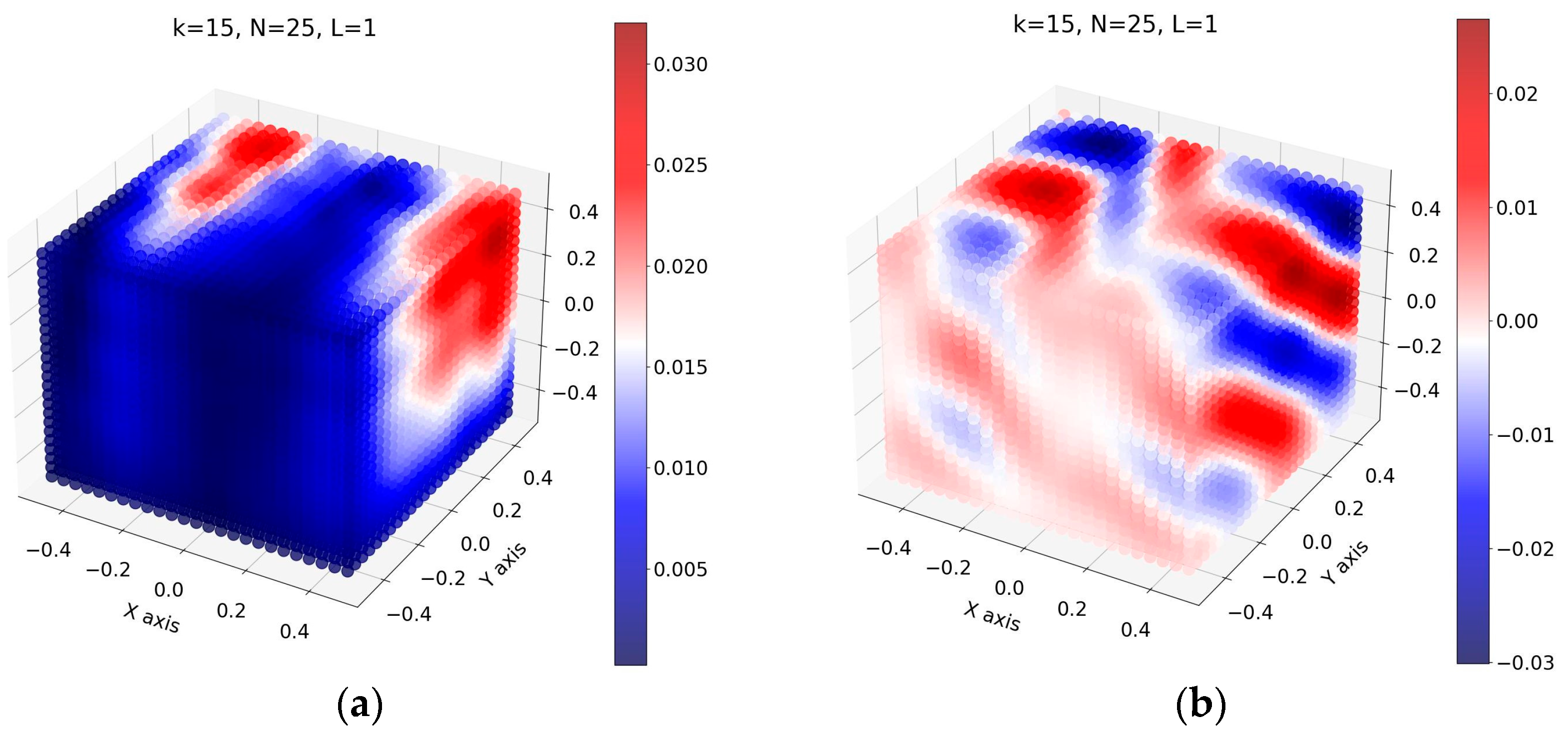
Figure 1. The total number of obtainable elementary partitions in such a case is
. The figure shows the obtained solution
as a result of convergence of iterations for Equations (24)–(27). The first sub-drawing in
Figure 1a shows the values of the
of the potential field modulus in the center of each cube, which vary in the range of
. The gradation of these values is also highlighted in the graph. The sub-drawing
Figure 1b shows the real part of the complex scalar field
whose values vary in the range
According to the character of the obtained picture, we obtain the expected type of the solution. In
Figure 1b, one can notice the refraction of the plane wave Equation (29) incident from the point of
against the boundary located at the point along the axis
In the limit
how the refracting wave changed the direction of its propagation can be seen, and as it passed within this region it experienced attenuation, due to which both the modulus of its value and the amplitude of its real values decreased. After passing through the point
the propagation resumes due to the run-up of the plane wave front, as in Equation (29).
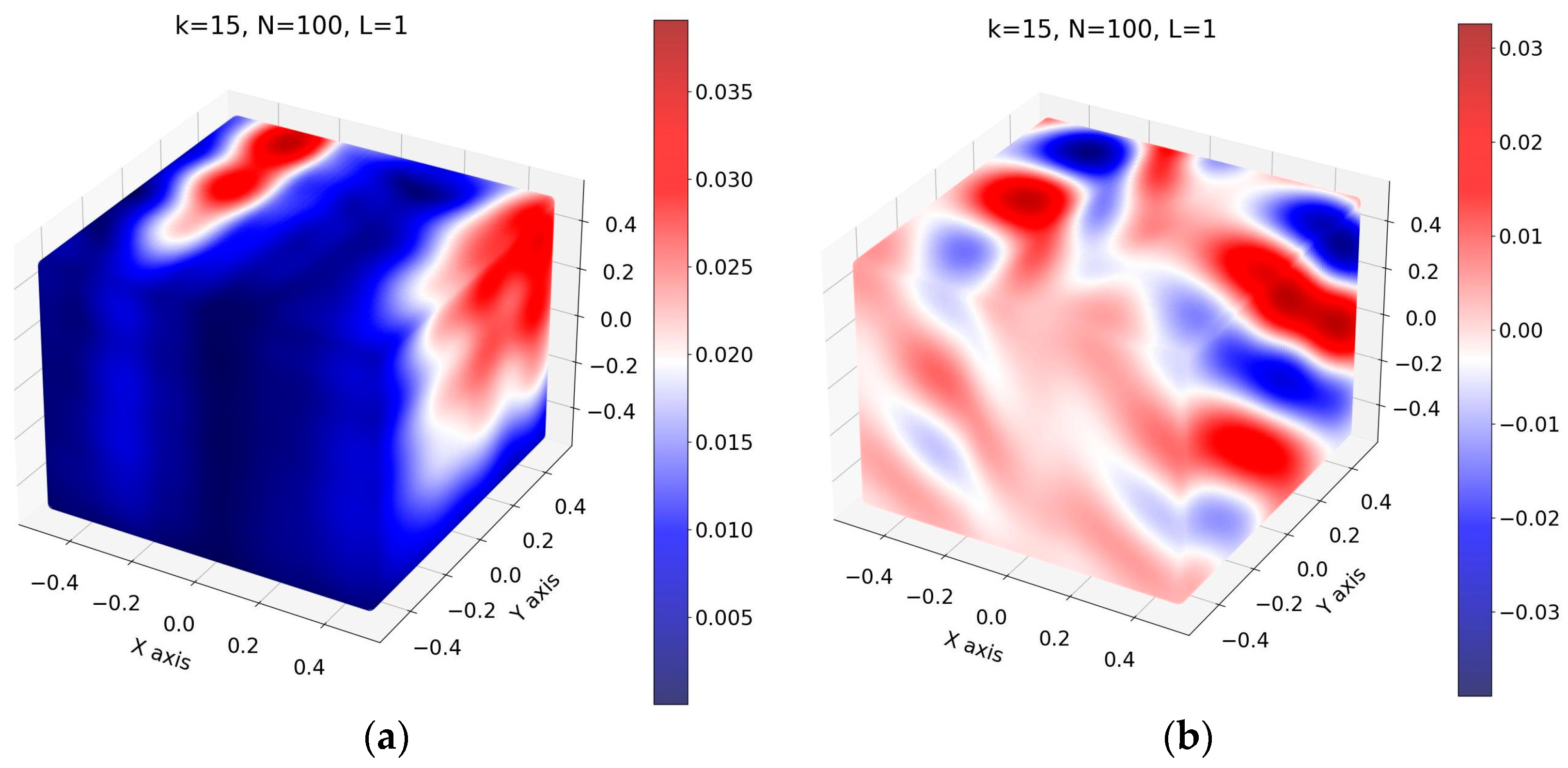
We also visualize the obtained results with a sufficiently large
in
Figure 2. The limits of the scalar field values remained the same, and also the obtained structure for the solution remained unchanged. The total number of obtainable elementary partitions in this case amounted to
.
As a result, having increased the linear partitioning of the domain by approximately a factor of 4, we obtain a 64-times increase in the discretization of the domain in view of which the obtained solutions show more features at the refraction boundary. Let us note the smoothness of the obtained solution, as a result of which it is possible to take into account small features both on the refraction boundary and on possible inclusions, whose sizes do not exceed the linear sizes of the obtained partitions .
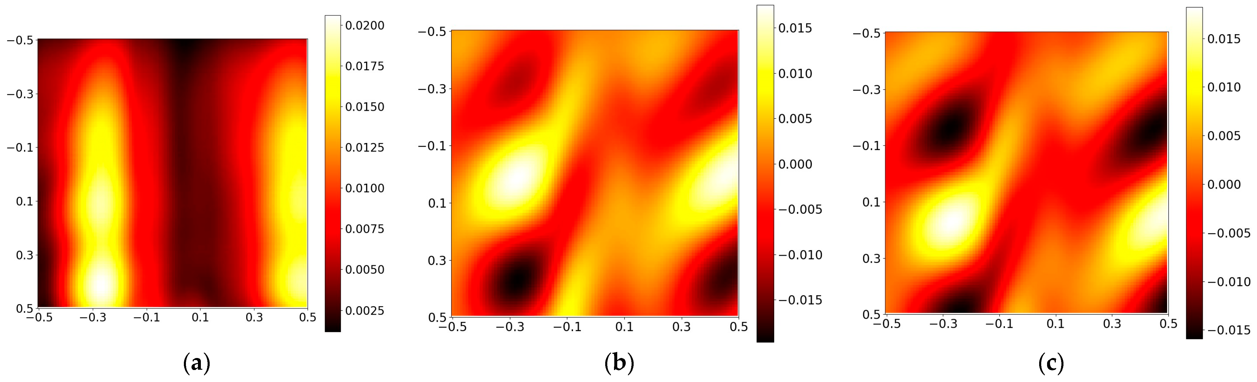
On the center slices on the axis
areas
in
Figure 3, we also see the picture of the refraction and attenuation of the wave, both in the modulus value,
Figure 3a, and in the values of amplitudes of the real
Figure 3b and the complex part of the wave
Figure 3c. On the graph of the modulus approximation of the scalar field values
Figure 3a, we can clearly see the transition in the range of
, which is a consequence of the transition of the refraction value in this region. In
Figure 3b,c, we see refraction in the pattern of propagation of the plane wave, as well as the attenuation of the amplitude of the scalar field values within
.
Performing calculations with different degrees of discretization of the solution domain, we measure the efficiency of the presented iterative method, Equations (24)–(27), using values of different metrics. For solutions with different discretization of the domain we measured the total number of matrix multiplications by the vector during the algorithm operation, the relative error of approximations of iterations counted by (28), the norm of incoherence of the obtained approximate solution , and the maximum value of the modulus of the scalar field . In addition to the above metrics, we measured the program execution time in seconds () for a given discretization () of the volume area of the solution on a personal computing device with an intel core i5-10400f processor and DDR4 RAM, with a frequency of 3200 MHz and a volume of 32 GB. Time was measured via the implementation of a C++ program in a sequential single-threaded execution of instructions.
Table 1 demonstrates the values of the above metrics for different numbers of partitions
source region
.
According to the results, we note that there is no dependence of the investigated values of the metrics on the number of partitions of the solution domain. It is shown that the number of matrix multiplications by vector necessary to obtain an approximation with a predetermined accuracy does not increase depending on the number of partitions of the domain . However, we observe an oscillation of this value, which may be due to a poor choice of cube sizes, which resulted in an inaccurate description of the refraction region.
Metrics , do not change depending on the number of partitions; we can only note the low value of the norm of non-convexity of the integral operator with respect to the obtained solution at small discretizations ᴎ . This circumstance can also be related to the number of final calculations or to a weak description of the solution domain of the problem. The index also varies within the error limits.
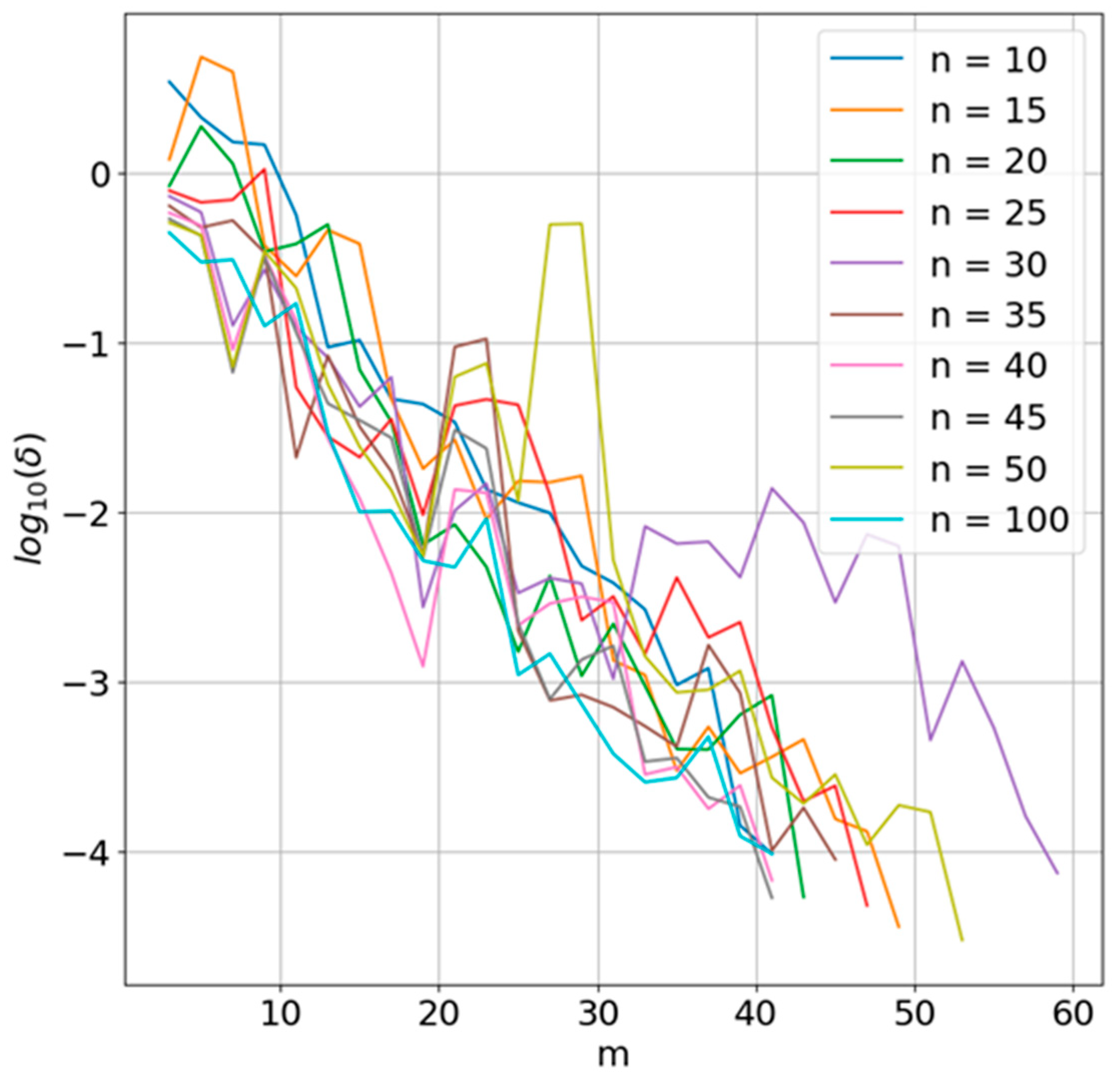
We display the graphs of the metric Equation (28) of the relative error
of approximations during the iterative method for Equations (24)–(27) depending on the number of applications of the matrix-to-vector multiplication operation
.
Figure 4 shows the value of
depending on
due to the exponential nature of the reduction of this metric. By prologarithmizing
we see the convergence pattern of the method in Equations (24)–(27) for the problem in Equations (29)–(30), in the values of powers of 10 of the base of the number system.
In the linearized dependence shown, we see by the convergence pattern in
Figure 4 an oscillating graph of metric Equation (28), demonstratively converging (in natural values) to the required value of approximation accuracy
. It can be seen from the graph that, with increasing discretization (n on the graph is equal to
or
,
or
) of the initial domain, the number of iterations (matrix-to-vector multiplications) does not increase, which cardinally contributes to the speed in solving the initial formulation of the integral equation at large discretizations.


