Oscillator Simulation with Deep Neural Networks

Abstract

The motivation behind this study is to overcome the complex mathematical formulation and time-consuming nature of traditional numerical methods used in solving differential equations. It seeks an alternative approach for more efficient and simplified solutions. A Deep Neural Network (DNN) is utilized to understand the intricate correlations between the oscillator’s variables and to precisely capture their dynamics by being trained on a dataset of known oscillator behaviors. In this work, we discuss the main challenge of predicting the behavior of oscillators without depending on complex strategies or time-consuming simulations. The present work proposes a favorable modified form of neural structure to improve the strategy for simulating linear and nonlinear harmonic oscillators from mechanical systems by formulating an ANN as a DNN via an appropriate oscillating activation function. The proposed methodology provides the solutions of linear and nonlinear differential equations (DEs) in differentiable form and is a more accurate approximation as compared to the traditional numerical method. The Van der Pol equation with parametric damping and the Mathieu equation are adopted as illustrations. Experimental analysis shows that our proposed scheme outperforms other numerical methods in terms of accuracy and computational cost. We provide a comparative analysis of the outcomes obtained through our proposed approach and those derived from the LSODA algorithm, utilizing numerical techniques, Adams–Bashforth, and the Backward Differentiation Formula (BDF). The results of this research provide insightful information for engineering applications, facilitating improvements in energy efficiency, and scientific innovation.

1. Introduction

There is a special place for dynamical systems [1], as well as for the identification of dynamical systems [2], in assessing physical phenomena in the realm of experimental science. Although many methods are used to model, simulate, and solve dynamical systems [3] and to discuss their stability [4], neural network-based techniques [5,6] to approximate the solution of DEs occurring in various systems [7] have, however, garnered a reputation in recent years. Other analytical methods for ordinary DEs [8] and partial DEs [9], semi-analytical methods [10], including the Variational Iteration Method (VIM) by using the Laplace Transform [11], and numerical methods have their own shortcomings in terms of convergence, precision, processing time, and computational complexity. However, a DNN [12] resolves these problems and, rather than through direct calculation, features are successfully acquired by the neural network through a training process in the layers of connected neurons [13]. In this study, we have evaluated the overall performance of a DNN for simulating the behavior of dependent variables occurring in the differential equation governed by a dynamical system. Few researchers have used trial solutions in their methodology which meet the initial or boundary conditions involved in the DEs [14]. This methodology of using a neural network in the solution of DEs is frequently attributed to them [15]. However, utilizing DNNs in different areas of daily life is challenging in terms of modeling and simulation. Our main focus is on analysis of the performance of the DNN-based methodology for harmonic oscillator simulation in a mechanical system. This technique has undergone numerous changes in the past to increase precision, but, to avoid the manual labor of computation, there must be computer software that enables less manual computation and efficient time management.

Some researchers have used a feed-forward neural network and a local optimization procedure in order to solve ordinary differential equations, systems of ordinary differential equations, and partial differential equations [16]. For the solution of DEs, neural networks, formed through grammatical evolution, were introduced by Tsoulos et al. [17]. This method employs grammatical evolution techniques [18] to evolve both the neural network structure and its parameters. Given the interest in developing neural networks for solving DEs, a user-friendly software program that allows researchers to quickly set up and solve questions would be very beneficial. We took advantage of the well-known programming language Python [19], which is widely used by professionals in various fields, especially in machine learning [20,21], and it plays an important role in solving DEs [22]. It gives users the freedom to use it for both straightforward and challenging issues. By implementing the outstanding Python program NeuroDiffEq [23], which was created specifically for the modelling of differential equations, we utilized a cutting-edge methodology [24]. The DNN-based strategy proposed in this study does not require explicitly feeding the problem information, and there is no need to explicitly give the initial or boundary condition for DEs. The trial solution satisfies initial and boundary conditions as well.

Applying a DNN-based method on DEs governed by a mechanical system is an interesting means to examine the behavior of an oscillator with respect to different parameters. We present two applications, the Van der Pol equation [25] and the Mathieu equation [26], which are derived from nonlinear and linear harmonic oscillators [27], respectively, to validate our approach of using a DNN to simulate a dynamical system. However, apart from the dynamical system, the Mathieu Equation is also linked to other subjects, such as applied and computational mathematics [28] and many engineering fields [29], due to the wide variety of its uses and the methods needed for qualitatively analyzing it. The Van der Pol equation, however, finds applications in many different industries like electronics, communication systems, and biological systems because of its capacity to record intricate dynamics [30].

A DNN solves a DE by considering it as an optimization problem [31]. The aim of a DNN when solving a DE is to reduce the residuals of the DE. These residuals are quantified by a loss function [32] that captures the discrepancy between the true and predicted values. Various loss functions [33] can be used to calculate the residuals, such as mean absolute error [34], L2 loss function [35], and A Unit Softmax loss [36].

To capture the periodic behavior effectively, the sine activation (SinActv) function [37] is an appropriate choice of activation function [38,39]. It is the typical trigonometric function ($f\left(x\right)=\sin \left(x\right)$), that applies a sine to its input values. It gives the best results for problems of an oscillatory nature, like harmonic oscillators. Closely similar modification in this way is also favorable for solving a number of dynamical structures, including vibration and dynamic control offered by [40], to analyze the impact of gyrotactic microorganisms [41] and evaluate the periodicity of nano/microelectromechanical systems oscillators [42].

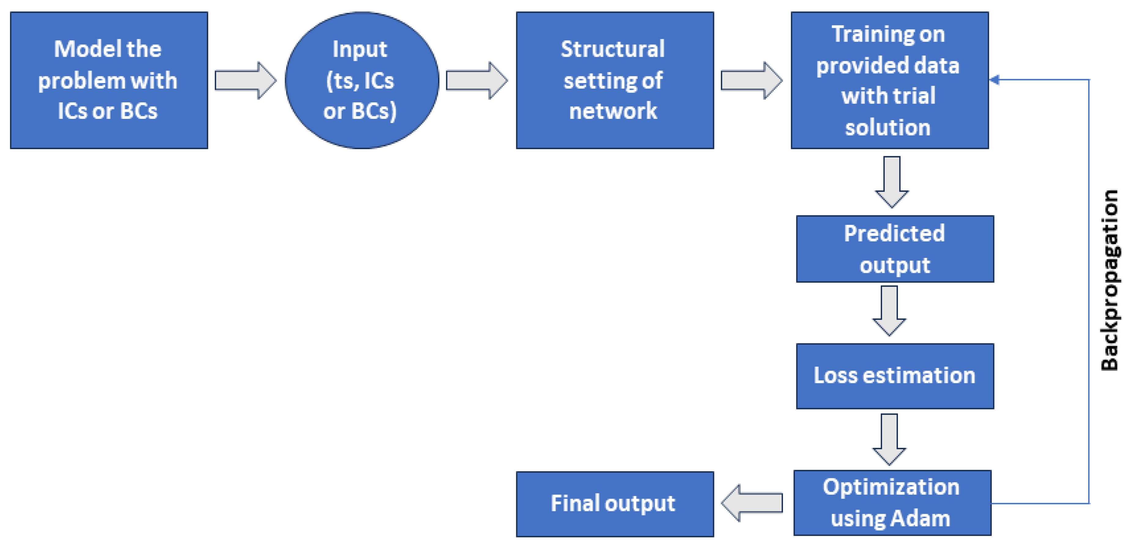
2. Structural Configuration and Method

NeuroDiffEq is a Python package constructed utilizing PyTorch, which employs ANNs to tackle both ordinary and partial differential equations (ODEs and PDEs). NeuroDiffEq streamlines problem-solving by emphasizing the problem domain for defining differential equations and initial/boundary conditions. It also provides flexibility for users to explore solution strategies, including ANN architecture and training parameters. NeuroDiffEq is not limited to a fixed architecture, but is designed to be versatile, allowing users to construct various types of neural network architectures. In our approach, a Fully Connected Neural Network (FCNN) [43], the most basic type of DNN [44], is leveraged as an approximating tool for dependent variables. An FCNN is structured in such a way that all neurons in a layer are fully connected to all neurons in the subsequent layer. This architecture allows information to flow through the network without skipping any neurons, making it a straightforward and densely interconnected structure. This network in the FCNN does not have any restrictions on connections between neurons in different layers, allowing for a comprehensive information flow throughout the network. Utilizing NeuroDiffEq to assess the mathematical models of dynamical systems outlined in Section 3.1 and Section 3.2, we carried out various experiments. The working rule for NeuroDiffEq is that once the network is fed with the input values, the NNs are trained to learn the underlying patterns in the data generated by the differential equations by using a trial solution which takes care of initial or boundary conditions as well. The differential equation is formulated as an optimization problem which is to be minimized. The trial solution is fed into the residual of the differential equation which is then minimized as much as possible to attain the approximated solution of the differential equation. We split our experiments into distinct instances based on the varying values of the parameters used in Equations (3) and (9). Our methodology elucidates the process of approximating solutions to DEs through the utilization of an FCNN in a more comprehensive manner, as illustrated in the flowchart in Figure 1 below.

In order to dive deeper into the proposed methodology, we shall discuss all the steps mentioned in the above flowchart in detail. By ‘structural setting of the network’, we mean the number of layers and the number of units in each layer, the number of epochs, activation function, loss function, optimizer, learning rate, etc. The methodology consists of following steps:

I. 

Preparation

Provide a comprehensive dataset (X, Y), which consists of input features X and corresponding dependent variable values Y, to train the FCNN with diverse input signals and operational conditions. Split the dataset into training and testing folders to validate the performance of the model. The situations included in this dataset span a wide variety of amplitudes, frequencies, and nonlinearities.

II. 

Launching the model

Initialize the model parameters of the FCNN, including weights, biases, learning rate, and number of epochs. Set the number of input units corresponding to the input features and output units in the layer according to the dependent variable. Our suggested neural network design has one input unit of network because there is only one independent variable in each DE presented in Section 3.1 and Section 3.2. The number of output units is also one, depending upon the dependent variable which is only one (for each DE). Three hidden layers are involved in our network, making it a deep neural network. Each hidden layer contains 16 units of neurons in total.

III. 

Forward propagation

For each epoch, perform forward propagation to obtain the output of the model, including applying the activation function to introduce nonlinearity. The choice of SinActv facilitated smooth transitions and continuous gradients during training because SinActv is continuous and smooth. The sine function’s smoothness enables effective optimization and aids in avoiding problems, such as disappearing or bursting gradients, which can impede training. Moreover, it accelerates the convergence rate.

IV. 

Estimating loss

Calculate the loss between the true and predicted values of the output of the training set. Update the cumulative loss using an appropriate loss function. To calculate residuals, we used the L2 loss function, which is the average of the squared difference between the true and predicted values.

V. 

Backpropagation

Compute the gradients of weights and biases with respect to loss by performing backpropagation, propagating the gradients backward and updating weights and biases accordingly.

VI. 

Optimization

Use an optimization algorithm to update the parameters. Utilizing the dataset, the FCNN is trained using cutting-edge training methods, including regularization and optimization algorithms, to improve its performance and generalization skills. This step helps to minimize the loss calculated during the training process. An Adam algorithm [45] with a learning rate of 0.001 is adapted to train on distinct points for each epoch that is produced by adding Gaussian noise [46] to the evenly distributed points on the t domain.

VII. 

Assessment of the model

After training a specified number of epochs, analyze the performance of the model using a testing set, which includes calculation of the average loss and evaluation of the accuracy of the model.

VIII. 

Prediction

Pass the input characteristics once the training procedure is complete to forecast the dependent variable’s output for unseen data.

The outlined strategy is translated into a structured algorithm proposed to estimate the dependent variables inherent in the intricate dynamics of the system under examination. This algorithm, Algorithm 1, serves as a precise computational framework, enabling accurate approximations crucial for in-depth analysis and modeling.

Algorithm 1: FCNN Training and Prediction.

I. Preparation # Load and Split dataset (X, Y) into training and testing sets X_train, X_test, Y_train, Y_test = train_test_split(X, Y, test_size = $n_1$, random_state = $n_2$) II. Launching the model # Initialize FCNN parameters input_units = X_train.shape [1], ${\mathbb{N}}_1$ output_units = ${\mathbb{N}}_2$ hidden_units = [${\mathbb{N}}_3$, ${\mathbb{N}}_4{,\mathbb{N}}_5$] learning_rate = $\mathbb{L}$ epochs = $\mathbb{E}$ visualization_frequency = M $\mathbb{W}$ = initialize_ $\mathbb{W}$ (${\mathbb{N}}_1$, [${\mathbb{N}}_3$, ${\mathbb{N}}_4{,\mathbb{N}}_5$], ${\mathbb{N}}_2$) $\mathbb{B}$ = initialize_ $\mathbb{B}$ ([${\mathbb{N}}_3$, ${\mathbb{N}}_4{,\mathbb{N}}_5$], ${\mathbb{N}}_2$) III. Forward Propagation for epoch in range(epochs): hidden_layers_output, model_output = forward_propagation(X_train, $\mathbb{W}$, $\mathbb{B}$) $\mathbb{y}$ = $\mathbb{A}$(model_output, $\mathbb{A}\_func$ IV. Estimating Loss $\mathbb{L}$ = calculate_ $\mathbb{L}$ (Y_train, $\mathbb{y}$, $\mathbb{L}\_func$ V. Backpropagation $\mathbb{G}$ = calculate_ $\mathbb{G}$ (X_train, hidden_layers_output, Y_train, $\mathbb{y}$) VI. Optimization $\mathbb{W}$, $\mathbb{B}$ = update_parameters ($\mathbb{W}$, $\mathbb{B}$, $\mathbb{G}$, $\mathbb{L}$) # Visualization if $\mathbb{E}$ % M == 0: print (f’Epoch: { $\mathbb{E}$ }, $\mathbb{L}$: { $\mathbb{L}$ }’) VII. Assessment of the Model hidden_layers_output, test_predictions = forward_propagation(X_test, $\mathbb{W}$, $\mathbb{B}$) test_ $\mathbb{L}$ = calculate_ $\mathbb{L}$ (Y_test, test_predictions, $\mathbb{L}\_func$) accuracy = evaluate_accuracy(Y_test, test_predictions) print (f’Average Test, $\mathbb{L}$: {test_, $\mathbb{L}$}’) print (f’Accuracy: {accuracy}%’) VIII. Prediction # Pass input characteristics for prediction unseen_data = load_unseen_data() $\mathbb{y}$ = predict_output(unseen_data, $\mathbb{W}$, $\mathbb{B}$) print ($\mathbb{y}$ for Unseen Data: { $\mathbb{y}$ }’) Activation function = $\mathbb{A}$, Predicted output = $\mathbb{y}$, Weights = $\mathbb{W}$, Gradients = $\mathbb{G},$ Biases = $\mathbb{B}$

Utilizing the above-mentioned algorithm, the DNN-based simulator shows amazing precision in predicting the behavior of both linear and nonlinear harmonic oscillators once it has been trained. NeuroDiffEq, a state-of-the-art Python package developed using PyTorch and designed to answer both ordinary and partial DEs of either a linear or nonlinear nature, is used to model the findings. It boosts efficiency and creates a comfortable environment for users so they can focus on the key aspect of concern. All these settings can be adjusted by the user, according to the nature of the given problem.

3. Application: Mathematical Models

It is observed that the neural network structure is favorable for handling a number of challenges in the area of computer vision and dynamical systems. Dynamical systems are constructed on the basis of modeling physical phenomena, and the mathematical models are considered to predict the behavior of a real structure. While a neural network-based structure is flexible to deal with standard linear and nonlinear problems, a complex nonlinear structure is considered a challenging problem for a neural network. We have found a way to deal with these challenges, a kind of blueprint for our neural networks. What is special about it is that it is designed to tackle these complex, nonlinear problems head-on. It is not just a theoretical idea; it is practical and can be put into action straight away. Our proposed architecture is favorable, directly implementable, and is not rigid; we can adjust and fine-tune various aspects of this blueprint based on what we need, whether it is the initial or boundary conditions of our problem or the limits we want to set. So, it is a bit like having a really smart, adaptable assistant that helps us solve these complex puzzles effectively.

In our study we considered linear and nonlinear DEs governed by harmonic oscillators from a mechanical system. To adopt the proposed structure, we used a modified form of the highly nonlinear mathematical model from a mechanical system, having the general form

$$x^{″}\left(t\right)+\zeta x^{\prime }\left(t\right)+{{\omega }_n}^{2}x=0$$

(1)

where $x\in {\mathbb{R}}^n$, $\zeta$ $(0<\zeta <\infty$) is a positive real number acting as a scaling factor to control the damping effect, ensuring the system’s behavior aligns with real-world mechanical constraints, ${\omega }_n$ is a positive real number (${0<\omega }_n<\infty )$ representing natural frequency, and ′ represents the derivative with respect to ‘t’.

To consider it a complex problem, the nonhomogeneous part should be in the shape of

$$x^{″}\left(t\right)+\zeta x^{\prime }\left(t\right)+{{\omega }_n}^{2}x=F\left(t\right)$$

(2)

$F\left(t\right)$ is the external forcing function; it may be a constant function, an exponential or sinusoidal function, or any other mathematical function. The captivating aspect of our study emerged when we explored the intriguing effects of $F\left(t\right)$ by infusing sinusoidal behavior into the mix.

Extending this strategy, in Section 3.1 and Section 3.2 we explore two distinct mathematical models regulated by differential equations (DEs) describing linear and nonlinear oscillatory behaviors in harmonic oscillators.

We considered two examples of oscillators for linear and nonlinear DEs and configured the neural network for each problem according to the abovementioned algorithm.

Table 1. Overview of the parametric settings in the neural network configurations for each respective problem.

Parameters	For Oscillator 1	For Oscillator 2
Input units (${\mathbb{N}}_1$)	1	1
Hidden units ([${\mathbb{N}}_3$, ${\mathbb{N}}_4{,\mathbb{N}}_5$])	(64, 64, 64)	(16, 16, 16)
Output units (${\mathbb{N}}_2$)	1	1
Learning rate ($\mathbb{L}$)	0.001	0.001
Activation function ($\mathbb{A}$)	SinActv	SinActv
Number of epochs ($\mathbb{E}$)	20,000	10,000
Loss function ($\mathbb{L}$)	L2	L2
Optimizer ($\mathbb{o}$)	Adam	Adam

provides a detailed summary of the specific settings used in the neural network for every problem we studied. These settings are like the unique instructions we give to the neural network to help it solve each particular problem accurately and efficiently. Table 1 offers a clear view of these essential details, allowing us to understand how the neural network is configured for different tasks.

3.1. Van der Pol Equation (Oscillator 1)

The Van der Pol equation is a second order nonlinear differential equation that traces the motion of a nonlinear harmonic oscillator and is represented mathematically in Equation (3).

$$x^{″}\left(t\right)+ϵ(c_0+c_1\cos (\omega t)+\alpha x^2\left)x^{\prime }\right(t)+{{\omega }_n}^{2}x=f_0+f_1\sin \left(\omega t\right)$$

(3)

The initial conditions are

$$u\left(0\right)=0, u^{\prime }\left(0\right)=2$$

(4)

If we relate Equation (3) with Equation (2), $F\left(t\right)=f_0+f_1\sin \left(\omega t\right)$ is the external force term and $\zeta =ϵ(c_0+c_1\cos (\omega t)+\alpha x^2)x^{\prime }$ introduces the damping effect. The terms involved in a parametrically damped Van der Pol Equation (3) are $x^{″}$, which represents acceleration of the system, while the whole term $(c_0+c_1\cos (\omega t)+\alpha x^2\left)x^{\prime }\right(t)$ is responsible for the damping force which depends on three factors, $c_0$, which describes resistance due to linear damping, $c_1\cos (\omega t)$, which is responsible for the sinusoidal variation of the damping coefficient, and $\alpha x^2$, which introduces nonlinear damping due to the square of the displacement of system. In this case, $ϵ$ is the scaling factor that regulates the damping effect’s intensity, while the term ${{\omega }_n}^{2}x$ is the spring force which involves the stiffness of the system. The displacement term, $\omega$, is the excitation frequency, and ${\omega }_n$ is the natural frequency. The right side of Equation (3) involves external forces, $f_0$ the constant force and $f_1\sin \left(\omega t\right)$ the sinusoidal force.

We conducted a comparative analysis between the oscillatory behavior generated by the solution of Equation (1) using a DNN-based approach and the results acquired by the implementation of the LSODA algorithm [47]. Our experimental setting comprises two major cases: parametric excitation in the absence of external excitation and parametric excitation in the presence of external excitation.

3.2. Mathieu Equation (Oscillator 2)

Consider a vertically forced pendulum governed by the Mathieu Equation, a linear second order differential equation in its classical version drawn from a harmonic oscillator,

$$u^{″}\left(t\right)+(a+\beta \cos t)u\left(t\right)=0$$

(5)

The corresponding initial conditions are

$$u\left(0\right)=1, u^{\prime }\left(0\right)=0$$

(6)

where the term $a$ is the stiffness parameter, the term $\beta$ is responsible for the parametric excitation, and u is the dependent variable for amplitude. If the parametric excitation term is present, the pendulum undergoes forced vibrations, which may be stable or unstable depending upon the relationship of the parameters $a$ and $\beta$. Figure 2 represents the physical interpretation of the vertically forced pendulum.

In Equations (5) and (6) if the parametric excitation term is set equal to zero, i.e., $\beta =0$, then this harmonic oscillator resembles the simple harmonic oscillator [48] with a stiffness coefficient $a.$

4. Results

4.1. Behavior of Oscillations for Parametric Excitation (Oscillator 1)

In this particular case, we did not encounter external excitation governed by the right side of Equation (3). With incrementally varying values of the coefficient of sinusoidal damping represented by ${ c}_1$, we conducted experiments to examine the effect of increasing ${ c}_1$ on the behavior of oscillations, as depicted in Figure 3a,b. The illustrations in Figure 3a,b show graphically that the oscillatory patterns produced by the governing equations have quasiperiodic properties.

In the absence of external excitation, the behavior of the oscillations is solely determined by the interplay between the damping forces and the restoring spring force. The system will exhibit natural oscillations around its equilibrium position. These oscillations occur due to the initial conditions and the inherent properties of the system, without any external force driving the motion. We set the values of all the parameters occurring in Equation (3) such that $f_0=0,{ f}_1=0, ϵ=0.2, \alpha =1, c_0=-1.$ The frequencies are ${\omega }_n=1$, $\omega =0.12$. For case 1, we used $c_1=1$. The terms on the right side of Equation (3) vanish, and the resulting equation takes the following form

$$x^{″}\left(t\right)+0.2(-1+\cos (0.12t)+x^2\left)x^{\prime }\right(t)+x=0$$

(7)

For case 2, we used $c_1=3,$ while all other parameters are the same as for case 1, and the resulting equation becomes

$$x^{″}\left(t\right)+0.2(-1+3\cos (0.12t)+x^2\left)x^{\prime }\right(t)+x=0$$

(8)

In case 1, the oscillations behave like sinusoids and are less jerky than in case 2. The coefficient of sinusoidal damping, $c_1$, plays a crucial role in shaping the quasiperiodic properties of the oscillations. Increasing $c_1$ leads to amplitude modulation in the oscillations. By increasing the value of $c_1$(case 2), oscillations are shown to be disrupted; the amplitude is reduced for a period of time. The presence of $c_1$ in the damping term $ϵ(c_0+c_1\cos (\omega t)+\alpha x^2\left)x^{\prime }\right(t$) contributes to nonlinear damping. Moreover, the oscillations exhibit abrupt peaks at the beginning and end of the graph.

The training and validation losses for both cases are displayed in Figure 3 to give insight into the model’s performance during the learning process. A comparison between the DNN-based scheme and a numerically approximated solution using LSODA is presented in Figure 4a,b. It is obvious from the figures that there is a high degree of agreement between the approximations made by the DNN and those obtained by LSODA, which guarantees the exactness and accuracy of the proposed methodology.

4.2. Behavior of Oscillations for External Excitation (Oscillator 1)

For the second illustration of nonlinear harmonic oscillator 1, we took into account the effect of external excitation along with parametric excitation. Again, we divided this case into two subcases on the basis of values of $f_1$. The setting of parameters in the presence of external excitation is done in such a way that $c_0=-1, c_1=1, ϵ=0.2, \alpha =1, f_0=0.4$ and ${\omega }_n=1, \omega =0.12$.

For case 3, using $f_1=1,$ Equation (3) takes the following form

$$x^{″}\left(t\right)+0.2(-1+\cos (0.12t)+x^2\left)x^{\prime }\right(t)+x=0.4+\sin \left(0.12t\right)$$

(9)

while $f_1=1.7$ is used for case 4 and the resulting equation becomes

$$x^{″}\left(t\right)+0.2(-1+\cos (0.12t)+x^2\left)x^{\prime }\right(t)+x=0.4+1.7\sin \left(0.12t\right)$$

(10)

For cases 3 and 4, Equations (9) and (10) are plotted in Figure 5a,b. As depicted in Figure 5a,b, nonlinear harmonic oscillator 1 is richer in distortions in the presence of external excitation. Additionally, for Equations (9) and (10) more nonlinearity is observed in the graph.

Figure 6a,b give a comparative demonstration of the proposed DNN-based methodology and the numerical solution using the LSODA algorithm. The outstanding performance of the DNN-based method is clear from the graphical representation. Another noticeable point of the quasiperiodic oscillations is damping, which is greater in the presence of external force as compared to the case when external excitation is not present. An increase in the value of $f_1$ from 1 to 1.7 causes an increase in damping.

4.3. Effects of Parameters on the Oscillations of Oscillator 2

In this section, we examine the results obtained from our proposed technique in depth and we also provide a graphical comparison between the DNN-based method and the numerical solution obtained from LSODA. For harmonic oscillator 2, three different cases in our experiment are described below in detail.

As a case 1, we used $a=3$ and $\beta =1.2,$ and observed the results as shown in Figure 7a. Case 2 was created using $a$ = 2 and $\beta$ = 1, and the outcomes are depicted graphically in Figure 7b. Lastly, for case 3 we further decreased the values of the parameters, using $a$ = 0.25 and $\beta$ = 0.05. The graph for the third case is shown in Figure 7c.

The rhythmic behavior of oscillations is examined in Figure 7a–c for a range of parameter values. The training and validation losses are shown in the figures above for each time up to 10,000 epochs. By changing the network’s weights during the training process, this loss can be reduced; optimization methods are useful in this context. A comparison between the DNN-based approach and the numerical method is shown in Figure 8a–c.

The dotted lines in Figure 8a–c representing the DNN-based solution are fitted very well on the solid lines which represent the numerical solution of the differential equation for the three cases of our problem. All of the panels in Figure 8 show that, for the range of time and parametric values taken into consideration for this research, the DNN-based solutions for our problem compare favorably with those obtained from the LSODA algorithm. This guarantees the accuracy of the suggested method.

5. Discussion

In this paper, we have been concerned with analyzing how a DNN simulates the behavior of a differential equation governed by a mechanical system in the realm of dynamical systems. DNNs demonstrate enhanced accuracy in simulating complex mathematical models, showcasing their potential in capturing intricate patterns and behaviors within these systems, while LSODA, being a traditional numerical method, might struggle with highly complex systems. DNNs can potentially provide more accurate results in such cases. DNNs learn patterns directly from data, enabling them to adapt to underlying structures in the dataset. This data-driven approach can be advantageous in scenarios where the underlying equations are unknown or difficult to formulate. DNNs optimize computational resources and time by exhibiting faster convergence rates and enable quicker model training and prediction. Through DNNs, we gained deep insights into the underlying dynamics of the mathematical models. This knowledge helps in understanding the complex relationships within these systems. The overall findings of our study presented in this paper are listed below.

• We successfully applied the proposed algorithm of using an FCNN as the fundamental architecture of the DNN for approximating the solution of differential equations governed by linear and nonlinear harmonic oscillators. The ability of DNNs to make accurate predictions, even in nonlinear and dynamic scenarios, highlights their robustness in handling complex, real-world problems.
• Trained DNN models can generalize well to unseen data patterns, making them useful for predicting responses in scenarios not encountered during training.
• The proposed algorithm gives the best results using an appropriate architectural setting for the network, including number of units in input, output, and hidden layers, SinActv as the activation function, and Adam as the optimizer.
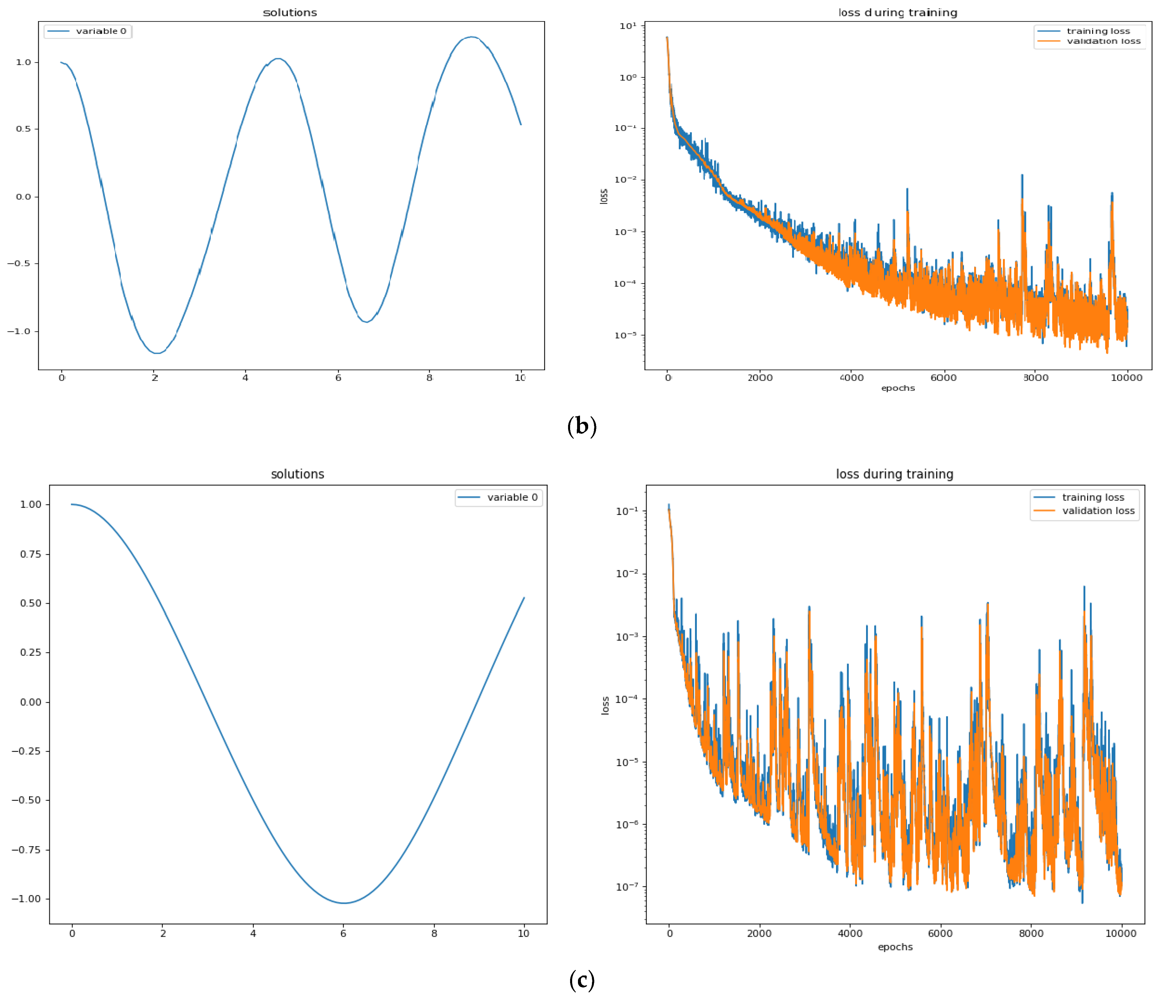
• During both the training and validation process, loss is evaluated. The observed loss values from graphical results are notably minimal, signifying the efficiency of the network’s performance during the training and validation procedures.
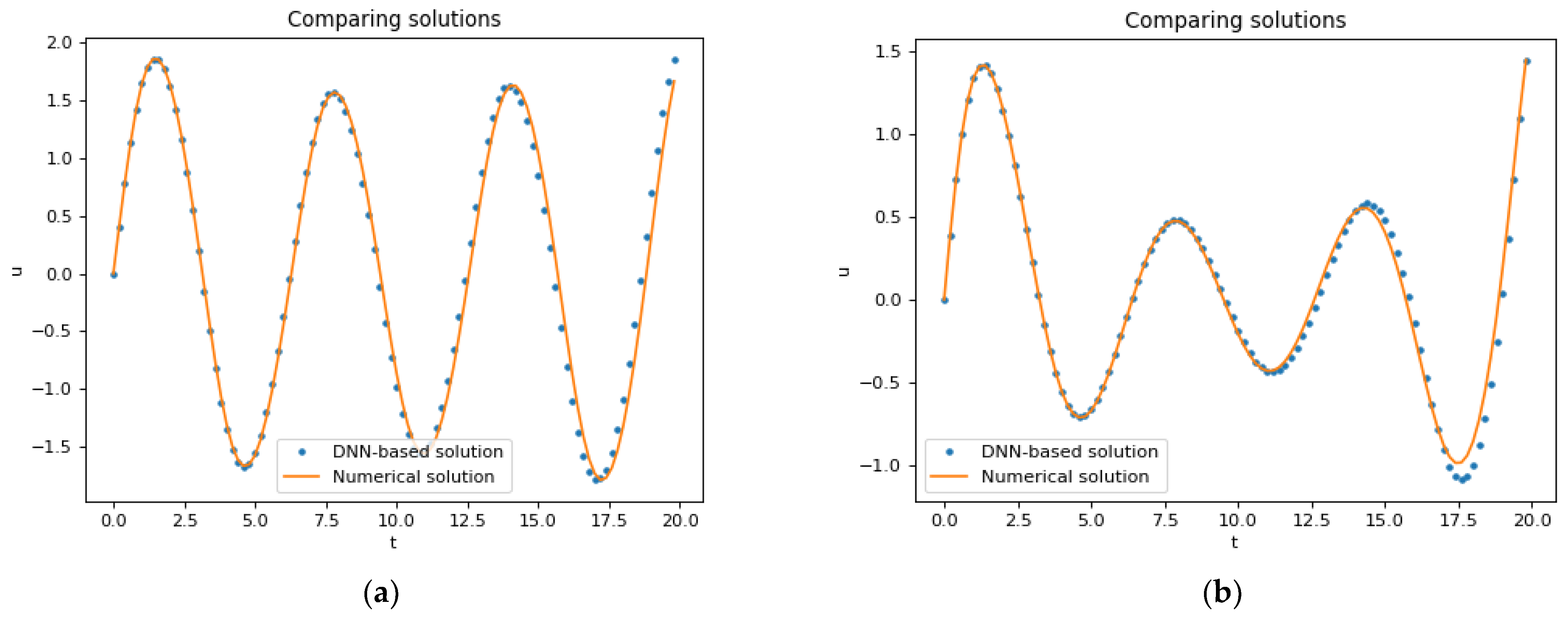
• To validate the proposed methodology, we performed a comparison of the DNN-based methodology with the LSODA algorithm, which is based on the numerical Adams–Bashforth method. It shows the discrepancy between the two methodologies.

Our study not only demonstrated the ability of DNNs in understanding complex mathematical models but also opened doors for their widespread application in research and practical domains. The insights gained from this study provide motivation for researchers to apply the proposed DNN-based scheme in different areas of dynamical systems, spanning diverse scientific domains such as physics, engineering, biology, climate science, and economics. The versatility of this approach offers the potential to revolutionize modeling and analysis techniques in these fields, fostering advancements and discoveries in each domain. However, DNNs, especially deep architectures, suffer from overfitting, where the model performs exceptionally well on the training data but poorly on new, unseen data. Techniques like regularization and validation are necessary to address this issue.

6. Conclusions

This study focuses on the simulation and analysis of linear and nonlinear dynamical systems using a flexible and reliable form of the DNN method. A refined neural structure is presented, based on a modified architecture of deep neural networks and an oscillating activation function to optimize the simulation of harmonic oscillators in mechanical systems. We specifically applied this approach to solving the Mathieu Equation and Van der Pol equation, representing linear and nonlinear harmonic oscillators. Comparing our DNN-based method to traditional numerical techniques, we concluded that the DNN-based approach, with carefully selected architecture and parameters, exhibited superior accuracy, ease of use, and faster convergence. The primary benefit of the suggested method is that, after the network has been trained, it enables instantaneous assessment of the solution at any desired number of points while consuming very little computational time. This cutting-edge method excels over other numerical methods in terms of accuracy and computational cost.

References

1. Qian, E.; Kramer, B.; Peherstorfer, B.; Willcox, K. Lift & learn: Physics-informed machine learning for large-scale nonlinear dynamical systems. Phys. D Nonlinear Phenom. 2020, 406, 132401. [Google Scholar]
2. Van den Bosch, P.P.J.; van der Klauw, A.C. Modeling, Identification and Simulation of Dynamical Systems; CRC Press: Boca Raton, FL, USA, 2020. [Google Scholar]
3. Abohamer, M.; Awrejcewicz, J.; Amer, T. Modeling of the vibration and stability of a dynamical system coupled with an energy harvesting device. Alex. Eng. J. 2023, 63, 377–397. [Google Scholar] [CrossRef]
4. Zhao, Y.; Jiang, C.; Vega, M.A.; Todd, M.D.; Hu, Z. Surrogate modeling of nonlinear dynamic systems: A comparative study. J. Comput. Inf. Sci. Eng. 2023, 23, 011001. [Google Scholar] [CrossRef]
5. Bukhari, A.H.; Sulaiman, M.; Raja, M.A.Z.; Islam, S.; Shoaib, M.; Kumam, P. Design of a hybrid NAR-RBFs neural network for nonlinear dusty plasma system. Alex. Eng. J. 2020, 59, 3325–3345. [Google Scholar] [CrossRef]
6. Ul Rahman, J.; Makhdoom, F.; Ali, A.; Danish, S. Mathematical modeling and simulation of biophysics systems using neural network. Int. J. Mod. Phys. B 2023, 2450066. [Google Scholar] [CrossRef]
7. Ul Rahman, J.; Danish, S.; Lu, D. Deep Neural Network-Based Simulation of Sel’kov Model in Glycolysis: A Comprehensive Analysis. Mathematics 2023, 11, 3216. [Google Scholar] [CrossRef]
8. Onder, I.; Secer, A.; Ozisik, M.; Bayram, M. On the optical soliton solutions of Kundu–Mukherjee–Naskar equation via two different analytical methods. Optik 2022, 257, 168761. [Google Scholar] [CrossRef]
9. Goswami, A.; Singh, J.; Kumar, D.; Gupta, S. An efficient analytical technique for fractional partial differential equations occurring in ion acoustic waves in plasma. J. Ocean. Eng. Sci. 2019, 4, 85–99. [Google Scholar] [CrossRef]
10. Iqbal, N.; Chughtai, M.T.; Ullah, R. Fractional Study of the Non-Linear Burgers’ Equations via a Semi-Analytical Technique. Fractal Fract. 2023, 7, 103. [Google Scholar] [CrossRef]
11. Rahman, J.U.; Mannan, A.; Ghoneim, M.E.; Yassen, M.F.; Haider, J.A. Insight into the study of some nonlinear evolution problems: Applications based on Variation Iteration Method with Laplace. Int. J. Mod. Phys. B 2023, 37, 2350030. [Google Scholar] [CrossRef]
12. Huang, Y.; Sun, S.; Duan, X.; Chen, Z. A study on deep neural networks framework. In Proceedings of the 2016 IEEE Advanced Information Management, Communicates, Electronic and Automation Control Conference (IMCEC), Xi’an, China, 3–5 October 2016. [Google Scholar]
13. Manogaran, M.; Louzazni, M. Analysis of artificial neural network: Architecture, types, and forecasting applications. J. Electr. Comput. Eng. 2022, 2022, 5416722. [Google Scholar]
14. Rackauckas, C.; Ma, Y.; Martensen, J.; Warner, C.; Zubov, K.; Supekar, R.; Skinner, D.; Ramadhan, A.; Edelman, A. Universal differential equations for scientific machine learning. arXiv 2020, arXiv:2001.04385. [Google Scholar]
15. Lagaris, I.E.; Aristidis, L.; Dimitrios, I. Fotiadis. Artificial neural networks for solving ordinary and partial differential equations. IEEE Trans. Neural Netw. 1998, 9, 987–1000. [Google Scholar] [CrossRef] [PubMed]
16. Tsoulos, I.G.; Gavrilis, D.; Glavas, E. Solving differential equations with constructed neural networks. Neurocomputing 2009, 72, 2385–2391. [Google Scholar] [CrossRef]
17. Tsoulos, I.G.; Gavrilis, D.; Glavas, E. Neural network construction and training using grammatical evolution. Neurocomputing 2008, 72, 269–277. [Google Scholar] [CrossRef]
18. O’Neill, M.; Ryan, C. Grammatical evolution. In IEEE Transactions on Evolutionary Computation; IEEE: Piscataway, NJ, USA, 2001; Volume 5, pp. 349–358. [Google Scholar]
19. Martelli, A.; Ravenscroft, A.M.; Holden, S.; McGuire, P. Python in a Nutshell; O’Reilly Media, Inc.: Sebastopol, CA, USA, 2023. [Google Scholar]
20. Hopkins, E. Machine learning tools, algorithms, and techniques. J. Self-Gov. Manag. Econ. 2022, 10, 43–55. [Google Scholar]
21. Herzen, J.; Lässig, F.; Piazzetta, S.G.; Neuer, T.; Tafti, L.; Raille, G.; Van Pottelbergh, T.; Pasieka, M.; Skrodzki, A.; Huguenin, N.; et al. Darts: User-friendly modern machine learning for time series. J. Mach. Learn. Res. 2022, 23, 5442–5447. [Google Scholar]
22. Nascimento, R.G.; Fricke, K.; Viana, F.A. A tutorial on solving ordinary differential equations using Python and hybrid physics-informed neural network. Eng. Appl. Artif. Intell. 2020, 96, 103996. [Google Scholar] [CrossRef]
23. Chen, F.; Sondak, D.; Protopapas, P.; Mattheakis, M.; Liu, S.; Agarwal, D.; Di Giovanni, M. Neurodiffeq: A python package for solving differential equations with neural networks. J. Open Source Softw. 2020, 5, 1931. [Google Scholar] [CrossRef]
24. Habiba, M.; Pearlmutter, B.A. Pearlmutter. Continuous Convolutional Neural Networks: Coupled Neural PDE and ODE. In 2021 International Conference on Electrical, Computer and Energy Technologies (ICECET); IEEE: Piscataway, NJ, USA, 2021. [Google Scholar]
25. Afzali, F.; Kharazmi, E.; Feeny, B.F. Resonances of a forced van der Pol equation with parametric damping. Nonlinear Dyn. 2023, 111, 5269–5285. [Google Scholar] [CrossRef]
26. Kovacic, I.; Rand, R.; Sah, S.M. Mathieu’s equation and its generalizations: Overview of stability charts and their features. Appl. Mech. Rev. 2018, 70, 020802. [Google Scholar] [CrossRef]
27. Rehman, S.; Hussain, A.; Rahman, J.U.; Anjum, N.; Munir, T. Modified Laplace based variational iteration method for the mechanical vibrations and its applications. Acta Mech. Autom. 2022, 16, 98–102. [Google Scholar] [CrossRef]
28. Yang, X.-S. Introduction to Computational Mathematics; World Scientific Publishing Company: Singapore, 2014. [Google Scholar]
29. El-Dib, Y.O.; Elgazery, N.S. Damped Mathieu equation with a modulation property of the homotopy perturbation method. Sound Vib. 2022, 56, 21–36. [Google Scholar] [CrossRef]
30. Luo, Z.; Bo, Y.; Sadaf, S.M.; Liu, X. Van der Pol oscillator based on NbO2 volatile memristor: A simulation analysis. J. Appl. Phys. 2022, 131, 054501. [Google Scholar] [CrossRef]
31. Gambella, C.; Ghaddar, B.; Naoum-Sawaya, J. Optimization problems for machine learning: A survey. Eur. J. Oper. 2021, 290, 807–828. [Google Scholar] [CrossRef]
32. Janocha, K.; Czarnecki, W.M. On loss functions for deep neural networks in classification. arXiv 2017, arXiv:1702.05659. [Google Scholar] [CrossRef]
33. Wang, Q.; Ma, Y.; Zhao, K.; Tian, Y. A comprehensive survey of loss functions in machine learning. Ann. Data Sci. 2020, 9, 187–212. [Google Scholar] [CrossRef]
34. Qi, J.; Du, J.; Siniscalchi, S.M.; Ma, X.; Lee, C.-H. On mean absolute error for deep neural network based vector-to-vector regression. IEEE Signal Process. Lett. 2020, 27, 1485–1489. [Google Scholar] [CrossRef]
35. Liu, L.; Li, P.; Chu, M.; Zhai, Z. L2-Loss nonparallel bounded support vector machine for robust classification and its DCD-type solver. Appl. Soft Comput. 2022, 126, 109125. [Google Scholar] [CrossRef]
36. Ul Rahman, J.; Ali, A.; Ur Rehman, M.; Kazmi, R. A unit softmax with Laplacian smoothing stochastic gradient descent for deep convolutional neural networks. In Intelligent Technologies and Applications: Second International Conference, INTAP 2019, Bahawalpur, Pakistan, 6–8 November 2019, Revised Selected Papers 2; Springer: Singapore, 2020. [Google Scholar]
37. Liu, X.; Zhou, J.; Qian, H. Short-term wind power forecasting by stacked recurrent neural networks with parametric sine activation function. Electr. Power Syst. Res. 2021, 192, 107011. [Google Scholar] [CrossRef]
38. Ul Rahman, J.; Makhdoom, F.; Lu, D. Amplifying Sine Unit: An Oscillatory Activation Function for Deep Neural Networks to Recover Nonlinear Oscillations Efficiently. arXiv 2023, arXiv:2304.09759. [Google Scholar]
39. Dubey, S.R.; Singh, S.K.; Chaudhuri, B.B. Activation functions in deep learning: A comprehensive survey and benchmark. Neurocomputing 2022, 503, 92–108. [Google Scholar] [CrossRef]
40. Do, N.-T.; Pham, Q.-H. Vibration and dynamic control of piezoelectric functionally graded porous plates in the thermal environment using FEM and Shi’s TSDT. Case Stud. Therm. Eng. 2023, 47, 103105. [Google Scholar] [CrossRef]
41. Rashid, U.; Ullah, N.; Khalifa, H.A.E.-W.; Lu, D. Bioconvection modified nanoliquid flow in crown cavity contained with the impact of gyrotactic microorganism. Case Stud. Therm. Eng. 2023, 47, 103052. [Google Scholar] [CrossRef]
42. Naveed, A.; Rahman, J.U.; He, J.-H.; Alam, M.N.; Suleman, M. An efficient analytical approach for the periodicity of nano/microelectromechanical systems’ oscillators. Math. Probl. Eng. 2022, 2022, 9712199. [Google Scholar]
43. Zhang, Y.; Lee, J.; Wainwright, M.; Jordan, M.I. On the learnability of fully-connected neural networks. In Proceedings of the 20th International Conference on Artificial Intelligence and Statistics, PMLR, Fort Lauderdale, FL, USA, 20–22 April 2017. [Google Scholar]
44. Yu, X.; Wang, Y.; Liang, J. A self-adaptive gradient descent search algorithm for fully-connected neural networks. Neurocomputing 2022, 478, 70–80. [Google Scholar]
45. Diederik, P.K.; Ba, J. Adam: A method for stochastic optimization. arXiv 2014, arXiv:1412.6980. [Google Scholar]
46. Majed, E.H.; Süsstrunk, S. Blind universal Bayesian image denoising with Gaussian noise level learning. IEEE Trans. Image Process. 2020, 29, 4885–4897. [Google Scholar]
47. Hindmarsh, A.C.; Petzold, L.R. Livermore Solver for Ordinary Differential Equations (LSODA) for Stiff or Non–Stiff System; Nuclear Energy Agency (NEA) of the Organisation for Economic Co-operation and Development (OECD): Paris, France, 2005. [Google Scholar]
48. Rushka, M.; Freericks, J.K. A completely algebraic solution of the simple harmonic oscillator. Am. J. Phys. 2020, 88, 976–985. [Google Scholar] [CrossRef]
Figure 1. Flowchart depicting the approach employed for harmonic oscillator simulation using an FCNN.
Mathematics 12 00959 g001
Figure 2. Physical interpretation of the vertically forced pendulum.
Mathematics 12 00959 g002
Figure 3. (a) DNN-based approximation of the solution of Equation (1) for case 1, when f 0 = 0 ,   f 1 = 0 ,   ϵ = 0.2 ,   α = 1 ,   ω n = 1 ,   ω = 0.12 ,   c 0 = 1 ,   c 1 = 1 , and loss during learning process. (b) DNN-based approximation of the solution of Equation (1) for case 2, when f 0 = 0 ,   f 1 = 0 ,   ϵ = 0.2 ,   α = 1 ,   ω n = 1 ,   ω = 0.12 ,   c 0 = 1 ,   c 1 = 3 , and loss during learning process.
Mathematics 12 00959 g003
Figure 4. (a) Comparison between the DNN-based method and the LSODA algorithm for nonlinear harmonic oscillator 1 for case 1. (b) Comparison between the DNN-based method and the LSODA algorithm for nonlinear harmonic oscillator 1 for case 2.
Mathematics 12 00959 g004
Figure 5. (a) DNN-based approximation of the solution of Equation (3) for case 3, when c 0 = 1 ,   c 1 = 1 ,   ϵ = 0.2 ,   α = 1 ,   ω n = 1 ,   ω = 0.12 ,   f 0 = 0.4 ,   f 1 = 1 , and loss during learning process. (b) DNN-based approximation of the solution of Equation (3) for case 4, when c 0 = 1 ,   c 1 = 1 ,     ϵ = 0.2 ,   α = 1 ,   ω n = 1 ,   ω = 0.12 ,   f 0 = 0.4 ,   f 1 = 1.7 , and loss during learning process.
Mathematics 12 00959 g005
Figure 6. (a) Comparison between the DNN-based method and the LSODA algorithm for nonlinear harmonic oscillator 1 for case 3. (b) Comparison between the DNN-based method and the LSODA algorithm for nonlinear harmonic oscillator 1 for case 4.
Mathematics 12 00959 g006
Figure 7. (a) DNN-based approximation of the solution of Equation (5) and the loss in the training and validation process for case 1 (a = 3, β = 1.2 ). (b) DNN-based approximation of the solution of Equation (5) and the loss in the training and validation process for case 2 (a = 2, β = 1 ). (c) DNN-based approximation of the solution of Equation (5) and the loss in the training and validation process for case 3 (a = 0.25, β = 0.05 ).
Mathematics 12 00959 g007aMathematics 12 00959 g007b
Figure 8. (a) Comparison between the DNN-based method and the LSODA algorithm for harmonic oscillator 2 for case 1 (a = 3, β = 1.2 ). (b) Comparison between the DNN-based method and the LSODA algorithm for harmonic oscillator 2 for case 2 (a = 2, β = 1 ). (c) Comparison between the DNN-based method and the LSODA algorithm for harmonic oscillator 2 for case 3 (a = 0.25, β = 0.05 ).
Mathematics 12 00959 g008