Abstract
Lightweight and adaptive adjustment are key research directions for deep neural networks (DNNs). In coal industry mining, frequent changes in raw coal sources and production batches can cause uneven distribution of appearance features, leading to concept drift problems. The network architecture and parameters should be adjusted frequently to avoid a decline in model accuracy. This poses a significant challenge for those without specialist expertise. Although the Neural Architecture Search (NAS) has a strong ability to automatically generate networks, enabling the automatic design of highly accurate networks, it often comes with complex internal topological connections. These redundant architectures do not always effectively improve network performance, especially in resource-constrained environments, where their computational efficiency is significantly reduced. In this paper, we propose a method called Topology Complexity Neural Architecture Search (TCNAS). TCNAS proposes a new method for evaluating the topological complexity of neural networks and uses both topological complexity and accuracy to guide the search, effectively obtaining lightweight and efficient networks. TCNAS employs an adaptive shrinking search space optimization method, which gradually eliminates poorly performing cells to reduce the search space, thereby improving search efficiency and solving the problem of space explosion. In the classification experiments of coal and gangue, the optimal network designed by TCNAS has an accuracy of 83.3%. And its structure is much simpler, which is about 1/53 of the parameters of the network dedicated to coal and gangue recognition. Experiments have shown that TCNAS is able to generate networks that are both efficient and simple for resource-constrained industrial applications.
Keywords:
Neural Architecture Search; lightweight neural network; topological complexity; multiobjective optimization; adaptive adjustment MSC:
68Q25; 68Q10
1. Introduction
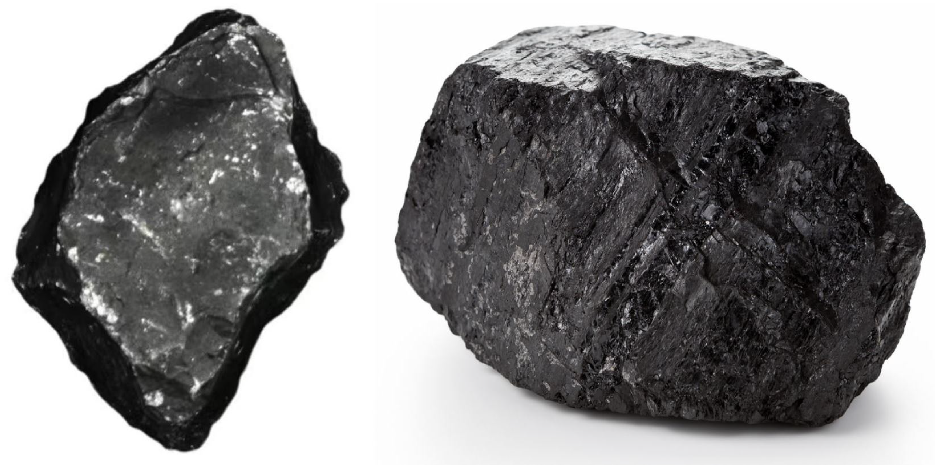
With the rapid development of the coal industry, the automated classification of coal and gangue becomes the key to enhancing production efficiency and protecting the environment. Gangue is solid waste produced during the process of coal mining. It is usually gray or black in color, contains low levels of coal, and is harder than coal. Due to the distinctive lustre and laminar structure of coal, coal and gangue have obvious textural differences in appearance, which can be effectively recognized by direct observation or by applying image recognition techniques. The appearance of coal and gangue is characterized in Figure 1. Traditional classification methods based on image processing and pattern recognition are increasingly applied in industrial production to address the harsh working conditions and inefficiency associated with the labor-intensive manual sorting of coal and gangue. Traditional machine learning methods [1], such as SVM, KNN, CART, and AdaBoost, are used to train the classifier based on processed feature data. However, the manual feature extraction required in traditional machine learning methods is time-consuming and prone to errors [2,3,4]. For this problem, several researchers [5,6,7,8,9] have deployed deep learning for the issue of coal and gangue recognition. Typically, deep-learning-based methods are able to achieve high accuracy in classifying coal and gangue because they use multi-layer convolution to enable automatic extraction of feature information.
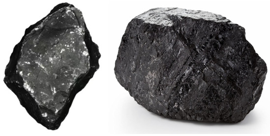
Figure 1.
Comparison of the appearance and characteristics of coal and gangue.
Deep learning techniques currently face a significant challenge in accurately distinguishing between coal and gangue. This difficulty arises primarily from the wide variety and variability in their appearance, which is influenced by their different sources. Coal, for instance, can come from various mines or geographical regions, leading to differences in glossiness, colors, and texture due to the geological types and mineral compositions unique to each source. These variations can cause a phenomenon known as concept drift, where the data distribution that the model was trained on does not align with the data encountered in real-world applications. This misalignment can lead to a decline in the model’s performance, as it struggles to adapt to the new appearances of coal and gangue. In the context of automatic identification systems for coal and gangue, this issue is compounded by the fact that models can only be trained on datasets representing a limited selection of coal sources and batches. When the appearance of coal deviates beyond the model’s trained range, it can significantly impact production efficiency and challenge the system’s recognition accuracy and stability.
Although noise reduction techniques, such as Laplace operators and Gaussian filtering [10], can be applied to enhance the robustness of the system and suppress the accuracy degradation to a certain extent, these methods often fail to ensure the continued stability of the system when the concept drift is significantly out of range. Therefore, the occurrence of concept drift means that the architecture and parameters of the neural network need to be adapted in a timely manner to accommodate data changes, a task that is both complex and time-consuming. This issue is particularly challenging for production personnel who lack specialized knowledge. Therefore, in the process of classifying coal and gangue, facing the phenomenon of concept drift, finding an effective strategy to adjust the architecture and parameters of the neural network has become a critical challenge.
NAS is powerful in searching high accuracy networks and has been applied in several fields such as computer vision [9,11,12,13,14,15,16,17,18], speech processing [19,20]. and natural language processing (NLP) [21,22]. However, the networks generated by NAS often comprise millions of parameters, which can consume significant memory resources and limit running efficiency when using limited computing resources. To address this problem, hardware-aware NAS [23] has been developed, focusing more on reducing computational costs such as latency, number of parameters, floating point operations per second (Flops), and memory footprint while maintaining a certain level of accuracy. However, ignorance of network architectural complexity makes hardware-aware NAS inadequate in reducing computational costs. The higher the complexity of the network architecture, the more nodes and edges its topology has, and therefore the more parameters it requires. As the computational cost of neural networks mainly comes from the updating and computation of parameters, the topology can directly affect the computational complexity of forward and backpropagation algorithms. Deeper or wider networks mean that more parameters need to be updated during training, which directly increases the computational cost. Networks with high topological complexity will contain a large number of layers and parameters, which not only increases the difficulty of training but also requires more computational resources when deployed. For example, although a network with multiple convolutional layers and intricate connection structures may exhibit outstanding performance in terms of accuracy, it could face limitations in applications within constrained hardware environments.
For the above difficult problems, there are shortcomings regarding NAS in the current related literature. First, the topological complexity is ignored while searching for and generating a lightweight network. This can lead to suboptimal results, as too simplistic networks may not be able to handle the complexity of real-world tasks. Second, the search space refinement can only be manually executed by experts. This is a time-consuming and resource-intensive process, making it difficult to guarantee the efficiency of search operations. Table 1 summarizes the advantages and limitations of various existing techniques. According to the table, despite the excellent performance of traditional methods and existing NAS technologies in some aspects, they still fall short when dealing with the complex and variable problem of coal and gangue classification. To overcome these issues, this paper proposes Topology Complexity Neural Architecture Search (TCNAS). TCNAS provides a more balanced and efficient solution by introducing topological complexity considerations. TCNAS does not rely on fine-tuning of the search space by human experts. It employs an adaptive search space shrinking mechanism that automatically refines the search space without involving experts. This helps to unleash the full potential of NAS, generating networks that are both lightweight and powerful, to tackle more challenging problems.

Table 1.
Comparison of different methods in coal and gangue classification tasks.
An improved NAS for considering both topological complexity and search efficiency is motivated by the above discussion. The main contributions of this work are as follows:
- This study proposes a novel complexity evaluation method for neural network topology. Since the number of neurons and the connections among them contribute to the overall complexity of the network architecture, an evaluation metric is calculated by mapping their features and internal structures.
- Regarding limited computational resources, this study proposes a Topology Complexity Neural Architecture Search (TCNAS) method to search and generate a lightweight network. This method can significantly reduce architectural parameters of networks and facilitate the generation of networks in a quick and simple way.
- An adaptive search space shrinking optimization method is proposed to enhance the search capability and efficiency. The method calculates the effectiveness of each cell of the overall search space, removes cells with poor effects, and retains high-quality cells to form an optimized search space. In this regard, the search efficiency is largely improved.
The remainder of this paper is organized as follows: Section 2 reviews relevant works and introduces the basic principles and applications of NAS technology. Section 3 describes the design and implementation of the TCNAS, including the evaluation method for the topology complexity of neural networks and the adaptive search space shrinking optimization method. Section 4 validates the effectiveness of the TCNAS method through experiments and compares it with existing technologies. Section 5 discusses the significance of TCNAS, and Section 6 concludes the research findings, summarizing the shortcomings and future research directions.
2. Related Work
2.1. Neural Architecture Search
Neural Architecture Search (NAS) stands at the heart of Automated Machine Learning (AutoML), focusing on the automated discovery of optimal deep neural network (DNN) architectures. The ultimate goal of AutoML is to minimize human intervention and optimize model selection and parameter tuning through an automated process, leading to more efficient machine learning model development. In this context, not only the field of NAS but also innovative approaches in other research areas [24] have shown the potential to reduce human intervention. Currently, NAS has demonstrated its powerful performance in tasks such as image classification [9,11,12,13,14,25,26,27,28,29], object detection [16,18], and semantic segmentation [15,17].
NAS consists of three components: search space, search strategies, and performance evaluation. The search space outlines all potential architectures, while search strategies guide the identification of the most effective architecture. Common search strategies include evolutionary algorithms (EA) [13,30], reinforcement learning (RL) [11], gradient-based methods [27], and Bayesian optimization [9,31]. Performance evaluation mechanisms are used to evaluate the performance of the searched architectures. AmoebaNet [13] compared RL-based NAS with EA-based NAS and showed that EA-based NAS can converge faster with the same hardware, especially in the initial phase of the search. Methods based on RL and EA consume huge computational resources, although they can achieve high architectural performance. AmoebaNet achieved better results on both the Cifar-10 dataset and the ImageNet dataset, but the search took 3150 GPU days. Compared with RL, gradient-based algorithms reduce the consumption of computational resources. ENAS [32] adopts a gradient-based search strategy to improve the search efficiency by parameter sharing, which reduces the search time to within one GPU day, but it requires the construction of a supernet in advance, which requires high expertise.
2.2. Search Space Design
In previous studies on NAS, much of the focus has been on refining search strategies. Yet, the construction of the search space plays a crucial and immediate role in shaping NAS effectiveness and the caliber of architectures it can uncover. The search space consists of a collection of networks defined by parameters such as network depth, types of operations, types of connections, kernel sizes, and the number of filters, where various operations are combined within the set to generate network architectures. It encompasses the entire set of possible operations for neural networks. A well-designed search space can elevate the upper limit of NAS performance and simultaneously increase the likelihood of discovering high-performance architectures.
However, there is a delicate balance between the size of the search space and its design. A smaller search space, if comprised of carefully selected decisions, can facilitate NAS in finding high-performance architectures more easily. However, this approach requires significant labor costs for human experts to design excellent search spaces and can also limit the ability of algorithms to discover truly innovative architectures. Conversely, a larger search space increases the probability of finding novel architectures but also requires longer search times and more computational resources.
In the early stages, Zoph et al. [11] adopted a NAS method based on RL, utilizing parameters such as the type, size, and connections of each layer in the network to construct a global search space. An RNN controller was employed to search and identify architectures with outstanding accuracy. However, its simultaneous search of a large number of parameters and architectures requires a large amount of computational resources, and its shortcomings in search efficiency and computational cost have motivated researchers to explore more efficient algorithms.
To reduce computational burdens, an effective approach is to transition from traditional global search methods into cell-based local search. NASNet [12] introduced this cell-based search framework, where the design of the search space involves stacking optimized cells, including normal and reduction cells, repetitively. This approach not only reduces the cost and enhances the efficiency of the search process but also enriches the diversity of the search space. NASNet constructs scalable architectures modularly through reusable normal and reduction cells. Normal cells maintain the size of the feature maps, whereas reduc cells downsample the input feature maps, halving their dimensions and reducing their spatial resolution. NASNet searches the above two optimal cells from the small dataset, cifar10, and extends the network architecture by increasing the number of cells and repeated stacking and successfully migrates them to the large dataset Imagine, with excellent performance, which improves the portability of NAS. After that, many studies [33] have adopted the cell-based search space design and improved it in several aspects.
Progressive Neural Architecture Search (PNAS) [34] inherits the methodology of NASNet, employing a progressive search strategy that starts from the smallest structures and iterates through them, incrementally increasing the scale of cell parameters for efficient exploration of the search space. Unlike the earlier NASNeT, PNAS reduces the search space by controlling the step size, and each stage concentrates on evaluating the architectures focused on those most likely to improve performance. Liu et al. proposed differentiable architecture search (darts) [27] based on NASNeT. Darts takes a continuous representation of the previously discrete search space and constructs a graph in the form of a supernet, where the operation with the highest probability of operation in the network is selected by gradient descent. This continuous search space allows darts to smoothly adjust the architecture throughout the search process.
However, many of the existing neural network architectures operate under a human-set framework, requiring human experts to predefine a cell with a sufficiently small range and high performance potential as the basis of the search space. This not only increases the human cost but also puts high demands on professional knowledge and has certain limitations. To address these issues, some studies on search space optimization methods have appeared in recent years. In the binary NAS algorithm proposed by EBNAS [35], it was found that convolutional operations are detrimental to search if they are too dominant, so it uses some search space simplifying strategies to ensure that the search is efficient. The activation distribution is adjusted by removing the BatchNorm and PReLU layers from the initial search space to improve the binary network performance. CNAS [28] leverages curriculum learning to gradually expand the search space, utilizing previously acquired knowledge to inform the exploration of larger spaces. Conversely, AutoSpace [29] employs a differentiable fitness function to assess cell performance and a differentiable evolutionary algorithm to refine the search space for future explorations. However, AutoSpace may face some challenges in optimizing the search space using EA, such as high redundancy and slow convergence rates. These issues primarily stem from the typically large scale of the initial search spaces, as EA tends to perform poorly when dealing with large search spaces. Actually, even using random searches may yield powerful results if there is a rich, but not overly broad, search space [27,36]. This process often involves repeated attempts and adjustments, so there is still a need for human involvement in search space optimization, and there is still a certain amount of manual intervention.
2.3. Computing-Cost-Aware NAS
In many domains, models obtained by NAS exhibit unprecedented accuracy. However, these high-performance models often contain millions of parameters and require billions of floating-point operations (Flops), making their deployment in scenarios with limited computational resources a significant challenge. In industrial applications requiring real-time performance, such as dynamic classification equipment for coal and gangue, these devices must detect objects in real time on conveyor belts and cannot afford the latency involved in sending data to the cloud and waiting for results.
Traditional approaches to NAS have tended to focus on network performance while ignoring the computing costs. This leads to a large number of redundant structures. However, in practice, computation costs and storage resources are often limited. The existence of redundant structures not only increases the computation and storage costs but may also negatively affect the performance improvement. For this reason, adopting a computation-cost-aware NAS method has significant practical value.
Computational-cost-aware NAS methods involve balancing computation cost and performance while searching for architectures. This method aims to identify architectures that maintain high performance at lower computational costs. By employing computational-cost-aware NAS methods, the computational and storage costs of neural networks can be reduced. To assess model efficiency, many NAS methods [11,12,37] employ hardware-agnostic metrics such as FLOPs. However, FLOPs are not always directly related to the number of parameters and cannot reliably reflect computational costs. Architectures with lower FLOPs are not necessarily faster [38]. For example, although NASNet and MobilenetV1 have similar Flops, the latter has a shorter runtime latency in hardware due to its simpler architecture [39], indicating that Flops are not a perfect measure of hardware cost.
To measure the hardware cost more accurately, researchers have proposed hardware-aware NAS methods. The hardware cost assessment method and its advantages and limitations are shown in Table 2. These primarily leverage hardware-aware computational cost metrics, including latency [38], memory usage [40], and the number of parameters [41]. Recently, some researchers [42,43,44] have used real-time measurements, where the explored model is executed on the target hardware during the search. MnasNet [38] designs lightweight network architectures by measuring the latency of a model on a mobile device, using accuracy and latency as a multi-objective reward function to find the optimal balance between accuracy and responsiveness. Real-time measurements can measure latency, but it is only applicable to mobile CPUs. ChamNet [45] combines energy, accuracy, and latency predictors during the search process to efficiently search for CNNs on the target system. This strategy is not scalable and requires all hardware platforms to be available, which is computationally expensive. The research field has gradually shifted towards more flexible and efficient alternatives, so prediction models and lookup table methods have emerged. Srinivas et al. [46] achieved architectural performance optimization during the search process by reading latency and energy values from their respective lookup tables. FBNet [42] et al. created a lookup table based on the delay of each network cell in order to avoid time-consuming delay calculations so that the delay of the entire network structure can be quickly calculated. NASCaps [40] performs high-dimensional modeling for specific dedicated CNN and CapsNet hardware accelerators, enabling rapid estimation of memory usage, energy consumption, and latency. Although these techniques are effective, they require hardware experts to build the models.
Table 2.
Comparison of definitions, advantages, and limitations of computational cost-perception assessment methods.
Different from traditional computational-cost-aware methods, this study focuses on the topology of neural networks without preliminary preparation of data to construct lookup tables and prediction models and does not have to run in hardware devices. It analyzes and evaluates the complexity through the nodes and edges of the internal topology to reduce the computational complexity and improve the model interpretability. Considering the topological complexity of the network is essential to effectively reduce computational cost in NAS.
In this work, we propose an adaptive method for shrinking the search space, which can effectively filter out and retain efficient cells, thereby avoiding the need for experts to make multiple attempts to evaluate the performance of different cells. In addition, to search for lightweight networks, we innovatively proposed a method to evaluate the network complexity from the perspective of topology by calculating the number of connection relationships between feature maps and convolutions in the architecture to evaluate the topological complexity. This methodology enables the computation of topological complexity to predict computational costs before the architecture is trained, without consuming computational resources in hardware devices. The computational cost estimation process is simple and fast. We proposed a search method, TCNAS, that achieves a balance between accuracy and topological complexity. This way, we can not only reduce the human involvement and improve the search efficiency but also obtain lightweight networks with simple structure, low computational cost, and high accuracy.
3. Proposed Method
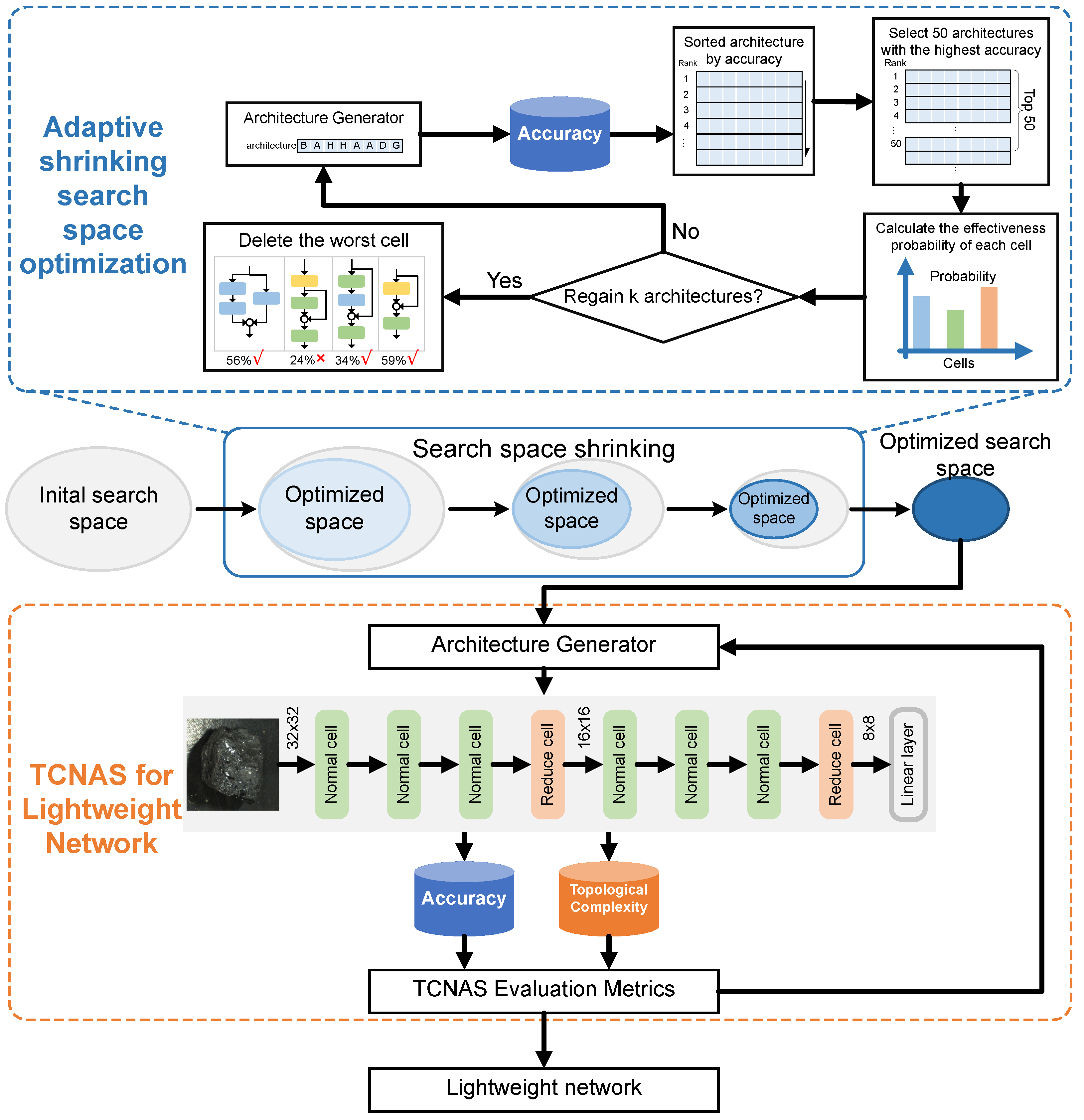
This research proposes a novel method for automatically designing lightweight neural network architectures specifically for coal and gangue classification tasks. The essence of this method lies in minimizing human intervention during the NAS process, thereby significantly enhancing the efficiency and performance of the search. The overall framework of TCNAS is shown in Figure 2.
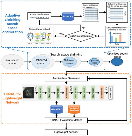
Figure 2.
Explanation of TCNAS for optimizing the search space and conducting a lightweight network search. In the first stage, the search is conducted based on accuracy as the evaluation metric to obtain the effectiveness probability of the cell and gradually eliminate cells with poor performance to optimize the search space. In the second stage, a multi-objective optimization is performed on accuracy and topological complexity in the optimized search space to guide the NAS search for a lightweight network.
The TCNAS process is divided into two phases. The first phase is dedicated to search space optimization. The aim is to explore an initial search space guided by the principle of optimal precision, gradually eliminating poorly performing units to refine the search space and avoid potential combinatorial explosions. The second phase focuses on evaluating the topology complexity of the network. Within this refined search space, the search task shifts to finding lightweight and efficient architectures. This approach not only improves the accuracy and efficiency of the search but also greatly reduces the resources required for training and deployment, providing an effective and practical solution for the automatic classification of coal and gangue.
3.1. Adaptive Shrinking Search Space Optimization Method
Traditional cell-based search spaces, which often share the best normal and reduction cells, can lead to limited global diversity in network architectures. To overcome this limitation and enhance the diversity of architectures obtained through NAS, this paper sets exclusive sub-search spaces for different network depths. This approach allows networks to be constructed in a more flexible and diverse manner. Specifically, the network adopts a chain-like structure, consisting of eight cells connected by a fully connected layer. After every three normal cells, there is a reduction cell for dimensionality reduction. Independent sub-search spaces are set for the first three normal cells, the last three normal cells, and the two reduction cells in the network. This arrangement allows each layer of the network to choose the most suitable cell from its corresponding sub-search space, and the cells between different layers can be different. Each sub-search space contains the most effective cells at the respective depth, thereby enhancing the overall performance of the network.
In the design of the search space, depthwise separable convolutions are extensively used in place of traditional convolution operations to create a more lightweight search space. In order to ensure that the search space is excellent, an adaptive shrinking search space optimization method is adopted. This approach allows human experts to design what they consider efficient cells as the initial search space based on their professional knowledge and judgment, thus avoiding excessive time spent on determining whether the search space is reasonable.
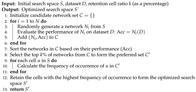
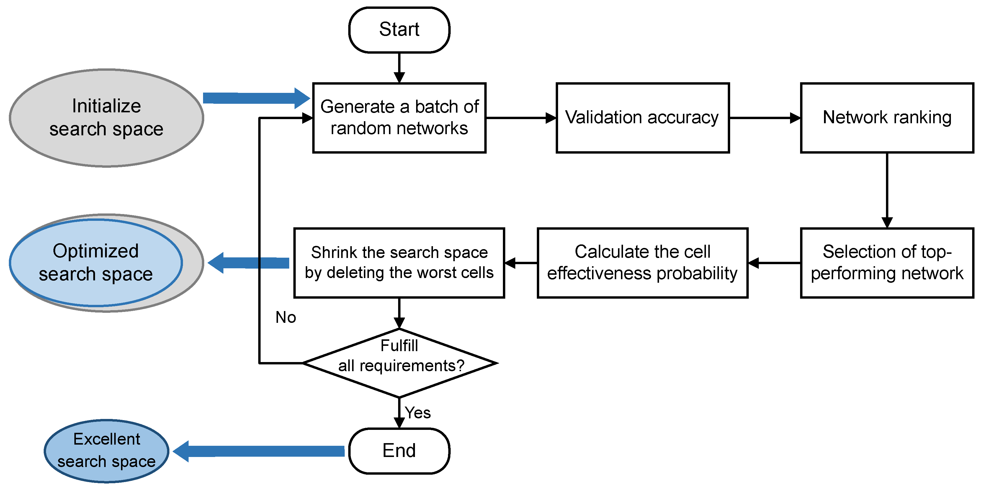
The optimization of the search space follows a structured process aimed at refining the selection of cells to improve network performance. The optimization process of the search space follows the steps of Algorithm 1: Firstly, various networks are randomly generated at the beginning of an exploration phase within a vast search space predefined by a human. Then, the performance, such as accuracy, of all generated architectures is tested and these architectures are ranked based on accuracy. Next, these architectures are ranked according to accuracy to identify the best performing architecture. A key step is to select the top k architectures and analyze how often each cell is used in all the architectures as well as in the top architectures. This analysis helps to calculate the effectiveness probability of each cell, defined as the ratio of the number of times a cell appears in top architectures to its overall usage rate. This effectiveness probability serves as a clear indicator of the cell’s contribution to improving the model performance, with higher values indicating a greater impact on improving accuracy. Subsequently, the cells with the lowest effectiveness probability are removed and those that are more effective are retained. Finally, the decision to conclude the optimization process depends on the size of the search space. If the search space has been reduced to a reasonable range, the optimization process is complete; otherwise, the process is restarted until the search space reaches an ideal size. This adaptive approach to shrinking the search space optimization can reduce labor and time costs while retaining superior units to improve search efficiency. The search space optimization process is shown in Figure 3.

Figure 3.
Flowchart of the search space optimization method for adaptive shrinkage.
The adaptive shrinking search space optimization approach is the key for TCNAS to reduce manual intervention in the field of automated architecture design. By cleverly designing and adapting the search space, TCNAS ensures that the network architecture is both diverse and efficient, allowing the system to autonomously optimize and shrink the search space within a vast and complex search domain. The method not only improves search efficiency but also facilitates the deployment of high-performance neural networks in resource-constrained environments.
| Algorithm 1 Optimize Search Space Algorithm |
 |
3.2. TCNAS Search for Lightweight Network
3.2.1. Complexity Evaluation
Based on the optimized search space, we further explore in depth how to search for lightweight networks suitable for resource-constrained environments through the TCNAS approach, maintaining a balance between efficiency and performance.
This section introduces a novel approach for evaluating the topological complexity of neural networks, drawing inspiration from Thomas McCabe’s classical complexity assessment framework [50] originally developed for computer software testing. McCabe’s methodology quantifies complexity through the analysis of a program’s control flow, employing a program flowchart or directed graph to vividly depict the flow of information within the program. It is crucial to recognize that while these program flow graphs are directed, they do not inherently constitute strongly connected graphs. To address this, McCabe’s approach integrates auxiliary lines at the program’s beginning and end, converting the flow graph into a strongly connected graph and facilitating complexity computation.
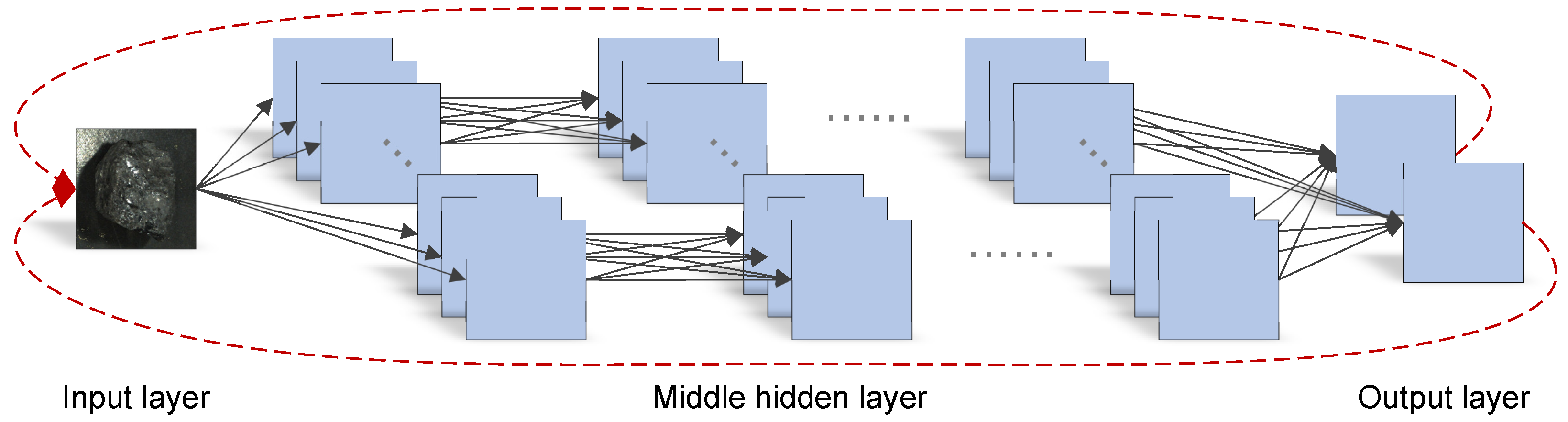
Inspired by McCabe’s method, this study proposes a new method to assess the topological complexity of neural networks. A neural network consists of multiple layers, where each node in a layer receives input from the previous layer and outputs to the next layer, up until the output layer. This process of information transfer does not involve loops, indicating that a neural network is essentially a Directed Acyclic Graph (DAG). In this research, the structural and topological information of the neural network is first converted into a format similar to a program control flow graph, and then the McCabe complexity assessment method is applied for analysis.
To accomplish this transformation, the study constructs auxiliary lines to connect the output and input layers of the neural network, as shown in Figure 4. These auxiliary lines, functioning as 1 × 1 convolutions, not only preserve the original topological structure of the neural network but also transform it into a DAG. By doing so, this study successfully applies McCabe’s complexity assessment method to the field of neural networks, providing an effective tool for understanding and analyzing the topological complexity of neural networks.
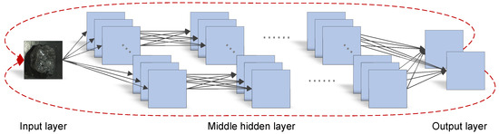
Figure 4.
Strongly connected graph of the topology of the neural network. Each node represents a feature map. Each edge represents a convolution. Assuming a 1 × 1 convolution between the output layer and the input layer, construct a directed auxiliary line from the output layer feature map to the input layer feature map to form a strongly connected graph.
When applying McCabe’s complexity assessment method to neural networks, two key aspects require special attention. First, the topological structure of the neural network must be accurately represented, which includes clearly defining the number of layers in the network, the number of feature maps in each layer, and the connections between layers. In this representation, each feature map is viewed as a node, and the convolution operations between two feature maps are represented as edges. Second, identifying the strongly connected components within the neural network architecture is necessary. The topological structure of a neural network typically forms a DAG with multiple inputs and outputs. To construct a strongly connected graph, this study achieves this by adding auxiliary lines and calculating the number of strongly connected components. In a strongly connected neural network structure, finding the largest strongly connected subgraph is a key step in determining the number of strongly connected components.
Therefore, the complexity of a neural network can be calculated based on the number of nodes, the number of edges, and the number of strongly connected components. Taking into account the influence of convolution kernels of varying sizes on the network’s computational complexity, this study assigns appropriate weight coefficients to these kernels based on their dimensions. In this method, the number of feature maps is denoted as N, the number of strongly connected components as P, and complexity weight coefficients for convolution kernels of different sizes are set as . The calculation formula for the topological complexity T of the neural network can be represented as a function that combines these parameters. This approach allows for a more precise assessment and understanding of the structural and computational complexity of neural networks, providing a new perspective for network design and optimization. The formula for calculating the topological complexity T of a neural network is as follows:
where represents the complexity weighting coefficient of the i-th layer convolution, and represents the number of edges between the i-th and (i + 1)-th layers in the strongly connected graph of the neural network topology. N represents the number of nodes, i.e., the number of feature maps in the neural network topology. P represents the number of strongly connected components in the neural network topology.
By accurately evaluating the topological complexity of networks, the performance and efficiency of network architectures can be better understood and analyzed, further driving the search for efficient and computationally inexpensive models. Concurrently, architectures that are computationally expensive with limited performance gains can be effectively identified and eliminated, thus ensuring that the search direction is focused on efficient network architectures.
3.2.2. Multi-Objective Optimization Guided Lightweight Network Search
Based on the above understanding of network complexity, this study employs a multi-objective optimization approach to guide the search of lightweight networks, aiming to find an ideal balance that satisfies performance requirements while accommodating resource constraints.
As the applications of convolutional neural networks expand and the number of network layers increases, deploying them on edge devices with limited computing resources becomes increasingly challenging. Against this backdrop, traditional NAS methods, which typically use accuracy as the sole performance metric, can identify high-accuracy networks but face challenges in practical industrial applications. Particularly on industrial devices with limited hardware resources, high-accuracy models are difficult to run and deploy effectively.
To address the challenges of model deployment in industrial applications, the search process in NAS needs to go beyond mere accuracy considerations and incorporate multiple evaluation metrics. Topological complexity becomes one of these key metrics, reflecting the complexity of the network architecture, including factors such as depth, width, and connectivity. Generally, the higher the topological complexity of a network, the more computational resources it requires. Therefore, TCNAS seeks a balance between accuracy and hardware resource utilization, making it more suitable for environments with limited computational resources.
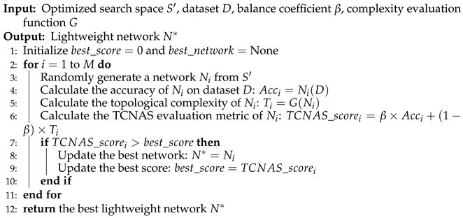
TCNAS employs a linear weighted sum approach for multi-objective optimization, aiming to find an appropriate balance between topological complexity and accuracy. It combines multiple objective functions into a comprehensive target function, namely the TCNAS evaluation metric. This enables TCNAS to search for neural networks that are both low in topological complexity and high in accuracy, allowing these networks to be effectively run and deployed on devices with limited computational resources. Multi-objective optimization guides the lightweight network search process following the steps of Algorithm 2. The calculation formula for the TCNAS evaluation metric takes into account both topological complexity and accuracy, thus providing a comprehensive assessment of network performance. The formula for calculating the TCNAS evaluation metric using topological complexity and accuracy is as follows:
where S denotes the TCNAS evaluation metric proposed in this paper, which can show the balance between accuracy and complexity of the architecture. Acc and represent the accuracy of the test set and the normalized accuracy of the test set, respectively, and T and denote the topological complexity of the neural network and its normalized form. Where is the TCNAS balance coefficient, which is the balance coefficient between accuracy and topological complexity according to the actual needs of the task, Acc represents the accuracy of the test set, and T represents the topological complexity of the neural network.
| Algorithm 2 Multi-objective Optimization Guided Lightweight Network Search |
 |
To improve model generalization, TCNAS uses L1 and L2 regularization techniques to prevent overfitting. However, excessive regularization can negatively impact model performance. Therefore, TCNAS performs hyperparameter searches on both L1 and L2 regularization coefficients during model performance evaluation; i.e., both network parameters and architecture are searched during the search process. This helps to allow further reduction of manual intervention during the architecture design process and improves the adaptive tuning capability of the system.
In essence, integrating multi-objective optimization into the TCNAS process demonstrates a commitment to designing neural networks that are both predictive and consider operational constraints. This balanced approach ensures that the networks obtained from the TCNAS process are practical and deployable solutions, reflecting the crucial principles of efficiency and effectiveness in the field of neural network applications.
4. Experiment
4.1. Data Acquisition and Development Environment
We collected over 20,000 original images from coal mining enterprises. After filtering, cropping, and labeling the coal and gangue images collected from the coal mining site, 8542 coal and gangue grey scale images were obtained as the dataset, of which 6542 were used for training, 1000 for validation, and 1000 for testing. Our coal and gangue images dataset is shown in Figure 5. We resized each image to 32 × 32.
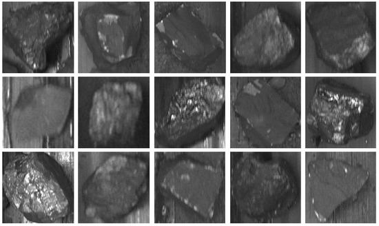
Figure 5.
Example image of our coal and gangue dataset.
These images were captured using an industrial camera equipped with a VS1614-10m. To fully consider the effects of the different speeds of motion of the conveyor belt, image acquisition was conducted at three typical speeds: low speed (0.1 m/s), medium speed (0.2 m/s), and high speed (0.4 m/s). Under these settings, the camera’s field of view was set to 80 cm × 80 cm, and the frame rate of the camera was 60 frames per second.
We used Python and PyTorch with batch normalization to implement our method. During the optimization of the search space, in order to speed up the efficiency of the multi-round search and training, we use the Adam optimizer. After the search space is optimized, in order to further improve the accuracy and convergence performance of the network, we use the SGD optimizer for search and training. In the process of training the network, we introduced L1 and L2 regularization techniques to prevent overfitting, which helps NAS to find architecture with better generalization ability. During the architectural optimization process, we also performed hyperparameter searches on the number of channels, L1 and L2 regularization coefficients, which helped to achieve the goal of avoiding overfitting while ensuring that the model was sufficiently expressive. The batch size was set to 64, and the momentum of the SGD optimizer was set to 0.9. The learning rate and weight decay coefficient were both set to 0.001. We used the warm-up strategy and the multi-step decay learning rate adjustment strategy to ensure that the model can converge quickly and stably. The learning rate was reduced to half its original value at the 10th and 18th epochs.
The proposed TCNAS method has been deployed on a Windows 10 system, with an AMD Ryzen 9 5950X 16-Core Processor (3.40 GHz), 32 GB DDR4 3600 MHz RAM, and an NVIDIA GeForce RTX 3080 Ti with 12 GB of video memory. The code was programmed with Python 3.7, PyTorch 1.8.1, cuda 11.1, and numpy 1.21.6 to develop our proposal.
4.2. Define the Initial Search Space
When defining the initial search space, we borrowed design concepts from three classic neural network architectures, Vgg [51], Resnet [52], and Mobilenet [53]. These architectures provide us with valuable references by employing different techniques to balance the expressiveness and computational cost of the network. Vgg increases the depth of the network by stacking multiple 3 × 3 convolutional layers to improve expressiveness while keeping the computational cost relatively low due to the small kernel size of the convolutions. Resnet addresses the vanishing gradient problem in deep networks by introducing skip connections, allowing for the construction of deeper network architectures. Mobilenet significantly reduces the number of parameters and computational cost by replacing traditional convolutions with depthwise separable convolutions, maintaining high accuracy levels. Building on these concepts, our search space is designed to contain 1 × 1 convolutions, 3 × 3 convolutions, and depthwise 3 × 3 convolutions for constructing each cell. The 1 × 1 convolutions are used for channel mixing to enhance the network’s non-linear expressive capability. The 3 × 3 convolutions serve as basic feature extractors, balancing performance and computational cost. The depthwise 3 × 3 convolutions, inspired by Mobilenet’s design, further reduce computational costs.
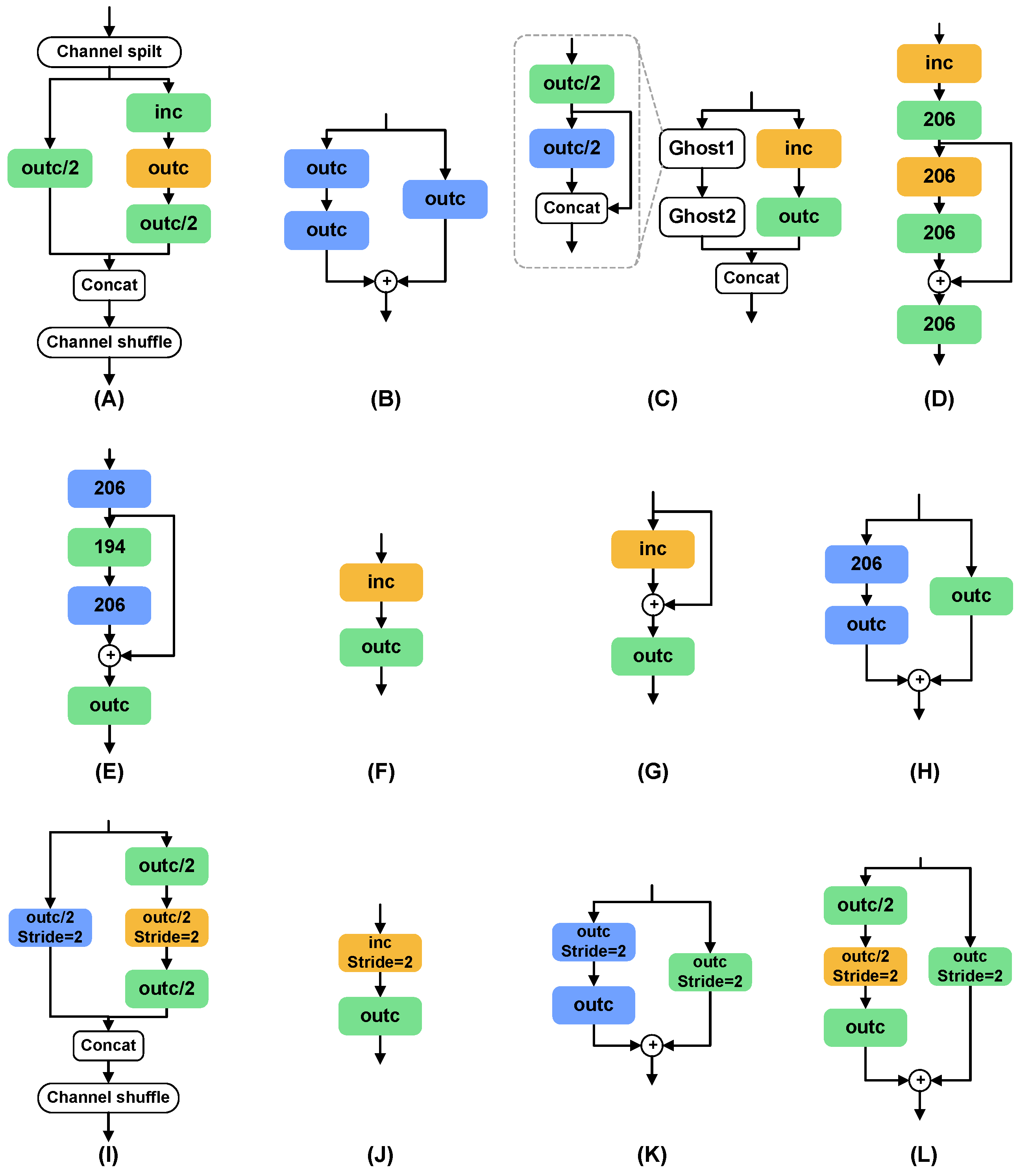
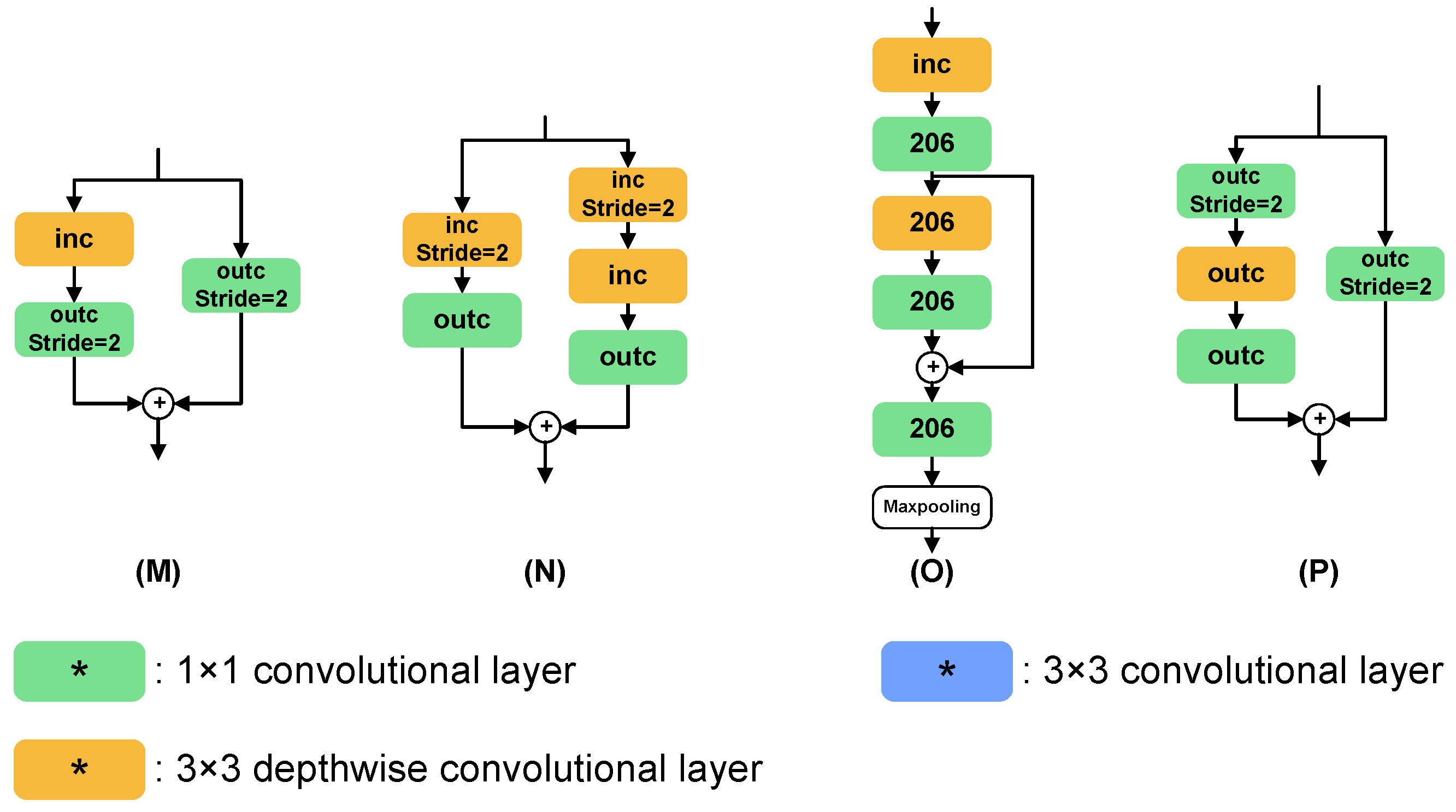
We select eight normal cells and eight reduction cells to define the initial search space, providing sufficient flexibility and diversity for the search algorithm to explore different network topologies. Normal cells are used to maintain the dimensions of the feature maps, while reduction cells halve the dimensions of the feature maps. The overall network structure consists of six normal cells and two reduction cells, with a configuration of three normal cells followed by a reduction cell, based on the best practices from multiple experiments and previous research [9,12,27]. This configuration balances the depth and width of the network and ensures sufficient representation capacity while limiting computational cost. Additionally, this grouping helps the model to capture features at different scales, enhancing the model’s adaptability to scale variations. Through the initial search space shown in Figure 6, we provide a balanced starting point for network search, aiming to find a network architecture that is both highly accurate and computationally efficient through subsequent search processes.
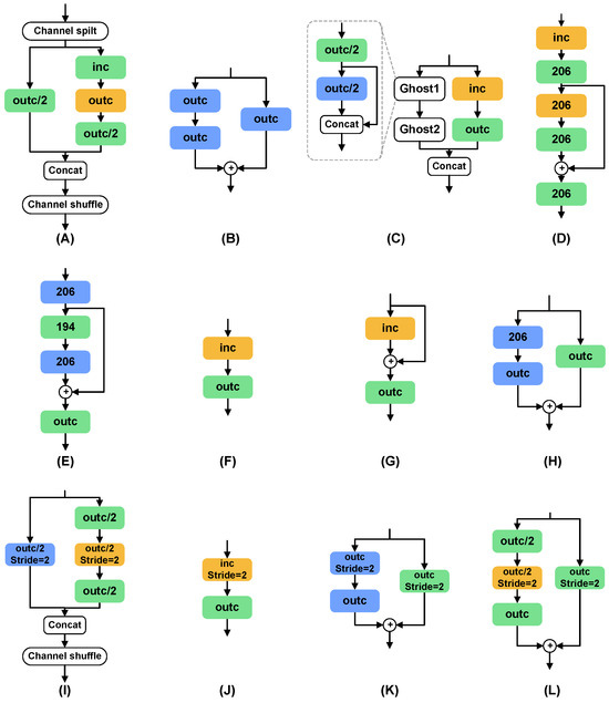
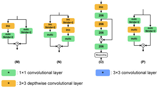
Figure 6.
The architecture of the search space. * indicates the number of output channels and stride settings for each convolutional layer. (A–H) indicate normal cells, and (I–P) indicate reduction cells. Reduction cells are mainly downsampled by the stride of 2 and maxpooling.
4.3. Search Space Optimization Results
The proposed search space adaptive optimization and reduction method is evaluated based on accuracy as the only performance metric for searching and is searched for a total of 500 architectures. The ratio of the number of times the cell is used in the 50 networks with the best performance to the number of times the cell is used in all generated networks is used to calculate the effectiveness probability of each cell. After optimization, the effectiveness probabilities of each cell are shown in Table 3. The four most effective cells with the highest effectiveness probability are selected to form the optimized search space for each sub-search space. In the first three layers of normal cells, the most effective cells are H, G, A, and E, with effectiveness probabilities of 0.245, 0.242, 0.223, and 0.206, respectively. In the last three layers of normal cells, the most effective cells are F, G, B, and C, with effectiveness probabilities of 0.247, 0.242, 0.222, and 0.216, respectively. The most effective cells of the two-layer reduction cell are O, M, I, and K, with effectiveness probabilities of 0.339, 0.268, 0.241, and 0.210, respectively. After the search space is optimized, an empty operation cell is added to the optimized normal cell search space, which allows the NAS to have the ability to adaptively adjust the network layer depth during the next stage of TCNAS search for lightweight architectures, which helps discover networks with fewer layers and lower architectural complexity.
Table 3.
The effectiveness probability of each cell after pre-search.
4.4. Compare the Ratio of Parameters between Various Convolutions
Before conducting TCNAS, it is necessary to determine the ratio between the various convolutional computation costs. Therefore, we conducted experimental comparisons of two mainstream neural networks, Vgg and Resnet. The architectures used in this experiment only include commonly used 1 × 1, 3 × 3, and 3 × 3 depthwise convolutions. It is worth noting that the number of parameters in the 3 × 3 convolution is a multiple of the number of groups in the 3 × 3 depthwise convolution. Therefore, once the number of parameters in a 3 × 3 convolution is known, the number of parameters in a 3 × 3 depthwise convolution can be determined. We measured the number of parameters in four network architectures by replacing the convolutional layers with all 1 × 1 convolutions and all 3 × 3 convolutions. We replace all the convolutions in the four networks with 1 × 1 convolutions or 3 × 3 convolutions and then calculate the parameters of these networks to approximate the computational cost of 3 × 3 convolutions and 1 × 1 convolutions. The experimental results in Table 4 show that the total number of parameters in a network consisting entirely of 3 × 3 convolutions is about eight times that of a network consisting entirely of 1 × 1 convolutions. Therefore, the ratio of computational costs between 1 × 1, 3 × 3, and 3 × 3 depthwise convolutions is . This ratio will be used as the weight ratio of each convolution to calculate the topological complexity of the neural network in the following experiments.
Table 4.
Comparison of the parameters of the above four networks all constructed by 1 × 1 or 3 × 3 convolutions, where ‘parameter scale’ is the parameters of the network constructed by all 3 × 3 convolutions divided by the parameters of the network constructed by all 1 × 1 convolutions.
4.5. TCNAS Balance Coefficient Value Experiment
In the TCNAS search method for lightweight networks proposed in this paper, the accuracy and topological complexity of the model are given different weights. Then they are linearly weighted and summed. In this process, the selection of weights is crucial, effectively achieving a suitable balance between accuracy and topology complexity. We selected TCNAS balance coefficient to be 0.5, 0.6, 0.7, and 0.8 to conduct TCNAS search experiments. Search under different values, and take the average performance indicators of the six architectures with the largest TCNAS evaluation metric obtained from the search. The experimental results are shown in Table 5. When is 0.5, although the number of parameters and topological complexity is low, its accuracy is also relatively low. On the contrary, when is 0.8, although the accuracy is higher, it requires more parameters and has a larger topological complexity. This experiment determined that a of 0.6 is a more appropriate weight distribution scheme. The following experiments will use 0.6 as the TCNAS balance coefficient for further experimental verification.
Table 5.
The results of various performance indicators of the excellent network obtained by searching under different TCNAS balance coefficients.
4.6. Comparison with Other Hardware Cost Metric Search Methods
To validate the effectiveness of the proposed method for evaluating topological complexity, we used three hardware cost indicators: parameter, latency, and topological complexity. Each of the three hardware cost metrics is fused with accuracy for three lightweight architecture search experiments. Our proposed TCNAS performs a lightweight architecture search guided by both topological complexity and accuracy and compares search results using parameter count and latency as measures of computation cost. The latency refers to the real hardware inference time on a 3080 Ti GPU in the workstation of the author. The previous experiments have verified that the TCNAS balance coefficient of 0.6 is a suitable parameter, so the accuracy and topology complexity are fused at a ratio of 6:4. The number of parameters and latency are experimented at the corresponding suitable ratios.
In the optimized search space, we used three hardware cost metrics and accuracy to guide the search for 500 architectures. We compare the performance of the five architectures with the best overall performance in the experiments of different hardware cost indicators. Table 6 and Table 7 show the results of experiments conducted using parameter and latency as hardware cost metrics, respectively. Although the first-ranked architecture is 0.1% less accurate than the second-ranked architecture, the parameters are only 0.5 times those of the second-ranked architecture, which has the best comprehensive performance.
Table 6.
Performance of the architecture obtained from the search guided by accuracy and parameters.
Table 7.
Performance of the architecture obtained from the search guided by accuracy and latency.
The top five architectures obtained from the TCNAS are shown in Table 8. TCNAS performs multi-objective optimization on accuracy and topology complexity, and searches for the architecture with the best overall performance [Q, G, Q, I, F, Q, B, O, 192, 32, 96, 128, 96, 64, 32, 64, 64], which achieved the highest accuracy rate of 83.3%, a topology complexity of 155,487, and a TCNAS evaluation metric of 0.8883. Our experimental results demonstrate that the proposed topological complexity metric can effectively reflect the complexity level of neural networks.
Table 8.
Performance of the architecture obtained by TCNAS.
4.7. Performance Comparison with Other NAS Methods
In this experiment, we evaluated the performance of different cell-based NAS methods under the same 100 h of search time cost and found that TCNAS has significant advantages in adaptive shrinking search space optimization and multi-objective optimization. Table 9 compares the search cost, top-1 accuracy, parameters, and topological complexity of ProxylessNAS, DARTS, ENAS, NASNet, and our TCNAS.
Table 9.
Performance comparison of cell-based NAS methods under the same search condition for 100 h.
ProxylessNAS, despite using parameter sharing and random uniform sampling to reduce the search space, did not use a proxy model during the search process, resulting in relatively high search cost, parameters, and topological complexity of 4.71 M and 97.7 M, respectively. DARTS and ENAS, while achieving higher accuracy, had relatively large parameters and topological complexity of 4.38 M/91.8 M and 3.92 M/82.1 M, respectively. NASNet adopted a multi-objective optimization strategy, significantly reducing the parameter count to 0.79 M while maintaining a top-1 accuracy of 80.23%. However, the topological complexity remained relatively high.
However, our TCNAS demonstrated unique advantages in adaptive shrinking search space optimization and multi-objective optimization. By treating parameters and topological complexity as one of the objectives in multi-objective optimization, we achieved an impressive 83.3% top-1 accuracy with only 0.17 M parameters. This is a dual-target optimization of high accuracy and low parameters that other methods have failed to achieve. At the same time, TCNAS also showed significant advantages in topological complexity, reducing it to just 4.0 M compared to other methods. This means that our TCNAS method can find more efficient neural network architectures, achieving a better balance between accuracy and model complexity.
In summary, TCNAS has successfully achieved high accuracy, low parameters, and low topological complexity through the combined effects of adaptive shrinking of the search space and multi-objective optimization. This makes TCNAS a promising method with the potential to enable efficient neural network design in resource-constrained conditions.
4.8. Performance Comparison with Other Networks
To validate the network performance obtained by TCNAS search, we tested our method on coal and gangue image datasets. We compared the performance of the optimized networks obtained by TCNAS with mainstream networks, lightweight networks, and specialized networks for coal and gangue classification [9], including accuracy, F1-score, and recall metrics, as shown in Table 10. Recall is a metric that evaluates the ability of the model to identify positive class samples, which can reflect the ability of the model to capture positive samples. F1-score is the reconciled average of accuracy and recall, a balanced metric of accuracy and recall. The results show that the optimal architecture searched by TCNAS achieves the highest accuracy of 83.3%, which is higher than Cellnet40 [9], the network with the highest classification accuracy of coal and gangue in the past, and has only 1/53 the number of parameters as Cellnet40. Compared with mainstream networks and lightweight networks, TCNAS not only achieves higher accuracy but also excels in F1-score and recall, while maintaining a lower number of parameters, achieving the optimal balance between accuracy and efficiency. Experiments show that TCNAS, combined with topology complexity, can effectively automatically search and design a network with higher accuracy and simpler architecture. This is of great significance for deploying and promoting deep neural networks in the industrial field.
Table 10.
Comparison of the performance of TCNAS optimal network with mainstream network and lightweight network on coal and gangue classification dataset.
5. Discussion
From a topological perspective, this is a relatively unexplored area in the study of neural networks. We made an early attempt to evaluate the complexity of neural networks by quantifying the number of nodes and edges. Different from traditional NAS, which focuses on hardware metrics (e.g., Flops and latency), TCNAS directly quantifies the complexity and computational cost of a network by evaluating the number of nodes and edges inside the network. This approach not only strengthens the association between network complexity and computational cost but also proves to be efficient in searching for lightweight networks.
In this study, TCNAS successfully introduced the concept of topological complexity in the NAS domain, demonstrating that utilizing this metric can effectively search for networks that are structurally simple and have low computational costs. Although these networks are not always the highest accuracy, they train quickly, help prevent overfitting, and are more suitable for deployment in environments with limited computational resources, thus promoting the understandability and interpretability of the neural network. Compared to the work of Cellnet40, our method can reduce the number of network parameters by up to 53 times, further demonstrating the ability of TCNAS to find lightweight and efficient networks. Additionally, we introduced an adaptive shrinking search space optimization method to improve search efficiency. This method allows for the automatic selection of the best cells designed by human experts based on intuition as the optimized search space, thereby reducing the degree of human intervention and decreasing design time and labor costs.
TCNAS demonstrates significant potential and flexibility in handling diverse architectures and optimizing search algorithms. The approach is not only suitable for specific tasks, such as coal and gangue classification, but its design philosophy and implementation mechanism enable it to be easily extended to other domains, such as semantic segmentation and other image recognition tasks. In particular, we note that the attention module has a significant effect on accuracy improvement, and TCNAS can flexibly incorporate advanced architectures like an attention module into the search space as needed to meet diverse requirements.
Limitations: Despite the exceptional performance demonstrated by TCNAS in various aspects, we recognize that it has some limitations. Particularly, regarding the adaptive shrinking method for search space optimization, the process reduces human intervention but still requires some human intervention and involvement, especially during the design phase of the initial search space. There is a gap between this need for human involvement and the ultimate goal of AutoML, which aims to eliminate the need for human intervention.
To get closer to the ultimate goal of AutoML, future research will focus on reducing human intervention. In search space design and optimization, the aim is to achieve full automation of search space construction as well as automated design of high-level architectures. By introducing topological complexity at an earlier stage and imposing complexity constraints on the cell structure, it will help to reduce invalid searches, improve search efficiency, and facilitate the development of the automated design of lightweight networks.
6. Conclusions
This paper proposes the TCNAS method, which innovatively integrates topology complexity assessment and adaptive search space optimization to address the challenging issue of efficiently running high-precision networks on industrial devices with limited computational resources. Overall, the proposed TCNAS method offers a promising solution to the challenges of light weight and self-adjustment in deep neural networks. By integrating topological complexity evaluation and efficient search techniques, it enables the automated discovery of lightweight networks that maintain high accuracy, making it particularly suitable for industrial applications. Compared with mainstream networks and lightweight networks, the optimal network searched by TCNAS has higher accuracy, simpler structure, and fewer parameters. The optimal architecture searched by TCNAS achieved an accuracy of 83.3% in the coal and gangue classification experiment, which is 1.5% higher than the accuracy of the best network, Cellnet40, in this task, previously achieved by the author team, but with about 53 times fewer parameters than Cellnet40. Therefore, the experiment effectively verifies that the topological complexity evaluation method we proposed provides a new idea for lightweight neural network research.
Although TCNAS performs well in many aspects, it still has some limitations. In particular, in the adaptive reduced search space optimization approach, this process reduces manual intervention but still requires manual involvement in the initial design phase. Future research will aim to further reduce manual intervention and automate search space construction and efficient design.
Author Contributions
Conceptualization, W.Z. and Y.H.; methodology, W.Z. and Y.H.; software, Y.H.; validation, Y.H. and H.L.; formal analysis, H.L., Z.Z. (Zhongbo Zhang) and W.F.; investigation, Z.Z. (Zhengjun Zhu); resources, Y.H.; data curation, H.L.; writing—original draft preparation, W.Z. and Y.H.; writing—review and editing, W.Z., Y.H. and H.L.; project administration, W.Z. and W.-C.Y.; funding acquisition, W.Z. and H.L. All authors have read and agreed to the published version of the manuscript.
Funding
This research is supported by the Guangdong Key Project (2021B0101410002), and National Natural Science Foundation of China (62106048).
Data Availability Statement
Due to the nature of this research, participants in this study did not agree for their data to be shared publicly, so supporting data is not available.
Conflicts of Interest
Zhengjun Zhu was employed by China Coal Technology Engineering Group Tangshan Research Institute. The authors declare that they have no known competing financial interests or personal relationships that could have appeared to influence the work reported in this paper.
References
- Lai, W.; Zhou, M.; Hu, F.; Bian, K.; Song, H. A study of multispectral technology and two-dimension autoencoder for coal and gangue recognition. IEEE Access 2020, 8, 61834–61843. [Google Scholar] [CrossRef]
- Dou, D.; Zhou, D.; Yang, J.; Zhang, Y. Coal and gangue recognition under four operating conditions by using image analysis and Relief-SVM. Int. J. Coal Prep. Util. 2018, 40, 473–482. [Google Scholar] [CrossRef]
- Hou, W. Identification of coal and gangue by feed-forward neural network based on data analysis. Int. J. Coal Prep. Util. 2019, 39, 33–43. [Google Scholar] [CrossRef]
- Eshaq, R.M.A.; Hu, E.; Li, M.; Alfarzaeai, M.S. Separation between coal and gangue based on infrared radiation and visual extraction of the YCbCr color space. IEEE Access 2020, 8, 55204–55220. [Google Scholar] [CrossRef]
- Hu, F.; Zhou, M.; Yan, P.; Liang, Z.; Li, M. A Bayesian optimal convolutional neural network approach for classification of coal and gangue with multispectral imaging. Opt. Lasers Eng. 2022, 156, 107081. [Google Scholar] [CrossRef]
- Lv, Z.; Wang, W.; Xu, Z.; Zhang, K.; Fan, Y.; Song, Y. Fine-grained object detection method using attention mechanism and its application in coal–gangue detection. Appl. Soft Comput. 2021, 113, 107891. [Google Scholar] [CrossRef]
- Pu, Y.; Apel, D.B.; Szmigiel, A.; Chen, J. Image recognition of coal and coal gangue using a convolutional neural network and transfer learning. Energies 2019, 12, 1735. [Google Scholar] [CrossRef]
- Lv, Z.; Wang, W.; Xu, Z.; Zhang, K.; Lv, H. Cascade network for detection of coal and gangue in the production context. Powder Technol. 2021, 377, 361–371. [Google Scholar] [CrossRef]
- Sun, L.; Zhu, W.; Lu, Q.; Li, A.; Luo, L.; Chen, J.; Wang, J. CellNet: An Improved Neural Architecture Search Method for Coal and Gangue Classification. In Proceedings of the 2021 International Joint Conference on Neural Networks (IJCNN), Shenzhen, China, 18–22 July 2021; pp. 1–9. [Google Scholar]
- Liu, Q.; Li, J.; Li, Y.; Gao, M. Recognition methods for coal and coal gangue based on deep learning. IEEE Access 2021, 9, 77599–77610. [Google Scholar] [CrossRef]
- Zoph, B.; Le, Q.V. Neural architecture search with reinforcement learning. arXiv 2016, arXiv:1611.01578. [Google Scholar]
- Zoph, B.; Vasudevan, V.; Shlens, J.; Le, Q.V. Learning transferable architectures for scalable image recognition. In Proceedings of the IEEE Conference on Computer Vision and Pattern Recognition, Salt Lake City, UT, USA, 18–23 June 2018; pp. 8697–8710. [Google Scholar]
- Real, E.; Aggarwal, A.; Huang, Y.; Le, Q.V. Regularized evolution for image classifier architecture search. In Proceedings of the AAAI Conference on Artificial Intelligence, Honolulu, HI, USA, 27 January–1 February 2019; Volume 33, pp. 4780–4789. [Google Scholar]
- Peng, H.; Du, H.; Yu, H.; Li, Q.; Liao, J.; Fu, J. Cream of the crop: Distilling prioritized paths for one-shot neural architecture search. Adv. Neural Inf. Process. Syst. 2020, 33, 17955–17964. [Google Scholar]
- Wu, J.; Kuang, H.; Lu, Q.; Lin, Z.; Shi, Q.; Liu, X.; Zhu, X. M-FasterSeg: An efficient semantic segmentation network based on neural architecture search. Eng. Appl. Artif. Intell. 2022, 113, 104962. [Google Scholar] [CrossRef]
- Ghiasi, G.; Lin, T.Y.; Le, Q.V. Nas-fpn: Learning scalable feature pyramid architecture for object detection. In Proceedings of the IEEE/CVF Conference on Computer Vision and Pattern Recognition, Long Beach, CA, USA, 15–20 June 2019; pp. 7036–7045. [Google Scholar]
- Liu, C.; Chen, L.C.; Schroff, F.; Adam, H.; Hua, W.; Yuille, A.L.; Fei-Fei, L. Auto-deeplab: Hierarchical neural architecture search for semantic image segmentation. In Proceedings of the IEEE/CVF Conference on Computer Vision and Pattern Recognition, Long Beach, CA, USA, 15–20 June 2019; pp. 82–92. [Google Scholar]
- Chen, Y.; Yang, T.; Zhang, X.; Meng, G.; Xiao, X.; Sun, J. Detnas: Backbone search for object detection. Adv. Neural Inf. Process. Syst. 2019, 32, 6642–6652. [Google Scholar]
- Luo, R.; Tan, X.; Wang, R.; Qin, T.; Li, J.; Zhao, S.; Chen, E.; Liu, T.Y. Lightspeech: Lightweight and fast text to speech with neural architecture search. In Proceedings of the ICASSP 2021—2021 IEEE International Conference on Acoustics, Speech and Signal Processing (ICASSP), Toronto, ON, Canada, 6–11 June 2021; pp. 5699–5703. [Google Scholar]
- Lee, J.H.; Chang, J.H.; Yang, J.M.; Moon, H.G. NAS-TasNet: Neural Architecture Search for Time-Domain Speech Separation. IEEE Access 2022, 10, 56031–56043. [Google Scholar] [CrossRef]
- Klyuchnikov, N.; Trofimov, I.; Artemova, E.; Salnikov, M.; Fedorov, M.; Filippov, A.; Burnaev, E. Nas-bench-nlp: Neural architecture search benchmark for natural language processing. IEEE Access 2022, 10, 45736–45747. [Google Scholar] [CrossRef]
- Li, Y.; Hao, C.; Li, P.; Xiong, J.; Chen, D. Generic neural architecture search via regression. Adv. Neural Inf. Process. Syst. 2021, 34, 20476–20490. [Google Scholar]
- Benmeziane, H.; Maghraoui, K.E.; Ouarnoughi, H.; Niar, S.; Wistuba, M.; Wang, N. A comprehensive survey on hardware-aware neural architecture search. arXiv 2021, arXiv:2101.09336. [Google Scholar]
- Raja, K.C.; Kannimuthu, S. Conditional Generative Adversarial Network Approach for Autism Prediction. Comput. Syst. Sci. Eng. 2023, 44, 742–755. [Google Scholar]
- Zhu, W.; Yeh, W.; Chen, J.; Chen, D.; Li, A.; Lin, Y. Evolutionary convolutional neural networks using abc. In Proceedings of the 2019 11th International Conference on Machine Learning and Computing, Zhuhai, China, 22–24 February 2019; pp. 156–162. [Google Scholar]
- Ang, K.M.; Lim, W.H.; Tiang, S.S.; Sharma, A.; Towfek, S.; Abdelhamid, A.A.; Alharbi, A.H.; Khafaga, D.S. MTLBORKS-CNN: An Innovative Approach for Automated Convolutional Neural Network Design for Image Classification. Mathematics 2023, 11, 4115. [Google Scholar] [CrossRef]
- Liu, H.; Simonyan, K.; Yang, Y. Darts: Differentiable architecture search. arXiv 2018, arXiv:1806.09055. [Google Scholar]
- Guo, Y.; Chen, Y.; Zheng, Y.; Zhao, P.; Chen, J.; Huang, J.; Tan, M. Breaking the curse of space explosion: Towards efficient nas with curriculum search. In Proceedings of the International Conference on Machine Learning. PMLR, Virtual, 13–18 July 2020; pp. 3822–3831. [Google Scholar]
- Zhou, D.; Jin, X.; Lian, X.; Yang, L.; Xue, Y.; Hou, Q.; Feng, J. AutoSpace: Neural Architecture Search with Less Human Interference. In Proceedings of the IEEE/CVF International Conference on Computer Vision, Montreal, BC, Canada, 11–17 October 2021; pp. 337–346. [Google Scholar]
- Huang, J.; Xue, B.; Sun, Y.; Zhang, M.; Yen, G.G. Split-Level Evolutionary Neural Architecture Search With Elite Weight Inheritance. IEEE Trans. Neural Netw. Learn. Syst. 2023. [Google Scholar] [CrossRef]
- Vidnerová, P.; Kalina, J. Multi-objective Bayesian Optimization for Neural Architecture Search. In Proceedings of the Artificial Intelligence and Soft Computing: 21st International Conference, ICAISC 2022, Zakopane, Poland, 19–23 June 2022; Proceedings, Part I. Springer: Berlin/Heidelberg, Germany, 2023; pp. 144–153. [Google Scholar]
- Pham, H.; Guan, M.; Zoph, B.; Le, Q.; Dean, J. Efficient neural architecture search via parameters sharing. In Proceedings of the International Conference on Machine Learning, PMLR, Stockholm, Sweden, 10–15 July 2018; pp. 4095–4104. [Google Scholar]
- Zhang, X.; Xu, H.; Mo, H.; Tan, J.; Yang, C.; Wang, L.; Ren, W. Dcnas: Densely connected neural architecture search for semantic image segmentation. In Proceedings of the IEEE/CVF Conference on Computer Vision and Pattern Recognition, Nashville, TN, USA, 20–25 June 2021; pp. 13956–13967. [Google Scholar]
- Liu, C.; Zoph, B.; Neumann, M.; Shlens, J.; Hua, W.; Li, L.J.; Fei-Fei, L.; Yuille, A.; Huang, J.; Murphy, K. Progressive neural architecture search. In Proceedings of the European Conference on Computer Vision (ECCV), Munich, Germany, 8–14 September 2018; pp. 19–34. [Google Scholar]
- Shi, C.; Hao, Y.; Li, G.; Xu, S. EBNAS: Efficient binary network design for image classification via neural architecture search. Eng. Appl. Artif. Intell. 2023, 120, 105845. [Google Scholar] [CrossRef]
- Jin, H.; Song, Q.; Hu, X. Efficient neural architecture search with network morphism. arXiv 2018, arXiv:1806.10282. [Google Scholar]
- Yu, Z.; Bouganis, C.S. SVD-NAS: Coupling Low-Rank Approximation and Neural Architecture Search. In Proceedings of the IEEE/CVF Winter Conference on Applications of Computer Vision, Waikoloa, HI, USA, 2–7 January 2023; pp. 1503–1512. [Google Scholar]
- Tan, M.; Chen, B.; Pang, R.; Vasudevan, V.; Sandler, M.; Howard, A.; Le, Q.V. Mnasnet: Platform-aware neural architecture search for mobile. In Proceedings of the IEEE/CVF Conference on Computer Vision and Pattern Recognition, Long Beach, CA, USA, 16–17 June 2019; pp. 2820–2828. [Google Scholar]
- Zhang, L.L.; Yang, Y.; Jiang, Y.; Zhu, W.; Liu, Y. Fast hardware-aware neural architecture search. In Proceedings of the IEEE/CVF Conference on Computer Vision and Pattern Recognition Workshops, Seattle, WA, USA, 13–19 June 2020; pp. 692–693. [Google Scholar]
- Marchisio, A.; Massa, A.; Mrazek, V.; Bussolino, B.; Martina, M.; Shafique, M. NASCaps: A framework for neural architecture search to optimize the accuracy and hardware efficiency of convolutional capsule networks. In Proceedings of the 39th International Conference on Computer-Aided Design, Virtual Event, 2–5 November 2020; pp. 1–9. [Google Scholar]
- Smithson, S.C.; Yang, G.; Gross, W.J.; Meyer, B.H. Neural networks designing neural networks: Multi-objective hyper-parameter optimization. In Proceedings of the 2016 IEEE/ACM International Conference on Computer-Aided Design (ICCAD), Austin, TX, USA, 7–10 November 2016; pp. 1–8. [Google Scholar]
- Wu, B.; Dai, X.; Zhang, P.; Wang, Y.; Sun, F.; Wu, Y.; Tian, Y.; Vajda, P.; Jia, Y.; Keutzer, K. Fbnet: Hardware-aware efficient convnet design via differentiable neural architecture search. In Proceedings of the IEEE/CVF Conference on Computer Vision and Pattern Recognition, Long Beach, CA, USA, 15–20 June 2019; pp. 10734–10742. [Google Scholar]
- Cai, H.; Zhu, L.; Han, S. Proxylessnas: Direct neural architecture search on target task and hardware. arXiv 2018, arXiv:1812.00332. [Google Scholar]
- Stamoulis, D.; Ding, R.; Wang, D.; Lymberopoulos, D.; Priyantha, B.; Liu, J.; Marculescu, D. Single-path nas: Designing hardware-efficient convnets in less than 4 hours. In Proceedings of the Joint European Conference on Machine Learning and Knowledge Discovery in Databases, Würzburg, Germany, 16–20 September 2019; pp. 481–497. [Google Scholar]
- Dai, X.; Zhang, P.; Wu, B.; Yin, H.; Sun, F.; Wang, Y.; Dukhan, M.; Hu, Y.; Wu, Y.; Jia, Y.; et al. Chamnet: Towards efficient network design through platform-aware model adaptation. In Proceedings of the IEEE/CVF Conference on Computer Vision and Pattern Recognition, Long Beach, CA, USA, 15–20 June 2019; pp. 11398–11407. [Google Scholar]
- Srinivas, S.V.K.; Nair, H.; Vidyasagar, V. Hardware aware neural network architectures using FbNet. arXiv 2019, arXiv:1906.07214. [Google Scholar]
- Yang, T.J.; Howard, A.; Chen, B.; Zhang, X.; Go, A.; Sandler, M.; Sze, V.; Adam, H. Netadapt: Platform-aware neural network adaptation for mobile applications. In Proceedings of the European Conference on Computer Vision (ECCV), Munich, Germany, 8–14 September 2018; pp. 285–300. [Google Scholar]
- Zhang, X.; Jiang, W.; Shi, Y.; Hu, J. When neural architecture search meets hardware implementation: From hardware awareness to co-design. In Proceedings of the 2019 IEEE Computer Society Annual Symposium on VLSI (ISVLSI), Miami, FL, USA, 15–17 July 2019; pp. 25–30. [Google Scholar]
- Dudziak, L.; Chau, T.; Abdelfattah, M.; Lee, R.; Kim, H.; Lane, N. Brp-nas: Prediction-based nas using gcns. Adv. Neural Inf. Process. Syst. 2020, 33, 10480–10490. [Google Scholar]
- McCabe, T.J. A complexity measure. IEEE Trans. Softw. Eng. 1976, 4, 308–320. [Google Scholar] [CrossRef]
- Simonyan, K.; Zisserman, A. Very deep convolutional networks for large-scale image recognition. arXiv 2014, arXiv:1409.1556. [Google Scholar]
- He, K.; Zhang, X.; Ren, S.; Sun, J. Deep residual learning for image recognition. In Proceedings of the IEEE Conference on Computer Vision and Pattern Recognition, Las Vegas, NV, USA, 27–30 June 2016; pp. 770–778. [Google Scholar]
- Howard, A.G.; Zhu, M.; Chen, B.; Kalenichenko, D.; Wang, W.; Weyand, T.; Andreetto, M.; Adam, H. Mobilenets: Efficient convolutional neural networks for mobile vision applications. arXiv 2017, arXiv:1704.04861. [Google Scholar]
- Krizhevsky, A.; Sutskever, I.; Hinton, G.E. Imagenet classification with deep convolutional neural networks. Commun. ACM 2017, 60, 84–90. [Google Scholar] [CrossRef]
- Huang, G.; Liu, Z.; Van Der Maaten, L.; Weinberger, K.Q. Densely connected convolutional networks. In Proceedings of the IEEE Conference on Computer Vision and Pattern Recognition, Honolulu, HI, USA, 21–26 July 2017; pp. 4700–4708. [Google Scholar]
- Dosovitskiy, A.; Beyer, L.; Kolesnikov, A.; Weissenborn, D.; Zhai, X.; Unterthiner, T.; Dehghani, M.; Minderer, M.; Heigold, G.; Gelly, S.; et al. An image is worth 16x16 words: Transformers for image recognition at scale. arXiv 2020, arXiv:2010.11929. [Google Scholar]
- Zhang, X.; Zhou, X.; Lin, M.; Sun, J. Shufflenet: An extremely efficient convolutional neural network for mobile devices. In Proceedings of the IEEE Conference on Computer Vision and Pattern Recognition, Salt Lake City, UT, USA, 28–23 June 2018; pp. 6848–6856. [Google Scholar]
- Szegedy, C.; Vanhoucke, V.; Ioffe, S.; Shlens, J.; Wojna, Z. Rethinking the inception architecture for computer vision. In Proceedings of the IEEE Conference on Computer Vision and Pattern Recognition, Las Vegas, NV, USA, 26 June–1 July 2016; pp. 2818–2826. [Google Scholar]
- Chollet, F. Xception: Deep learning with depthwise separable convolutions. In Proceedings of the IEEE Conference on Computer Vision and Pattern Recognition, Honolulu, HI, USA, 21–26 July 2017; pp. 1251–1258. [Google Scholar]
- Iandola, F.N.; Han, S.; Moskewicz, M.W.; Ashraf, K.; Dally, W.J.; Keutzer, K. SqueezeNet: AlexNet-level accuracy with 50x fewer parameters and <0.5 MB model size. arXiv 2016, arXiv:1602.07360. [Google Scholar]
- Han, K.; Wang, Y.; Tian, Q.; Guo, J.; Xu, C.; Xu, C. Ghostnet: More features from cheap operations. In Proceedings of the IEEE/CVF Conference on Computer Vision and Pattern Recognition, Seattle, WA, USA, 13–19 June 2020; pp. 1580–1589. [Google Scholar]
- Ma, H.; Xia, X.; Wang, X.; Xiao, X.; Li, J.; Zheng, M. MoCoViT: Mobile Convolutional Vision Transformer. arXiv 2022, arXiv:2205.12635. [Google Scholar]

Disclaimer/Publisher’s Note: The statements, opinions and data contained in all publications are solely those of the individual author(s) and contributor(s) and not of MDPI and/or the editor(s). MDPI and/or the editor(s) disclaim responsibility for any injury to people or property resulting from any ideas, methods, instructions or products referred to in the content. |
© 2024 by the authors. Licensee MDPI, Basel, Switzerland. This article is an open access article distributed under the terms and conditions of the Creative Commons Attribution (CC BY) license (https://creativecommons.org/licenses/by/4.0/).