Time Series Prediction Based on Multi-Scale Feature Extraction

Abstract

Time series data are prevalent in the real world, particularly playing a crucial role in key domains such as meteorology, electricity, and finance. Comprising observations at historical time points, these data, when subjected to in-depth analysis and modeling, enable researchers to predict future trends and patterns, providing support for decision making. In current research, especially in the analysis of long time series, effectively extracting and integrating long-term dependencies with short-term features remains a significant challenge. Long-term dependencies refer to the correlation between data points spaced far apart in a time series, while short-term features focus on more recent changes. Understanding and combining these two features correctly are crucial for constructing accurate and reliable predictive models. To efficiently extract and integrate long-term dependencies and short-term features in long time series, this paper proposes a pyramid attention structure model based on multi-scale feature extraction, referred to as the MSFformer model. Initially, a coarser-scale construction module is designed to obtain coarse-grained information. A pyramid data structure is constructed through feature convolution, with the bottom layer representing the original data and each subsequent layer containing feature information extracted across different time step lengths. As a result, nodes higher up in the pyramid integrate information from more time points, such as every Monday or the beginning of each month, while nodes lower down retain their individual information. Additionally, a Skip-PAM is introduced, where a node only calculates attention with its neighboring nodes, parent node, and child nodes, effectively reducing the model’s time complexity to some extent. Notably, the child nodes refer to nodes selected from the next layer by skipping specific time steps. In this study, we not only propose an innovative time series prediction model but also validate the effectiveness of these methods through a series of comprehensive experiments. To comprehensively evaluate the performance of the designed model, we conducted comparative experiments with baseline models, ablation experiments, and hyperparameter studies. The experimental results demonstrate that the MSFformer model improves by 35.87% and 42.6% on the MAE and MSE indicators, respectively, compared to traditional Transformer models. These results highlight the outstanding performance of our proposed deep learning model in handling complex time series data, particularly in capturing long-term dependencies and integrating short-term features.

1. Introduction

Time series consists of a sequence of data points arranged in chronological order, often collected at equal time intervals, representing any phenomena which change over time. Time series forecasting finds widespread applications across various industries and domains. For instance, in the financial sector, predicting stock prices and exchange rates is crucial for investors and institutions to formulate trading strategies [1]. In supply chain management, the accurate forecasting of product demand helps optimize inventory and reduce costs [2]. In meteorology, time series analysis aids in predicting weather changes and enhancing the early-warning capabilities for natural disasters [3]. These applications underscore the significance of time series forecasting in addressing real-world problems. By extracting effective features from sequence data and constructing models for predicting future trends, time series forecasting techniques can effectively promote advancements in the field [4].

Numerous scholars have focused on studying time series using deep learning models [5]. Early research predominantly relied on methods based on CNN (convolutional neural networks) [6] and RNN (recurrent neural networks) [7]. These methods excel in capturing nonlinear relationships and handling long-term dependencies, enhancing their modeling capabilities for complex systems like stock market prices and meteorological changes. The data adaptability and processing capacity of these models on a large scale also compensate for the shortcomings of traditional methods [8]. While CNNs effectively capture local features and patterns, their difficulty in capturing global feature information is a limitation [9]. On the other hand, RNNs, particularly with the design of memory units, excel in handling long-term dependency relationships [10], as illustrated in Figure 1a. Notably, LSTM (long short-term memory) networks [11], an improvement based on RNN, successfully address issues such as gradient vanishing, gradient exploding, and the handling of long sequences. However, LSTM tends to lose information from the initial sequence data as they propagate backward. To overcome this, BiLSTM (bidirectional LSTM) [12] emerged, comprising two LSTMs—one backward and one forward—overcoming the traditional RNN challenge of capturing long-term dependencies. However, it has limitations, especially in focusing on critical parts of a sequence, and may exhibit differences in the attention points for different positions, particularly in longer sequences. Meanwhile, methods based on Transformers have gradually become a hotspot in time series research. Initially designed for natural language-processing tasks, the Transformer model [13], with its self-attention mechanism, excels in capturing global relationships within a sequence. Applying Transformers to time series forecasting, especially with the introduction of variants such as the multi-head attention mechanism, enables the model to flexibly handle correlations at different time points [14].

Addressing the difficulty in capturing long-term dependencies and short-term features in the long time series mentioned above, this paper proposes a multi-scale feature extraction prediction model based on Pyraformer improvement. We optimized the core mechanism of Pyraformer—PAM (pyramid attention module)—by improving the inter-layer connection strategy, enhancing the model’s ability to capture periodic features of time series. This enables more effective multi-scale feature extraction and time series prediction. Additionally, we updated the CSCM (coarser-scale construction module) to align with Skip-PAM, optimizing our data processing flow. These upgrades have significantly boosted the model’s accuracy and efficiency in handling complex time series data. The main contributions are as follows:

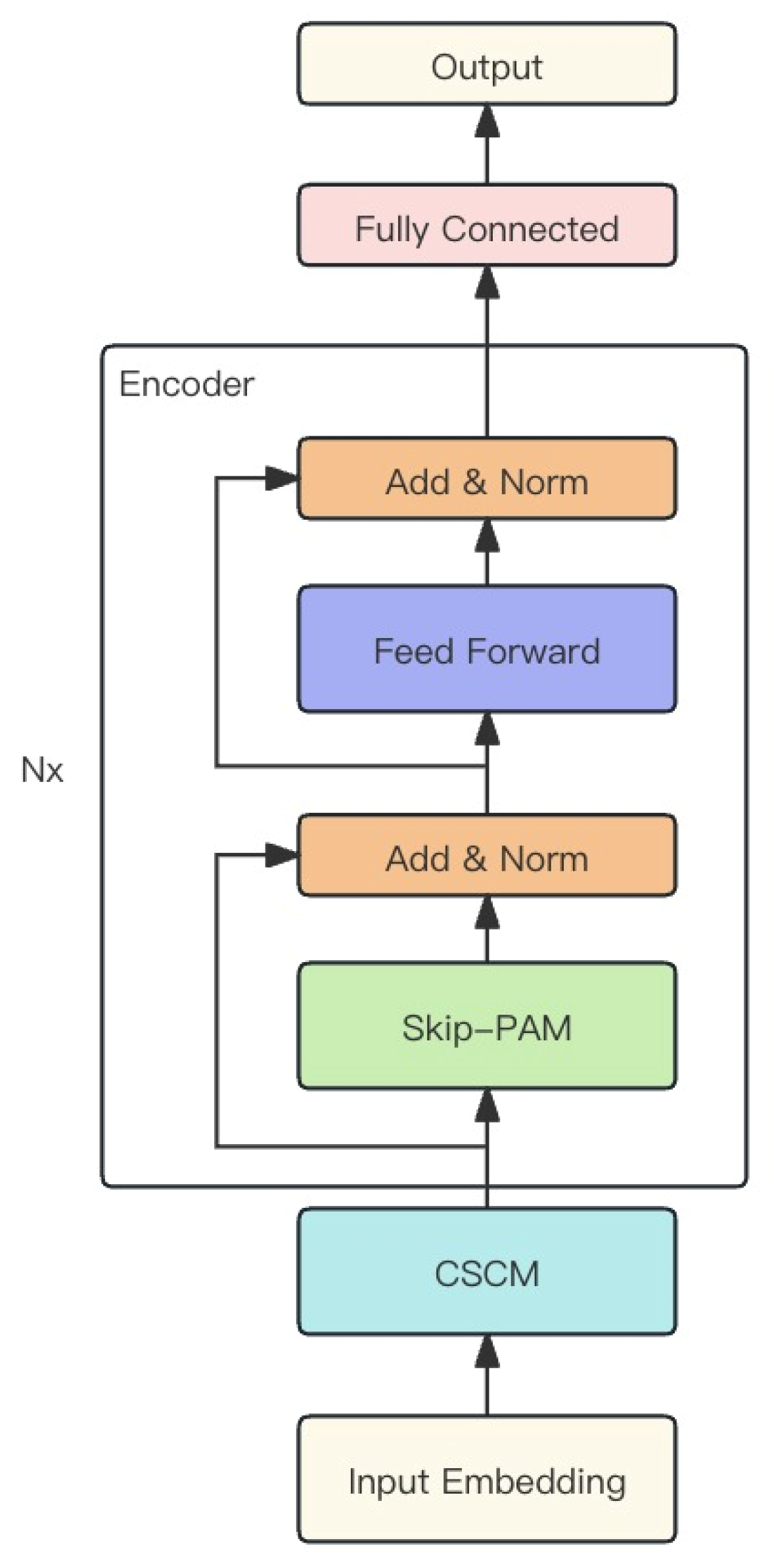
• Introduction of the Skip-PAM aimed at enabling deep learning models to effectively capture long-term and short-term features in long time series. In the encoder, the implementation of a pyramid attention mechanism processes previous feature vectors to obtain long-term dependencies and local features.
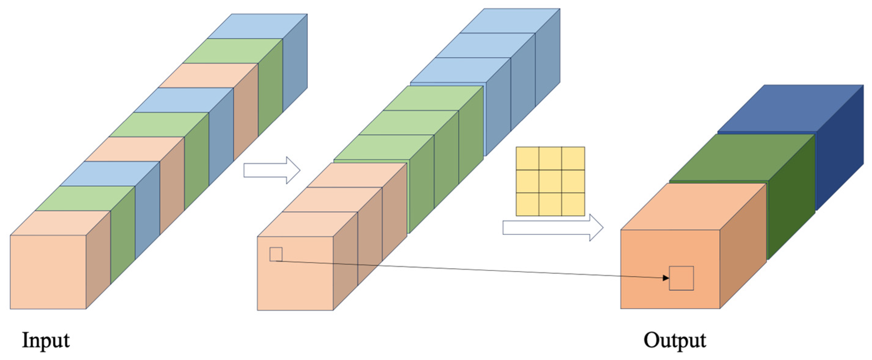
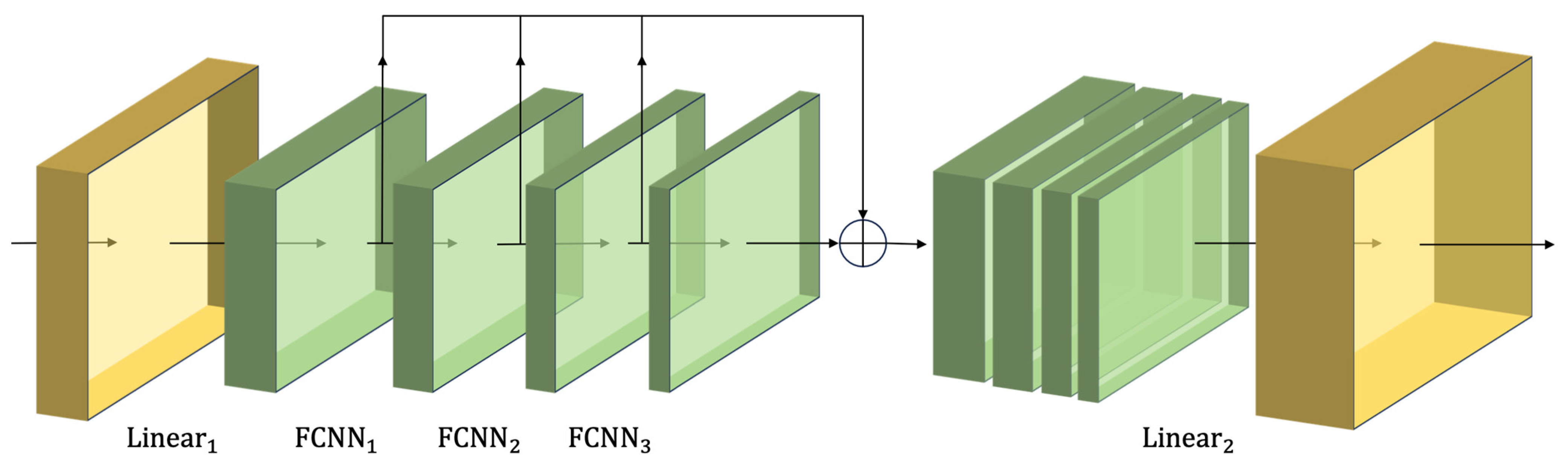
• Improvement of the CSCM aimed at establishing a pyramid data structure for the Skip-PAM. After encoding the input data, coarse-grained feature information across different time step lengths is obtained through the proposed feature convolution.
• Based on three time series datasets, our approach is compared with three baseline methods, achieving a favorable performance.

2. Recent Work

2.1. Time Series Prediction Based on CNN and LSTM

When dealing with long time series data, challenges often arise due to long-term dependency and the loss of short-term information. For instance, in the case of LSTM handling long sequences, as data propagate backward, information features gradually decay over time. Similarly, when using CNN to process time series data, its inherent convolutional operations primarily focus on local neighborhoods, potentially overlooking crucial information from past time points, especially when such information is vital for current predictions. Researchers have explored various methods to address these challenges [15,16]. Oord [17] introduced a CNN variant known as Causal CNN, specifically designed for processing sequence data (Figure 1b). In Causal CNN, the output is not influenced by future inputs, ensuring that convolution operations use only current and past data points. This design prevents information leakage during the prediction of future values in time series data, maintaining the causal sequence of time. However, due to its sequential processing of one time point at a time, Causal CNN requires more computational steps and has a higher time complexity when handling long sequences, limiting its effectiveness in capturing long-term dependencies [18]. Building upon this, Bai [19] proposed a TCN (temporal convolutional network), using stacked causal convolutions to capture the temporal dependencies of time series data. It employs dilated convolutions to increase the receptive field, covering a longer input history (Figure 1d). TCN’s causal convolutions and dilation structure enable it to predict the entire output sequence in a single forward pass, significantly reducing the time complexity. TCN also incorporates residual structures to address the issue of gradient vanishing during training, enhancing network training efficiency. Chen [20] introduced a two-stage attention mechanism model called TPM, which divides the original time series into short-term and long-term features. Short-term features are extracted using CNN, while long-term features are obtained through a piecewise linear regression method (PLR) [21]. The encoder and decoder extract short-term and long-term features, respectively, and combining multi-scale temporal feature information leads to improved prediction results. Lai [22] proposed LSTNet (long-and short-term time series network), utilizing CNN and RNN to capture the short-term and long-term features of time series. It addresses the scale insensitivity issue of neural network models by incorporating an autoregressive model. For capturing long-term features, an innovative Skip-RNN is introduced, allowing backward propagation with specified step lengths (Figure 1c). Skip-RNN can obtain global feature information with fewer nodes. Woo [23] introduced CoST to separate trends and seasonality in time series data and used contrastive learning to capture features in the time and frequency domains. CoST’s contrastive loss in the time domain aids the model in learning trend features, while the frequency domain’s contrastive loss focuses on seasonal features. This approach extracts features at multiple scales from a single time series, where these features are independent but collectively contribute to the prediction task, leading to a more comprehensive understanding of data and an improved prediction accuracy.

2.2. Transformer-Based Time Series Prediction Approaches

In recent years, a series of innovative Transformer-based models have emerged, leveraging advanced architectures and algorithms to capture intricate temporal dependencies, thereby enhancing prediction accuracy and efficiency. Informer [24] effectively addresses long-term time series by utilizing the ProbSparse self-attention mechanism. It optimizes the computational complexity of traditional Transformer models, allowing them to handle longer sequences without sacrificing performance. Its design addresses a fundamental issue in long sequence prediction: how to capture deep dynamics in time series while maintaining computational efficiency. Autoformer [25] is a model that combines autoregressive statistical models with deep learning techniques. Its autoregressive correlation structure is specifically designed to identify and leverage the periodic features of time series, making it more suitable for time series prediction tasks with distinct periodic and trend features. Reformer [26] focuses on addressing issues with long sequences by reducing the computational complexity of self-attention using hash techniques and minimizing memory consumption through reversible layers. Pyraformer [27] adopts a different strategy, utilizing a pyramid structure to capture multi-scale features in time series, revealing rich hierarchical and complex dynamics in sequence data (Figure 2a). This design meets the demand for a more refined understanding of time resolution, particularly crucial in areas like financial market analysis. FEDformer [28] introduces a novel perspective on analyzing time series by performing self-attention in the frequency domain. It uses Fourier and wavelet transforms to unveil patterns hidden behind periodic and seasonal variations in time series. Through intelligent transformations of the data, FEDformer captures important features in the frequency domain that may not be easily discernible in the time domain.

3. Model

The overall framework of the proposed MSFformer is illustrated in Figure 3. Building upon the Pyraformer architecture, our model enhances the attention mechanism in the encoder by innovatively introducing a pyramid attention mechanism across different time step lengths. To construct multi-scale temporal information, we employ feature convolution to build the CSCM, extracting temporal information at a coarser granularity.

3.1. Skip-PAM

This paper introduces an innovative framework, called the Skip-Pyramidal Attention Module (Skip-PAM), as part of the MSFformer model. The objective is to enhance the capability of deep learning models in handling time series data through a multi-level attention mechanism. The core idea of this mechanism is to process input data at different time step lengths, enabling the model to capture time dependencies at various granularities. At lower levels, the model may focus on short-term, fine-grained patterns. In contrast, at higher levels, it can capture more macroscopic trends and periodicities. Unlike PAM, which focuses on weekly and monthly information, Skip-PAM pays more attention to information such as every Monday or the beginning of each month. This kind of multi-scale processing allows the model to capture diverse time-dependent relationships across different levels.

As shown in Figure 2b, Skip-PAM extracts information from the time series at multiple scales through the attention mechanism constructed by the time feature tree. This process involves both intra-scale connections and inter-scale connections. Intra-scale connections involve performing attention calculations between a node and its adjacent nodes within the same scale layer. Inter-scale connections involve attention calculations between a node and its parent node (each parent node having P children) and C child nodes. Specifically, for a node $n_l^s$, $s\in \left[1,S\right]$ denotes the layer scale from the bottom to the top (S layers in total), and $l\in \left[1,l_s\right]$ represents the l-th node in that layer.

$${\mathbb{A}}_l^s=\left\{n_l^s:\left|j-l\right|\le \frac{A-1}{2},1\le j\le \frac{L}{C^{s-1}}\right\}$$

(1)

$${ℂ}_l^s=\left\{n_j^{s-1}:j=l+iC,i=0,1,2\dots \mathrm{if} s\ge 2 \mathrm{else} \varnothing \right\}$$

(2)

$${\mathbb{P}}_l^s=\left\{n_j^{s+1}:j=l \mathrm{mod} \mathrm{P} \mathrm{if} \mathrm{s}\le S-1 \mathrm{else} \varnothing \right\}$$

(3)

$${\mathbb{N}}_l^s={\mathbb{A}}_l^s\cup {ℂ}_l^s\cup {\mathbb{P}}_l^s$$

(4)

where ${\mathbb{A}}_l^s$ represents the adjacent nodes within the scale, $A$ denotes the number of adjacent nodes within the scale, ${ℂ}_l^s$ signifies the child nodes, ${\mathbb{P}}_l^s$ represents the parent node, and ${\mathbb{N}}_l^s$ is the total number of nodes for which the attention mechanism should be computed. So, for the node $n_l^s$, attention can be represented as follows:

$${\stackrel{`}{x}}_i={\displaystyle \sum }_{l\in {\mathbb{N}}_l^s}\frac{\exp \left(\frac{q_i{k}_l^T}{\sqrt{d_x}}\right)v_l}{{{\displaystyle \sum }}_{l\in {\mathbb{N}}_l^s}\exp \left(\frac{q_i{k}_l^T}{\sqrt{d_x}}\right)}$$

(5)

where $q_i$ is the query matrix corresponding to $x_i$; $k_l$ and $v_l$ are the key and value matrices, respectively; $d_x$ is the sequence length; and ${\stackrel{`}{x}}_i$ is the output result through attention.

Through this pyramid attention mechanism, combined with the multi-scale feature convolution mentioned later, a powerful feature extraction network is formed. It can adapt to dynamic changes across various time scales, whether they are short-term oscillations or long-term evolutions.

3.2. Coarser-Scale Construction Module

To adapt to cross-stride feature extraction, we designed a FCNN (feature convolutional layer), as shown in Figure 4. Specifically, it first extracts feature vectors through the desired cross-stride step, concatenates them together, and then performs convolutional operations using a convolutional kernel with a size of $\lceil l/step\rceil$ and a stride of $\lceil l/step\rceil$. The formula is as follows:

$$Output=\mathrm{FCNN}\left(Input\right)$$

(6)

In order to better apply the aforementioned Skip-PAM structure, we constructed a feature tree and designed a CSCM. As shown in Figure 5, we first passed the input sequence through a linear layer to expand the feature dimension to a fixed dimension. Then, we gradually obtained feature information at different scales through feature convolutional layers and concatenated them to form a pyramid-shaped feature structure. Finally, we used a linear layer to restore the feature dimension.

$$M_0={\mathrm{Linear}}_1\left(X\right)$$

(7)

$$M_1={\mathrm{FCNN}}_1\left(M_0\right)$$

(8)

$$M_2={\mathrm{FCNN}}_2\left(M_1\right)$$

(9)

$$M_3={\mathrm{FCNN}}_3\left(M_2\right)$$

(10)

$$M_{CSCM}={\mathrm{Linear}}_2\left(\left[M_0;M_1;M_2;M_3\right]\right)$$

(11)

where $X$ is the input to the CSCM, $Linear$ represents the linear layer, $\mathrm{FCNN}$ is the feature convolution module mentioned in Equation (6), $M_1, M_2,$ and $M_3$ are the consecutive results of feature convolution, $M_{CSCM}$ is the output of the CSCM, and the ‘;’ operation is used to concatenate $M_0, M_1, M_2,$ and $M_3$ along the time dimension.

By passing our data through such a CSCM, we obtained time feature information at different granularities. By stacking the feature convolutional layers, we built a pyramid-shaped feature tree. This not only enabled us to understand the data at multiple levels but also provided a solid foundation for the implementation of the Skip-PAM.

4. Experiment

4.1. Experimental Data

This paper validates the model using three time series datasets with different levels of stationarity, as detailed below:

• ETTh1: The ETT dataset [24] comprises temperature records collected from transformers and six indicators related to voltage load in the period from July 2016 to July 2018. The ETTh1 data, with their hourly collection frequency, are ideal for evaluating the model’s capability to capture cyclical daily patterns and longer-term seasonal trends in energy usage related to environmental temperature fluctuations.
• ETTm1: As a more granular subset of the ETT dataset, ETTm1 provides data at 15 min intervals. This higher-resolution dataset challenges the model to discern subtler short-term variations and abrupt changes in electrical load, which are critical for operational decisions in energy distribution and for responding to rapid demand shifts.
• Electricity [29]: This dataset records the hourly electricity consumption from 2012 to 2014 for 321 customers. It serves as a rich source for examining consumer behavior over multiple years, including variations in consumption due to individual lifestyle patterns, societal events, and differing business operations.

As outlined in

Table 1. Dataset. presents the feature counts, sampling frequencies, data point numbers, as well as the mean, standard deviation, minimum, and maximum for the three datasets.

Dataset	Feature Counts	Sampling Frequencies	Data Point Numbers	Mean	Std	Min	Max
ETTh1	7	1 h	121,940	4.58	25.59	−25.09	46.01
ETTm1	7	15 min	487,760	4.59	25.62	−26.37	46.01
Electricity	321	1 h	7,506,264	2551.88	231,879,417.19	0.00	764,500.00

, all three datasets are partitioned into training, validation, and test sets with a ratio of 6:2:2. Moreover, the data within these three datasets are all in a floating-point format.

4.2. Evaluation Metrics

In this study, we employed three widely used performance evaluation metrics to assess the predictive accuracy of the model: mean square error (MSE), mean absolute error (MAE), and mean absolute percentage error (MAPE). Lower values of these three metrics indicate a superior predictive performance of the model [30].

MSE: The MSE measures the average of the squared differences between the predicted values ${y^{\prime }}_i$ and the actual values $y_i$. This metric gives higher penalties to larger errors, emphasizing the evaluation of larger prediction discrepancies [31]. The formula is expressed as follows:

$$\mathrm{MSE}=\frac{1}{n}{\displaystyle \sum }_{\mathrm{i}=1}^n{\left(y_i-{y^{\prime }}_i\right)}^2$$

(12)

MAE: Similar to the MSE, this metric calculates the average absolute differences between the predicted values ${y^{\prime }}_i$ and the actual observed values $y_i$. It reflects the average magnitude of the deviations of the predicted values from the true values [32]. The formula is expressed as follows:

$$\mathrm{MAE}=\frac{1}{n}{\displaystyle \sum }_{\mathrm{i}=1}^n\left|y_i-{y^{\prime }}_i\right|$$

(13)

MAPE: The MAPE is a measure that calculates the average of the percentage differences between the predicted values ${y^{\prime }}_i$ and the actual values $y_i$. It provides insight into the accuracy of predictions in terms of their deviation from the actual values as a percentage, which can be particularly useful when comparing the performance of forecasting models across different scales of data. The formula is expressed as follows:

$$\mathrm{MAPE}=\frac{1}{n}{\displaystyle \sum }_{\mathrm{i}=1}^n\left|\frac{y_i-{y^{\prime }}_i}{y_i}\right|\times 100\%$$

(14)

4.3. Parameter Settings and Experiment Details

During the experimental process in this chapter, four different prediction time point lengths were set for the datasets: 96, 192, 336, and 720. For the ETTh1 and Electricity datasets, these horizons correspond to future predictions of 4 days, 8 days, 2 weeks, and 1 month, respectively. For the ETTm1 dataset, they represent predictions for 1 day, 2 days, 3.5 days, and 7.5 days into the future, respectively. The prediction task aims at multi-feature forecasting. The encoder layers were set to four, and the attention heads were set to six. Using a time series with a length of 96 as the input, a stride length window of {4, 4, 6} was applied to construct the features, resulting in a tree structure with layers {96, 24, 6, 1}. In the construction process of the Skip-PAM, the inter-scale connecting node, i.e., the inner size, was set to five. In the data preprocessing step, we applied different normalization techniques tailored to the characteristics of each dataset. Specifically, for the ETT dataset, we employed the Z-score normalization method, which transforms the data using the formula $normalized=\left(original-mean\right)/std$. For the Electricity dataset, on the other hand, we utilized a mean-adjusted proportional scaling method, processing the data with the formula $normalized=original/\left(mean+1\right)$.

We adopted Adam as our optimization algorithm, with an initial learning rate of ${10}^{-4}$, which was decreased to one-tenth of its value at the end of each epoch. We set the number of epochs to five. In the experiments of this paper, all the model algorithms were implemented based on the PyTorch and were trained and tested using a single NVIDIA GeForce RTX 4090 GPU.

4.4. Comparative Experiments

To validate the effectiveness of the proposed MSFformer model in this chapter, we conducted training and compared the results with three baseline models. From

Table 2. Comparative experiments. This table describes the experimental results obtained by training the MSFformer and three baseline methods on the ETTh1, ETTm1, and Electricity datasets. The comparison includes results for different prediction lengths (96, 192, 336, 720), with bold formatting indicating a superior performance. The MAPE is presented as a percentage value, and the input time series length during training was consistently set to 96.

Model		Transformer [13]			Informer [24]			Pyraformer [27]			MSFformer (Ours)
Metric		MSE	MAE	MAPE	MSE	MAE	MAPE	MSE	MAE	MAPE	MSE	MAE	MAPE
ETTh1	96	0.9306	0.7750	9.2998	0.9749	0.7814	7.9607	0.7671	0.6515	9.1344	0.6598	0.5774	8.3353
	192	1.0529	0.8226	8.7659	1.0265	0.7917	10.8025	0.8567	0.7038	8.7809	0.6861	0.6009	8.3445
	336	1.1429	0.8757	11.4834	1.0334	0.7751	14.3382	0.9408	0.7564	12.9577	0.8359	0.6898	12.2144
	720	1.0951	0.8278	18.3381	1.2032	0.8694	18.3253	1.0680	0.8346	23.7789	0.9312	0.7424	24.5435
ETTm1	96	0.6548	0.5905	3.0617	0.6374	0.5635	2.5444	0.5293	0.5002	2.4246	0.4926	0.4831	2.3761
	192	0.8633	0.7138	3.7736	0.7303	0.6198	2.5095	0.5432	0.5167	2.2955	0.4955	0.4923	2.3117
	336	1.0364	0.7898	3.8568	1.1851	0.8039	3.5393	0.6930	0.6307	3.3065	0.7266	0.6175	3.1333
	720	1.1136	0.8301	3.9590	1.2199	0.8373	3.5921	0.9290	0.7305	3.6573	0.7825	0.6410	3.2721
Electricity	96	0.3326	0.3971	4.0659	0.4854	0.4917	5.4207	0.4965	0.2939	1.7223	0.4698	0.2636	1.4362
	192	0.3434	0.4083	4.6065	0.5001	0.5102	5.7366	0.5854	0.3061	1.9153	0.7943	0.2619	1.6628
	336	0.3631	0.4271	5.1759	0.4352	0.4734	5.3652	1.4643	0.3134	2.3761	1.4602	0.2843	2.1562
	720	0.3832	0.4244	5.2572	0.5197	0.5311	5.7170	4.0697	0.3762	3.1227	4.1038	0.3290	2.5450

, it can be concluded that, across all the datasets, especially in the case of the ETTh1 and ETTm1 datasets, the MSFformer model demonstrates the best overall performance, followed by Pyraformer. This suggests that MSFformer is particularly effective in long time series prediction tasks, leveraging information from multiple scales. The Skip-PAM allows the model to combine both long-term and short-term features, enhancing its predictive capabilities. For the ETTh1 dataset, MSFformer outperforms all the other comparison methods in terms of the MSE and MAE metrics but performs poorly on the MAPE metric. The higher values of the MAPE, despite the MSE imposing heavier penalties on larger errors, may be attributed to the asymmetry of the MAPE—it penalizes negative errors (when the predicted value exceeds the actual value) more than positive errors. On the ETTm1 dataset, MSFformer significantly surpasses the Transformer and Informer models across all the evaluation metrics and is also slightly better than Pyraformer in most cases. This underscores the superior capability of MSFformer in capturing subtle changes within short intervals, especially at shorter prediction lengths such as 96 and 192. For the Electricity dataset, MSFformer exhibits suboptimal performance in the MSE metric, while achieving the best performance in the MAE and MAPE among all the model methods. This discrepancy might be attributed to larger prediction errors at certain time points, where the MSE amplifies such errors, whereas the MAE and MAPE indicate that the MSFformer model still excels in time series prediction tasks. Overall, the MSFformer model outperforms the three baseline methods. In terms of the MAE, it achieves a maximum improvement of 26.95%, 31.03%, and 35.87% over the Transformer model in the three datasets. Additionally, for the ETTh1 and ETTm1 datasets, the MSFformer model achieves a maximum improvement of 34.84% and 42.60%, respectively, in the MSE metric.

The visual analysis presented in Figure 6 unambiguously substantiates the pronounced superiority of our proposed MSFformer model in terms of precision and the dynamic capturing of time series data. Employing a multi-scale feature extraction strategy, the model demonstrates exemplary performance across diverse forecasting horizons, a fact which becomes evident when juxtaposed with the Pyraformer model’s comparative analysis. Particularly with regard to the identification and prediction of peak phenomena in time series, MSFformer manifests a heightened sensitivity and a superior predictive prowess, attributable to its intricate mechanism for discerning both long- and short-term dependencies. Even as the forecasting window extends, posing increased predictive challenges, the MSFformer maintains laudable accuracy. Furthermore, an augmentation in input length bolsters the model’s performance, highlighting the efficacy of multi-scale feature extraction in harvesting extensive historical insights and pinpointing pivotal temporal dependencies. These findings not only emphasize the robustness of the MSFformer in navigating the complexities of time series prediction but also its adaptability across varying data scales, enhancing its potential for wide-ranging applications in complex forecasting scenarios.

To demonstrate that our approach can integrate information across multiple temporal scales, we utilized a synthetic hourly dataset [27], with multi-range dependencies, for our experiments. This dataset was synthesized by linearly combining three sine functions with different periods: 24, 168, and 720 h, representing daily (short-term), weekly (mid-term), and monthly (long-term) temporal dependencies, respectively. In the experimental setup, both the input length and the prediction length were set to 720, with all the basic settings remaining consistent with previous comparative experiments except for the window size and inner size. Given that the synthetic time series exhibited long-range correlations in both their deterministic and stochastic components, it was crucial for the model to effectively capture such dependencies to accurately forecast the subsequent 720 data points. The experimental results are summarized in

Table 3. Experiments results on the synthetic dataset. The table describes the MSE and MAE values of different methods on the synthetic dataset, with the best results highlighted in bold and the second-best results underlined.

Model	MSE	MAE
Transformer	3.550	1.477
Informer	7.546	2.092
Pyraformer	1.176	0.849
${\mathrm{MSFformer}}_{24,6,5}$	1.103	0.818
${\mathrm{MSFformer}}_{20,6,6}$	1.054	0.802

, where ${\mathrm{MSFformer}}_{24,6,5}$ has a window size of {24, 6, 5}, corresponding to a tree structure of {720, 30, 5, 1} and an inner size of 7, and ${\mathrm{MSFformer}}_{20,6,6}$ has a window size of {20, 6, 6}, corresponding to a tree structure of {720, 36, 6, 1}, and an inner size of 13. Both configurations of our MSFformer variant achieved the best results among all the methods, with ${\mathrm{MSFformer}}_{20,6,6}$ showing a 10.37% improvement over the best Pyraformer method in the MSE and an 5.54% improvement in the MAE. Figure 7 visualizes the forecasting results of ${\mathrm{MSFformer}}_{20,6,6}$. Therefore, in long-term time series forecasting tasks, our approach, which integrates features of multiple granularities and captures characteristics across time steps, is indeed capable of effectively capturing multi-scale information.

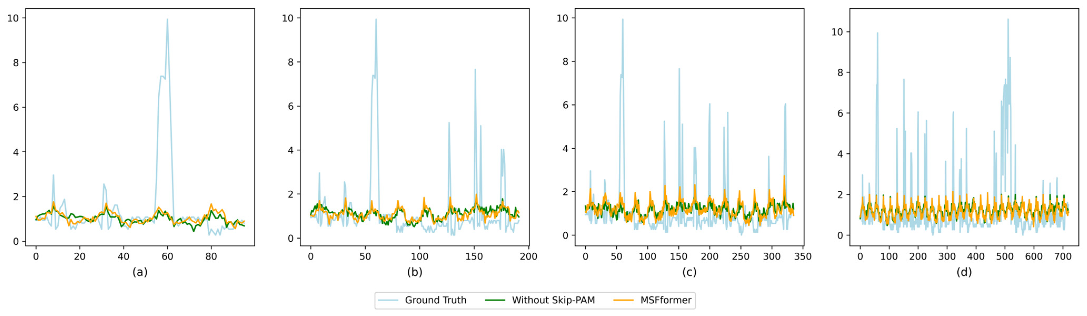
4.5. Ablation Experiments

In the MSFformer model, the key components are Skip-PAM and CSCM. Since CSCM serves Skip-PAM, it is not feasible to remove the CSCM while retaining the Skip-PAM. Therefore, in our ablation experiments, we compared the original model with a model where the Skip-PAM had been removed.

From

Table 4. MSFformer Ablation Experiments. This table describes the results of the ablation experiments conducted on the MSFformer model for three datasets. The MSE and MAE are used as the evaluation metrics, with bold formatting indicating lower values, which are desirable.

Model		MSFformer		Without Skip-PAM
Metric		MSE	MAE	MSE	MAE
ETTh1	96	0.6598	0.5774	0.7530	0.6487
	192	0.6861	0.6009	0.8308	0.6957
	336	0.8359	0.6898	0.9078	0.7418
	720	0.9312	0.7424	1.0365	0.8223
ETTm1	96	0.4926	0.4831	0.5541	0.5082
	192	0.4955	0.4923	0.5365	0.5071
	336	0.7266	0.6175	0.7585	0.6262
	720	0.7825	0.6410	0.8831	0.7326
Electricity	96	0.4698	0.2636	0.4816	0.2791
	192	0.7943	0.2619	0.8023	0.2667
	336	1.4602	0.2843	1.4744	0.3011
	720	4.1038	0.3290	4.1433	0.3576

, it can be concluded that the models without the Skip-PAM exhibit a poorer performance across all three datasets. This suggests that the pyramid feature model we constructed effectively connects the required feature information, disregarding nodes with a low correlation. This not only enhances the accuracy of the model but also, to some extent, reduces the computational complexity, accelerating the training iterations of the model. In the ablation experiments, it is observed that the MSFformer, compared to the model without the Skip-PAM, achieves an average improvement of 10.34%, 5.44%, and 5.24% in MAE across the three datasets. Additionally, in terms of the MSE, there is an average improvement of 11.97%, 8.58%, and 1.34%. This indicates that the Skip-PAM component involved in MSFformer performs better on stationary time series, more accurately capturing the embedded temporal features.

Figure 8 shows the results of the Electricity dataset at different prediction lengths under the same input conditions. The introduction of the Skip-PAM significantly enhances the model’s capability to capture long-term trends. By integrating multi-scale temporal information, the Skip-PAM enables the model to grasp long-term features more accurately, as evidenced by the closer alignment between the trend tracking of the MSFformer with Skip-PAM and the actual values. Moreover, the addition of the Skip-PAM not only improves the model’s ability to capture long-term trends but also enhances its precision in detecting local features, particularly in identifying peak values. This is vividly demonstrated in all sub-figures of Figure 8, especially the peaks near position 59 (a) and at positions 150 (b), 325 (c), and 600 (d), highlighting our method’s efficacy in preserving fine-grained features while extracting large-scale characteristics. In conclusion, the ablation study vividly illustrates the critical importance of the Skip-PAM component for the MSFformer model. It not only substantially improves the model’s proficiency in forecasting long-term trends and accurately detecting local features but also demonstrates the efficiency and accuracy of our approach in tackling time series forecasting tasks. This outcome emphasizes the significance of incorporating multi-scale feature integration when designing time series prediction models.

4.6. Hyperparameter Study

To explore the impact of key parameters in Skip-PAM and crucial encoder parameters on the overall performance of the model, we will hereby conduct a study on the stride window parameters, inner size parameters, as well as the number of attention heads and encoder layers.

(1)

Study on Stride Window Size Parameter

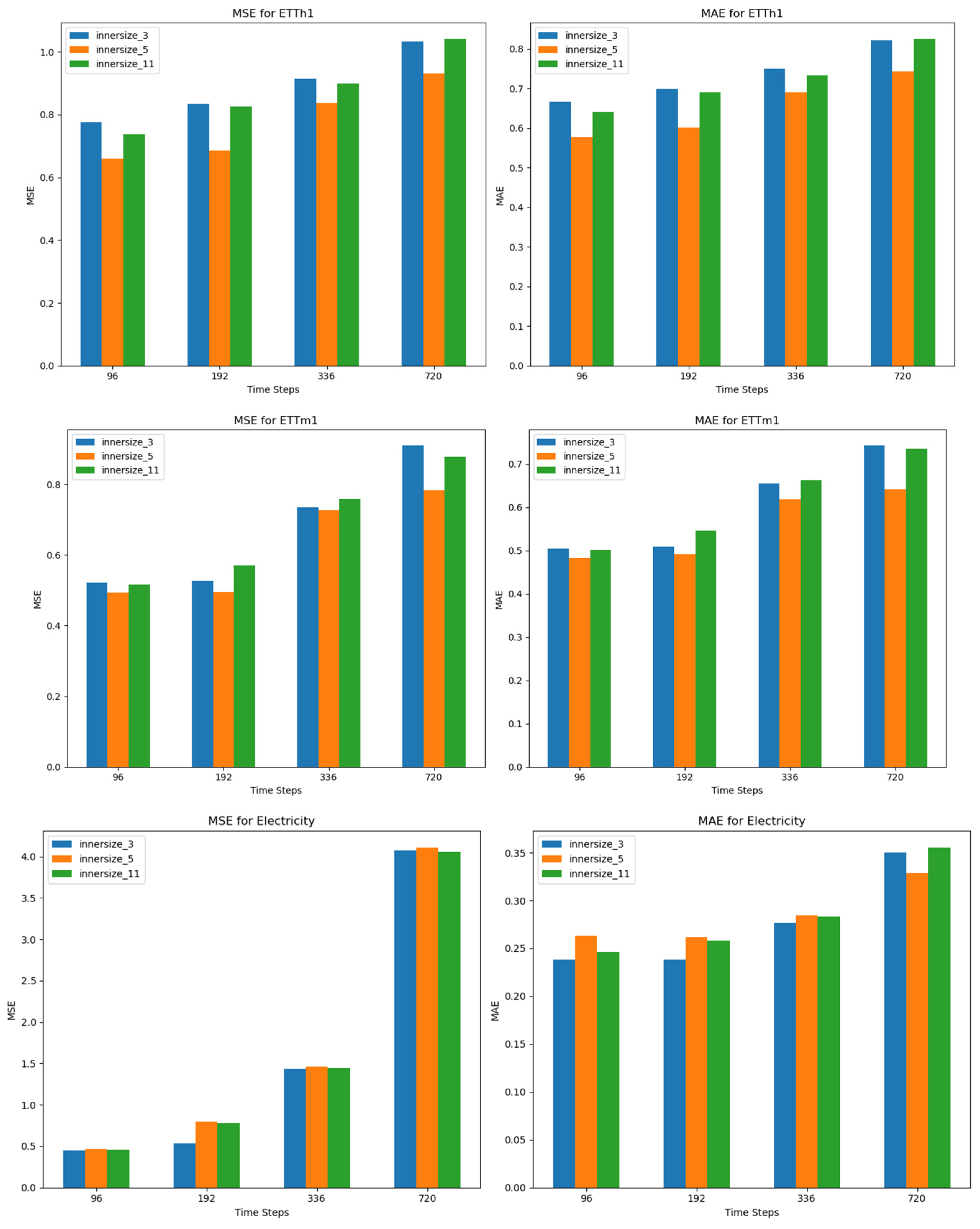
The most crucial parameter in Skip-PAM and CSCM is the stride window size, determining the scale and dimension of the feature tree we construct and influencing the degree of correlation between nodes. In the previous experiments, we utilized a stride window of {4, 4, 6}, resulting in a feature tree structure of {96, 24, 6, 1} when using an input length of 96. Additionally, for an input length of 96, we designed two other window sizes: {3, 6, 6} and {3, 4, 8}, forming tree structures of {96, 32, 6, 1} and {96, 32, 8, 1}, respectively.

From

Table 5. Stride window size parameter study. This table describes the performance of the MSFformer on three datasets using different sizes of stride window time intervals. The time stride configurations are {4, 4, 6}, {3, 6, 6}, and {3, 4, 8}. The evaluation metrics are the MSE and the MAE, with bold formatting indicating the best performance in these two metrics.

Window Size		{4, 4, 6}		{3, 6, 6}		{3, 4, 8}
Metric		MSE	MAE	MSE	MAE	MSE	MAE
ETTh1	96	0.6598	0.5774	0.7577	0.6531	0.7696	0.6595
	192	0.6861	0.6009	0.8374	0.6982	0.8262	0.6923
	336	0.8359	0.6898	0.9116	0.7431	0.9023	0.7401
	720	0.9312	0.7424	1.0564	0.8337	1.0450	0.8190
ETTm1	96	0.4926	0.4831	0.5125	0.4993	0.5048	0.4933
	192	0.4955	0.4923	0.5893	0.5589	0.5592	0.5474
	336	0.7266	0.6175	0.6934	0.6302	0.7043	0.6334
	720	0.7825	0.6410	0.9332	0.7443	0.8564	0.7175
Electricity	96	0.4698	0.2636	0.4509	0.2401	0.4443	0.2311
	192	0.7943	0.2619	0.7830	0.2568	0.7783	0.2483
	336	1.4602	0.2843	1.4362	0.2740	1.4341	0.2713
	720	4.1038	0.3290	4.0574	0.3261	4.0695	0.3472

, it can be summarized that, for the ETTh1 and ETTm1 datasets, the configuration of {4, 4, 6} performs the best among the three designed stride window configurations. This configuration may offer a more balanced pyramid shape, providing a stable reference framework for time series prediction. This implies that the model can more effectively capture key patterns in the time series, being less susceptible to random fluctuations. Therefore, in terms of average performance and error rates, this stride configuration is superior compared to the others. For the Electricity dataset, the stride configuration of {3, 4, 8} performs the best. This could be related to the characteristics of the dataset, as electricity usage data typically involve a broader time range and more complex temporal dependencies. In electricity usage scenarios, not only recent usage is important, but also correlations with more distant past time points need consideration. Thus, larger stride lengths can better capture these long-term temporal dependencies, thereby improving the model’s accuracy in predicting electricity usage trends.

(2)

Inner Size Parameter Study

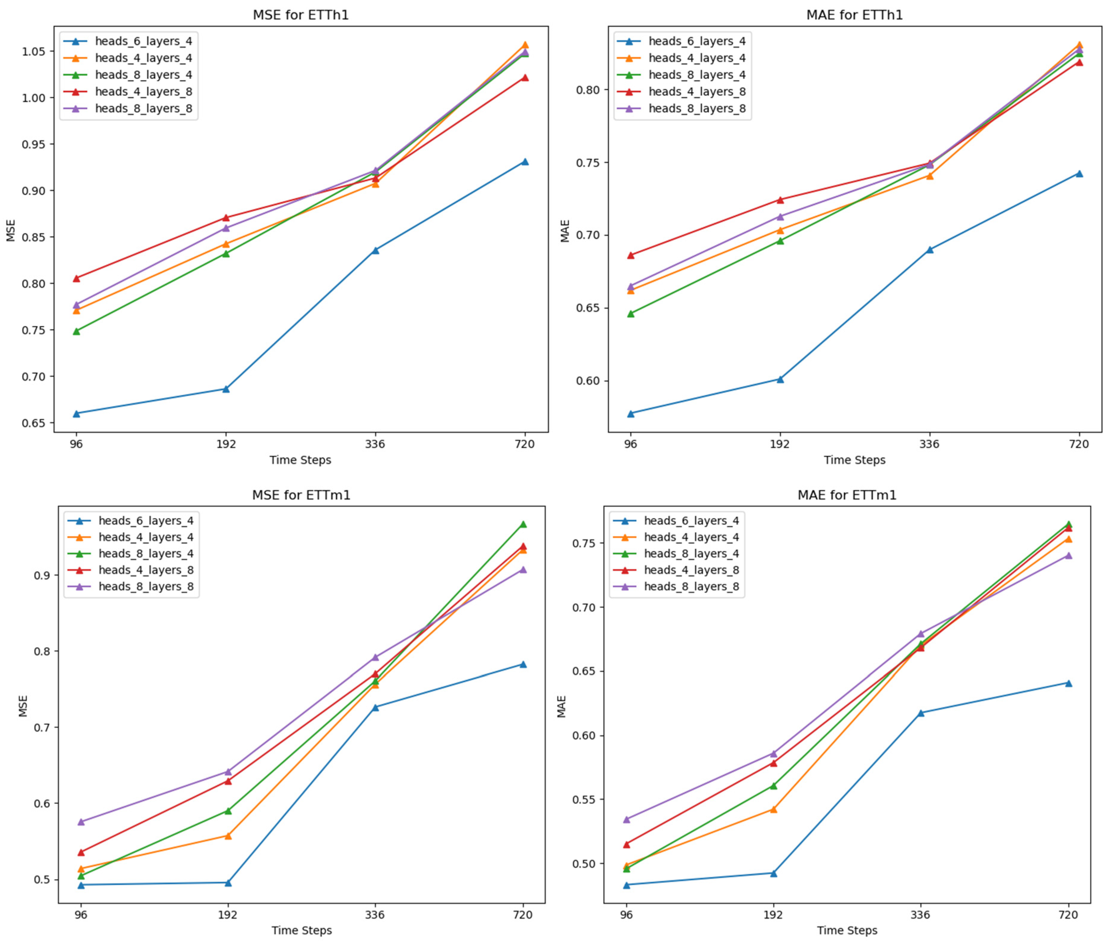
Within the Skip-PAM, another crucial parameter determining the attention structure is the inner size parameter. This parameter signifies how many neighboring nodes a particular node should connect with within a given scale. In the previous experiments, the inner size parameter was set to five. To investigate the impact of this parameter, experiments were also conducted with inner size parameters set to 3 and 11.

From Figure 9, it can be summarized that, for the datasets ETTh1 and ETTm1, setting the inner size to five produces the best results. This might be attributed to the fact that setting the inner size to three, during which the model captures a very short time range, makes it insufficient for capturing long-term dependencies and patterns in the time series. On the other hand, setting the inner size to 11 may introduce too much non-critical information, leading to redundancy or less relevant information in the data processed by the model. In contrast, setting the inner size to five provides a balance, capturing sufficient time information to identify critical patterns while avoiding excessive interference from irrelevant information. For the Electricity dataset, setting the inner size to three yields the best results. This might be closely related to the characteristics of electricity usage data, where usage is often more closely related to adjacent time periods. Therefore, setting the inner size to 5 and 11 may introduce historical information less relevant to the immediate electricity usage trend, thereby reducing prediction accuracy.

(3)

Study on Attention Heads and Encoder Layers Parameters

The proposed model in this study is fundamentally an improvement based on the Transformer model. Therefore, the number of attention heads and encoder layers is crucial for the performance of the MSFformer model. In the previous experiments, the number of attention heads and encoder layers were set to six and four, respectively. To investigate the impact of these two parameters, experiments were conducted, with the number of attention heads being {4, 6, 8} and the encoder layers being {4, 6, 8}.

From Figure 10, it can be concluded that, for the datasets ETTh1 and ETTm1, the model performs best when the number of attention heads is six and the number of encoder layers is four. In this configuration, the model can better capture complex relationships and features in the data. Increasing the number of encoder layers can lead to overfitting on the dataset, resulting in a poorer overall performance. For the Electricity dataset, the model performs best when the number of attention heads is eight and the number of encoder layers is four. This may be due to the larger feature dimensions of the dataset. By increasing the number of attention heads, the model has a larger parameter capacity, allowing it to more fully capture complex relationships and features in the data.

5. Conclusions

In this paper, a multi-scale feature extraction model, MSFformer, based on Transformer models, was proposed to address the issue of the insufficient extraction of long-term dependencies and short-term features in long time series prediction tasks. Specifically, a novel feature convolution method was introduced in the CSCM to obtain coarse-grained information, building a pyramid-shaped data structure through convolution operations with specified strides, extracting time feature information continuously. The Skip-PAM, a cross-stride attention mechanism, was then constructed on this basis, extracting the relevance of adjacent nodes, parent nodes, and child nodes with a specified stride to build an attention mechanism. MSFformer demonstrated superior performance, on average, on three datasets compared to three baseline methods, indicating the effectiveness of our model. Additionally, ablation experiments conducted on the MSFformer model highlighted the significant contribution of the proposed key modules toward performance improvement. Lastly, a study on important hyperparameters revealed different optimal parameters for different datasets.

The limitations of this study include the use of designed feature convolution for constructing coarse-grained data in the MSFformer, which may not efficiently extract features. Exploring efficient methods for constructing coarse-grained data is an area for further research. Additionally, the three layers constructed in the experiments may not be optimal for longer prediction horizons. Further investigation into the relationship between the number of layers and model performance for longer prediction horizons is warranted. Moreover, the temporal granularity of the datasets used in this paper is daily and hourly, and future research could explore the model’s performance on datasets with different levels of granularity and from various domains. For the Electricity dataset, the significant MSE loss indicates that our model’s capability to predict larger errors remains limited. In future work, we will delve deeper into enhancing our model’s predictive accuracy for substantial deviations. In the presentation of our results, we did not detail how the features extracted from the historical sequences influenced the predictions. In our future work, we plan to enhance the interpretability of our model by further exploring and elucidating the specific impact of these features.

References

1. Bao, W.; Yue, J.; Rao, Y. A deep learning framework for financial time series using stacked autoencoders and long-short term memory. PLoS ONE 2017, 12, e0180944. [Google Scholar] [CrossRef] [PubMed]
2. Chase, C.W. Demand-Driven Forecasting: A Structured Approach to Forecasting; John Wiley & Sons: Hoboken, NJ, USA, 2013. [Google Scholar]
3. McGovern, A.; Elmore, K.L.; Gagne, D.J.; Haupt, S.E.; Karstens, C.D.; Lagerquist, R.; Smith, T.; Williams, J.K. Using artificial intelligence to improve real-time decision-making for high-impact weather. Bull. Am. Meteorol. Soc. 2017, 98, 2073–2090. [Google Scholar] [CrossRef]
4. Hyndman, R.J.; Athanasopoulos, G. Forecasting: Principles and Practice; OTexts: Melbourne, Australia, 2018. [Google Scholar]
5. Tran, T.H.; Nguyen, L.M.; Yeo, K.; Nguyen, N.; Phan, D.; Vaculin, R.; Kalagnanam, J. An End-to-End Time Series Model for Simultaneous Imputation and Forecast. arXiv 2023, arXiv:2306.00778. [Google Scholar]
6. Lecun, Y.; Bottou, L.; Bengio, Y.; Haffner, P. Gradient-based learning applied to document recognition. Proc. IEEE 1998, 86, 2278–2324. [Google Scholar] [CrossRef]
7. Zaremba, W.; Sutskever, I.; Vinyals, O. Recurrent neural network regularization. arXiv 2014, arXiv:1409.2329. [Google Scholar]
8. Ismail Fawaz, H.; Forestier, G.; Weber, J.; Idoumghar, L.; Muller, P.A. Deep learning for time series classification: A review. Data Min. Knowl. Discov. 2019, 33, 917–963. [Google Scholar] [CrossRef]
9. Borovykh, A.; Bohte, S.; Oosterlee, C.W. Conditional time series forecasting with convolutional neural networks. arXiv 2017, arXiv:1703.04691. [Google Scholar]
10. Lipton, Z.C.; Kale, D.C.; Elkan, C.; Wetzel, R. Learning to diagnose with LSTM recurrent neural networks. arXiv 2015, arXiv:1511.03677. [Google Scholar]
11. Hochreiter, S.; Schmidhuber, J. Long short-term memory. Neural Comput. 1997, 9, 1735–1780. [Google Scholar] [CrossRef]
12. Graves, A.; Schmidhuber, J. Framewise phoneme classification with bidirectional LSTM and other neural network architectures. Neural Netw. 2005, 18, 602–610. [Google Scholar] [CrossRef]
13. Vaswani, A.; Shazeer, N.; Parmar, N.; Uszkoreit, J.; Jones, L.; Gomez, A.N.; Kaiser, Ł.; Polosukhin, I. Attention is all you need. In Proceedings of the Advances in Neural Information Processing Systems 30, Long Beach, CA, USA, 4–9 December 2017. [Google Scholar]
14. Zeng, A.; Chen, M.; Zhang, L.; Xu, Q. Are transformers effective for time series forecasting? In Proceedings of the AAAI Conference on Artificial Intelligence, Washington, DC, USA, 7–14 February 2023; Volume 37. [Google Scholar]
15. Shih, S.Y.; Sun, F.K.; Lee, H.Y. Temporal pattern attention for multivariate time series forecasting. Mach. Learn. 2019, 108, 1421–1441. [Google Scholar] [CrossRef]
16. Liu, M.; Zeng, A.; Chen, M.; Xu, Z.; Lai, Q.; Ma, L.; Xu, Q. Scinet: Time series modeling and forecasting with sample convolution and interaction. Adv. Neural Inf. Process. Syst. 2022, 35, 5816–5828. [Google Scholar]
17. Van Den Oord, A.; Dieleman, S.; Zen, H.; Simonyan, K.; Vinyals, O.; Graves, A.; Kalchbrenner, N.; Senior, A.; Kavukcuoglu, K. Wavenet: A generative model for raw audio. arXiv 2016, arXiv:1609.03499. [Google Scholar]
18. Budhathoki, K.; Vreeken, J. Origo: Causal inference by compression. Knowl. Inf. Syst. 2018, 56, 285–307. [Google Scholar] [CrossRef]
19. Bai, S.; Kolter, J.Z.; Koltun, V. An empirical evaluation of generic convolutional and recurrent networks for sequence modeling. arXiv 2018, arXiv:1803.01271. [Google Scholar]
20. Chen, Y.; Lin, W.; Wang, J.Z. A dual-attention-based stock price trend prediction model with dual features. IEEE Access 2019, 7, 148047–148058. [Google Scholar] [CrossRef]
21. Wagner, A.K.; Soumerai, S.B.; Zhang, F.; Ross-Degnan, D. Segmented regression analysis of interrupted time series studies in medication use research. J. Clin. Pharm. Ther. 2002, 27, 299–309. [Google Scholar] [CrossRef]
22. Lai, G.; Chang, W.C.; Yang, Y.; Liu, H. Modeling long-and short-term temporal patterns with deep neural networks. In Proceedings of the 41st International ACM SIGIR Conference on Research & Development in Information Retrieval, Ann Arbor, MI, USA, 8–12 July 2018. [Google Scholar]
23. Woo, G.; Liu, C.; Sahoo, D.; Kumar, A.; Hoi, S. CoST: Contrastive learning of disentangled seasonal-trend representations for time series forecasting. arXiv 2022, arXiv:2202.01575. [Google Scholar]
24. Zhou, H.; Zhang, S.; Peng, J.; Zhang, S.; Li, J.; Xiong, H.; Zhang, W. Informer: Beyond efficient transformer for long sequence time-series forecasting. In Proceedings of the AAAI Conference on Artificial Intelligence, Virtually, 2–9 February 2021; Volume 35. [Google Scholar]
25. Wu, H.; Xu, J.; Wang, J.; Long, M. Autoformer: Decomposition transformers with auto-correlation for long-term series forecasting. Adv. Neural Inf. Process. Syst. 2021, 34, 22419–22430. [Google Scholar]
26. Kitaev, N.; Kaiser, Ł.; Levskaya, A. Reformer: The efficient transformer. arXiv 2020, arXiv:2001.04451. [Google Scholar]
27. Liu, S.; Yu, H.; Liao, C.; Li, J.; Lin, W.; Liu, A.X.; Dustdar, S. Pyraformer: Low-complexity pyramidal attention for long-range time series modeling and forecasting. In Proceedings of the International Conference on Learning Representations, Virtually, 3–7 May 2021. [Google Scholar]
28. Zhou, T.; Ma, Z.; Wen, Q.; Wang, X.; Sun, L.; Jin, R. Fedformer: Frequency enhanced decomposed transformer for long-term series forecasting. In Proceedings of the International Conference on Machine Learning, PMLR, Baltimore, MD, USA, 17–23 July 2022. [Google Scholar]
29. Electricity Load Diagrams 2011–2014. Available online: https://archive.ics.uci.edu/ml/datasets/ElectricityLoadDiagrams20112014 (accessed on 1 November 2023).
30. Willmott, C.J.; Matsuura, K. Advantages of the mean absolute error (MAE) over the root mean square error (RMSE) in assessing average model performance. Clim. Res. 2005, 30, 79–82. [Google Scholar] [CrossRef]
31. Chai, T.; Draxler, R.R. Root mean square error (RMSE) or mean absolute error (MAE)?–Arguments against avoiding RMSE in the literature. Geosci. Model Dev. 2014, 7, 1247–1250. [Google Scholar] [CrossRef]
32. Hyndman, R.J.; Koehler, A.B. Another look at measures of forecast accuracy. Int. J. Forecast. 2006, 22, 679–688. [Google Scholar] [CrossRef]
Figure 1. Existing sequence modeling architectures for time series forecasting.
Mathematics 12 00973 g001
Figure 2. PAM and Skip-PAM. The point of divergence lies in the node connection method.
Mathematics 12 00973 g002
Figure 3. MSFformer. The input data are encoded and fed into the CSCM, constructing a pyramid-shaped data structure. They then enter the encoder layer with Skip-PAM and are ultimately output through a fully connected layer.
Mathematics 12 00973 g003
Figure 4. Feature convolution layer. The far left shows the original input time series, which are concatenated together through our specified stride (indicated by the same color) to form the concatenated block, as shown in the middle cube in the image. Then, they each go through convolution operations to produce our output. The checkered rectangle depicted above the arrow on the right represents the convolution kernel.
Mathematics 12 00973 g004
Figure 5. CSCM. The input data are concatenated after being processed by different convolutional kernel sizes. The figure, from left to right, sequentially shows X ,   M 0 ,   M 1 ,   M 2 ,   M 3 , M 0 ; M 1 ; M 2 ; M 3 , and M C S C M . (Here, denotes the concatenation operation, which combines M 0 ,   M 1 ,   M 2 ,   and   M 3 into M 0 ; M 1 ; M 2 ; M 3 .
Mathematics 12 00973 g005
Figure 6. Comparison experiment of the oil temperature feature in the ETTh1 dataset. Each subplot displays the comparison between the actual values, Pyraformer predictions, and MSFformer predictions. The figure consists of a total of sixteen subplots arranged in four rows and four columns, where each row represents a different prediction length of 96, 192, 336, and 720, respectively, and each column corresponds to a different input length of 96, 192, 336, and 720, respectively.
Mathematics 12 00973 g006
Figure 7. Visualization results for the synthetic dataset. The figure presents a comparative experiment between the actual values and the predicted values by the MSFformer model, with both the input and prediction lengths set to 720. The horizontal axis represents the time points, while the vertical axis represents the values.
Mathematics 12 00973 g007
Figure 8. Ablation study on feature MT_121 in the Electricity dataset. Each image shows a comparison among the true values, the MSFformer-predicted values, and the predicted values after ablation, using the MT_121 feature of the Electricity dataset (ad). The input time steps are consistently 96, with the row having prediction lengths of {96, 192, 336, 720}, respectively.
Mathematics 12 00973 g008
Figure 9. Inner size parameter study This figure illustrates the results of the inner size parameter study on different datasets, where the inner size parameter is set to 3, 5, and 11. The input time step length is 96, and the stride window size parameter is {4, 4, 6}.
Mathematics 12 00973 g009
Figure 10. Study on attention heads and encoder layers parameters. This figure illustrates the MSE and MAE values for three datasets under different combinations of attention heads and encoder layers. The combinations considered are {6, 4}, {4, 4}, {8, 4}, {4, 8}, and {8, 8}. Other combinations, where the MSE and MAE values were higher than those mentioned, are not explicitly marked in the figure.
Mathematics 12 00973 g010aMathematics 12 00973 g010b