Research on Deep Q-Network Hybridization with Extended Kalman Filter in Maneuvering Decision of Unmanned Combat Aerial Vehicles

Abstract

To adapt to the development trend of intelligent air combat, it is necessary to research the autonomous generation of maneuvering decisions for unmanned combat aerial vehicles (UCAV). This paper presents a maneuver decision-making method for UCAV based on a hybridization of deep Q-network (DQN) and extended Kalman filtering (EKF). Firstly, a three-dimensional air combat simulation environment is constructed, and a flight motion model of UCAV is designed to meet the requirements of the simulation environment. Secondly, we evaluate the current situation of UCAV based on their state variables in air combat, for further network learning and training to obtain the optimal maneuver strategy. Finally, based on the DQN, the system state equation is constructed using the uncertain parameter values of the current network, and the observation equation of the system is constructed using the parameters of the target network. The optimal parameter estimation value of the DQN is obtained by iteratively updating the solution through EKF. Simulation experiments have shown that this autonomous maneuver decision-making method hybridizing DQN with EKF is effective and reliable, as it can eliminate the opponent and preserve its side.

1. Introduction

With the rapid advances in technologies such as wireless technology, electronic circuits, and aerospace materials, unmanned combat aerial vehicles (UCAVs) are endowed with superior performance, capable of handling complex combat tasks, and performing excellently in military applications [1]. The emergence of UCAVs has reshaped the structure of military weapons, expanding the battlefield from flat space to three-dimensional space. The combat capabilities of UCAVs cover multiple combat missions with different functions of reconnaissance, surveillance, localization, target guidance, and ground attack. UAVs play an irreplaceable role in harsh environments and dangerous mission areas, for which there is a need to study how to combine artificial intelligence and unmanned fighters for application in real combat [2]. In the context of intelligent air combat, the degree of intelligence is the primary manifestation of intelligent air combat. Intelligent air combat involves a wide range of operational elements, and there is an urgent need to correctly analyze and assess the development and changes in the situation under intelligent air combat. It is necessary to fully utilize intelligent information-processing methods to plan global elements, intelligently control the entire period of air combat airspace, constantly grasp the opportunity of airspace initiative, and consolidate air power [3]. The combination of artificial intelligence and unmanned fighter aircraft can not only provide maneuvering suggestions for human-piloted fighter aircraft but also realize the unmanned flight of fighter aircraft [4]. Intelligent air combat requires breakthroughs in algorithms for UCAVs to move toward intelligence and maximize their effectiveness.

At present, a large number of scholars have conducted prior research on the methods of maneuvering decision-making for UCAVs, discussing and proposing solutions through scientific methods under their assumptions. According to the core methods, it can be roughly divided into two categories. One method is based on traditional mathematical solutions, such as the influence diagram method [5], genetic optimization algorithm [6], game theory [7,8], and so on. This type of method has a clear mathematical expression, but it is difficult to solve and is effective only for simple air combat environments. The second is based on data learning methods, such as Monte Carlo search [9], approximate dynamic programming [10], neural network [11], etc. These methods are commonly used in the field of maneuvering decision-making at present. For example, the method in the ADP article is only used for solving two-dimensional aircraft, and the maneuver instructions only include left turn, right turn, and hold.

However, aerial combat, with airborne artillery and air-to-air missiles as the main attack weapons, combined with the air battlefield situation and maneuver decision-making, is a highly complex, real-time, and high-risk game confrontation process [12]. Intelligent algorithms represented by deep learning and reinforcement learning have shown significant advantages in air combat, due to their strong perception ability and outstanding decision-making ability [13,14]. In particular, the use of DQN has achieved great success in Atari games in the past, providing a solution to the maneuvering decision-making problem of unmanned fighter jets. However, because the parameters of the DQN are updated through a random gradient descent method, the parameters are easily affected by the experience pool and target network, resulting in a significant deviation between the estimated and true values of the model parameters. This parameter uncertainty can affect the stability and convergence of DQN training results, resulting in poor reliability of maneuvering decisions for UCAVs.

Therefore, to address the above problems, this paper proposes a maneuvering decision method for UCAVs based on a DQN hybridization with EKF. Based on the deep Q-network, the uncertain parameter values of the policy network are used to construct the system state equations, the parameters of the target network are used to construct the observation equations of the system, and the optimal parameter estimates of the DQN are obtained through the iterative update solution of the extended Kalman filter.

2. Description of Air Combat Confrontation

2.1. Motion Model and Maneuver Instructions for UCAV

Establishing a model of UCAVs is the foundation for achieving air combat confrontation. The angle of UCAV is usually described by Euler angles, which are pitch angle $\theta$, yaw angle $\psi$, and roll angle $\gamma$. Based on the ground coordinate system and the airframe coordinate system, we provide the kinematic equation of the UCAV’s center of mass, as shown in (1). Equation (1) describes the relationship between the UCAV’s space position and the speed of its center-of-mass movement, which can be used to study flight trajectories.

$$\left\{\begin{array}{l}{\dot{x}}_g=v\cos \theta \cos \gamma \hfill \\ {\dot{y}}_g=v\sin \theta \hfill \\ {\dot{z}}_g=-v\cos \theta \sin \gamma \hfill \end{array}\right.$$

(1)

where ${\dot{x}}_g$, ${\dot{y}}_g$, ${\dot{z}}_g$ is the rate of change of the position of the UCAV in the $x$, $y$, $z$ directions on the ground coordinate system. The variable $v$ represents the flight speed of the aircraft. The subscript letter $g$ represents the ground coordinate system.

To facilitate the study, assuming that the unmanned fighter has no sideslip motion, the angle of approach is zero, and the aircraft motion does not account for wind speed, a simplified equation for the center-of-mass dynamics of UCAV is obtained as (2), which describes the relationship between the center-of-mass motion of UCAV and the external forces and is the basis for solving the dynamics.

$$\left\{\begin{array}{l}m\dot{v}=P-D-mg\sin \theta \hfill \\ mv\dot{\theta }=L\cos \gamma -mg\cos \theta \hfill \\ mv\cos \theta \cdot \dot{\psi }=-L\sin \gamma \hfill \end{array}\right.$$

(2)

where $P$ denotes the thrust of the aircraft engine, $D$ denotes the drag force on the aircraft, and $L$ is the lift of the aircraft. The first sub-equation represents the change in the magnitude of the aircraft’s velocity, and the second and third sub-equation represent the change in the direction of the aircraft’s velocity in the vertical and horizontal planes, respectively.

To simulate the characteristics of pilots driving aircraft, the description of overload is introduced to make the maneuvering actions of UCAVs more visual and actual in air combat. The ratio of the combined force of aerodynamic force and engine thrust acting on an aircraft to the aircraft’s gravity is called aircraft overload. The projection expression of overload on the track coordinate system is shown in (3).

$$\left\{\begin{array}{l}{n}_x=\frac{P-D}{mg}\hfill \\ n_y=\frac{L\cos \gamma }{mg}\hfill \\ n_z=\frac{L\sin \gamma }{mg}\hfill \\ n_f=\sqrt{n_y{}^2+n_z{}^2}=\frac{L}{mg}\hfill \end{array}\right.$$

(3)

where $n_x$ is the tangential overload of the aircraft, along the direction of velocity; $n_y$ and $n_z$ are perpendicular to the UCAV’s velocity direction, and both constitute the normal overload $n_f$.

According to the definition of overload, we rewrite the center of mass dynamics equation of UCAVs, as shown in (4).

$$\left\{\begin{array}{l}\dot{v}=g(n_x-\sin \theta )\hfill \\ \dot{\theta }=\frac{g}{v}(n_f\cos \gamma -\cos \theta )\hfill \\ \dot{\psi }=\frac{g}{v\cos \theta }{n}_f\sin \gamma \hfill \end{array}\right.$$

(4)

Tangential overload n_x determines the ability of an aircraft to change its straight-line flight speed. The normal overload n_f and roll angle $\gamma$ determine the rate of change in pitch and yaw angles of UCAVs, which is the ability of the aircraft to change direction. Therefore, the maneuver command will take the tangential overload, normal overload and roll angle as inputs, and then numerically integrate the overload-based dynamics equations of the center of mass for UCAV to find the laws of flight speed $v$, pitch angle $\theta$, and yaw angle $\psi$ with time. At last, based on this, the spatial position variation law of the aircraft can be solved to obtain the motion trajectory of UCAV during maneuvers.

According to $n_x$, $n_f$ and $\gamma$, these three variables obtain a set of maneuvering actions, which involve overloading and are all performed at maximum overload, denoted as steady flight, max long acceleration, max long deceleration, max load factor turns, max load factor pull-up, and max load factor push over. Steady flight represents that the aircraft’s state remains unchanged, maintaining the control variables of the previous moment. Turning can be divided into left and right, so there are a total of seven basic maneuver instructions mentioned above, which provide choices for action selection during subsequent maneuver decision generation.

2.2. Design of Situation Assessment for Air Combat Environment

The maneuver decision generation process of UCAV is not a random selection process, but is the selection of an optimal maneuver execution by the unmanned fighter after a reasonable assessment of the air combat battlefield situation. Air combat situation assessment must be based on the status and trend of state changes of UCAV in the air. The air situation has relative stability, which may remain unchanged for a certain period or may accumulate over time and change in nature. The purpose of maneuver decision-making is to hope that drones can attack enemy drones in a more advantageous position through various maneuvers, while preserving their advantages.

The spatial geometric relationship between the two UCAVs can be used to assist in air combat situation assessment. Figure 1 shows our camp in red and the enemy camp in blue. Formula 5 is obtained from the spatial geometric relationships in Figure 1.

$$\left\{\begin{array}{l}{d}_r=\sqrt{{(x_b-x_r)}^2+{(y_b-y_r)}^2+{(z_b-z_r)}^2}\hfill \\ {\alpha }_{\mathrm{r}}=\arccos (\frac{{\mathit{v}}_{\mathit{r}}\cdot {\mathit{d}}_{\mathit{r}}}{v_r\cdot d_r})\hfill \\ {\alpha }_{\mathrm{b}}=\arccos (\frac{{\mathit{v}}_b\cdot {\mathit{d}}_{\mathit{r}}}{v_b\cdot d_r})\hfill \end{array}\right.$$

(5)

where d_r is the distance vector from red to blue, ${\alpha }_r$ represents the angle of attack, and ${\alpha }_b$ represents the angle of escape.

Depending on the spatial position and flight speed (including speed magnitude and flight direction) of the two aircraft, the situational assessment indicators are roughly divided into angular advantage, distance advantage, and energy advantage. The energy advantage includes height and speed advantages, equivalent to two parts: potential energy and kinetic energy.

1.

Angle advantage function

$$A_a=1-\frac{{\alpha }_{\mathrm{r}}+{\alpha }_{\mathrm{b}}}{2}$$

(6)

In the equation, when the attack angle is very small and the escape angle is also small, it is equivalent to the fact that both the enemy and our drones are flying in almost a straight line, and our nose is almost aligned with the enemy’s tail. This is an excellent attack situation and the angle advantage function is the largest.

2.

Distance advantage function

$$A_d=\left\{\begin{array}{l}{e}^{-\frac{{(d-d_0)}^2}{2{\sigma }^2},d>d_0}\hfill \\ 1,d\le d_0\hfill \end{array}\right.$$

(7)

where $d$ is the distance between two aircraft, $d_0$ is the effective attack distance of UCAV’s airborne weapons, and $\sigma$ is the adjustment parameter.

3.

Energy advantage function

$$A_e=\mathrm{arc}\tan \frac{\Delta h}{k}+\mathrm{arc}\tan \frac{\Delta v}{k}$$

(8)

where $\Delta h$ and $\Delta v$ represent the height difference and speed difference between two aircraft, respectively, and $k$ is a proportional adjustment parameter that is dimensionless, as there are significant numerical differences between height and speed.

In summary, the air combat situation assessment is the sum of the weighted advantages functions of the three parts mentioned above. For the reward function in reinforcement learning, we use the advantage function as the basis. When the aircraft’s state exceeds its own limit, we add some negative values to the advantage function in order to ensure that the aircraft is in a normal state. In the next section, based on the value of the advantage functions constructed above, UCAV uses the evaluation of the enemy or friend situation as the decision-making basis at a certain moment and achieves the goal of expanding the situation advantage by continuously accumulating advantages.

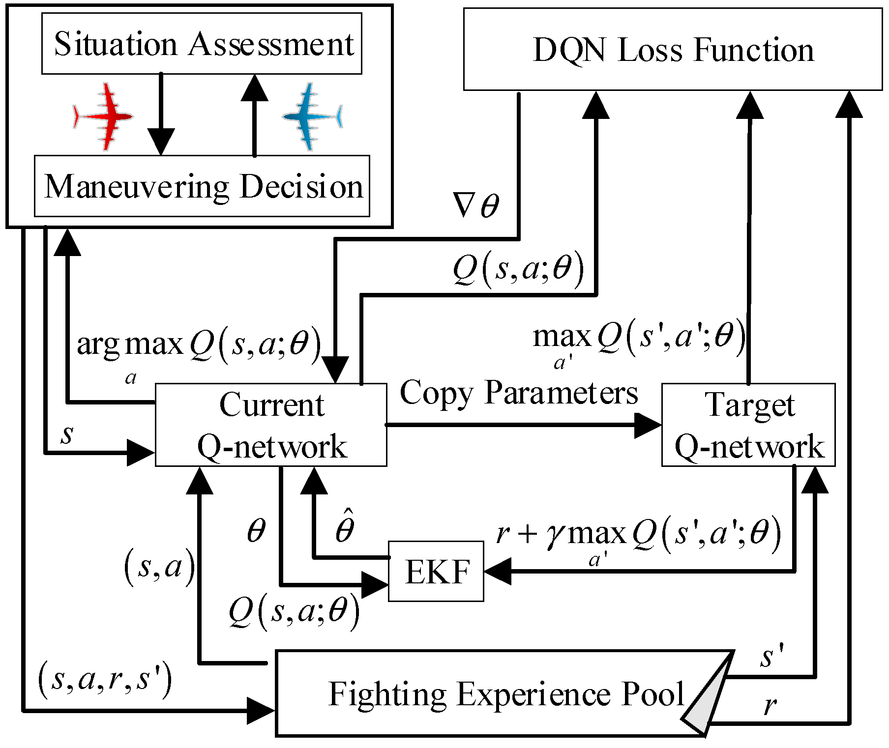
3. Deep Q-Network Hybridization with Extended Kalman Filter

This chapter introduces the architecture of deep Q-network and deep Q-network hybridization with an extended Kalman filter based on the characteristics of autonomous maneuvering decisions based on the real-time generation of maneuvering commands for UCAVs in complex dynamic air environment and gives the framework of this fusion algorithm with one-to-one UCAV air combat maneuvering decision generation.

3.1. Deep Q-Network Description

Deep learning has excellent feature learning ability, while reinforcement learning has strong decision-making ability. Deep reinforcement learning combines the advantages of both, making it widely used in dynamic decision making, real-time predictions, and gaming. The basic framework of deep reinforcement learning is composed of agents and environments. The agent selects actions according to a certain strategy based on the current state and rewards, and the environment responds to this action and receives the next state and rewards. Agents optimize their strategies by continuously updating the value function to maximize cumulative rewards.

A deep Q-network is a classic deep reinforcement learning algorithm based on a value function, designed to approximate the Q function (state value function). The Google DeepMind team proposed DQN in a paper published by NIPS 2013 [15]. The most important contribution is to directly use the original state space as the input of the network, while the input features are not manually completed like traditional reinforcement learning implementations. Similarly, they can use the same architecture to train agents to play different Atari games and achieve leading results.

In traditional reinforcement learning, state values are usually stored in the Q table, and after each action, the Bellman equation is used to update the Q table.

$$Q{(s,a)}_{new}={Q(s,a)}_{old}+\alpha [r+\gamma \underset{a\text{'}}{\max }Q(s\text{'},a\text{'})-Q{(s,a)}_{old}]$$

(9)

where $\alpha$ is the learning rate between 0 and 1, $r$ is the reward in the current state, $\gamma$ is the discount factor, $s\text{'}$ is the next state, and $a\text{'}$ is an optional action for the next state.

However, when the state dimension is high, the Q table suffers from the dimensionality explosion problem. DQN uses a neural network to represent the Q function, with the input being the state and the output being the Q value of each action. Unlike supervised learning, how to train Q-network remains to be solved. DQN uses a target network to calculate the target Q value, which is a replica of the main network but is not frequently updated to maintain the stability of the target Q value. The target Q value that the network needs to predict is calculated as in Equation (10).

$$Q^{\pi }(s_t,a_t)=r+\gamma \underset{a\text{'}}{\max }{Q}^{\pi }(s\text{'},a\text{'};{\theta }^{-})$$

(10)

where ${\theta }^{-}$ is the parameter of the target Q-network.

Loss calculation refers to the loss function used in training the main Q-network, which measures the difference between the Q value output from the main Q-network and the target Q value. The commonly used loss function is the mean square error (MSE), as shown in (11).

$$L(\theta )=\frac{1}{2N}{\displaystyle \sum _{i=1}^N{[r_i+\gamma \underset{a\text{'}}{\max }{Q}^{\pi }(s_i\text{'},a\text{'};{\theta }^{-})-Q(s_i,a_i;\theta )]}^2}$$

(11)

where N is the number of samples in a batch, and $s_i$ and $a_i$ are the state and action of the i-th sample.

The gradient update process of DQN is shown in formula (12) below.

$${\nabla }_{\theta }L(\theta )=\frac{1}{N}{\displaystyle \sum _{i=1}^N[r_i+\gamma \underset{a\text{'}}{\max }{Q}^{\pi }(s_i\text{'},a\text{'};{\theta }^{-})-Q(s_i,a_i;\theta )]}{\nabla }_{\theta }Q(s_i,a_i;\theta )$$

(12)

The two key techniques of DQN include using a memory replay buffer to store and sample historical transfer data, to break the correlation between data, and improve data utilization and learning efficiency. The ε-greedy strategy is used to balance exploration and utilization, which means randomly selecting actions with a certain probability, otherwise choosing the current optimal action.

3.2. DQN-EKF Algorithm

The purpose of the target Q-network is to improve the stability of Q value estimation and avoid continuous changes in the target Q value caused by the update of the main network parameters, thereby affecting the convergence of training. The parameters of the target Q-network are periodically copied from the main network, ensuring that the target Q value does not fluctuate violently with each step of training, but slowly follows the changes of the main network.

The true values of the weight parameters of the deep Q-network may have some deviation or fluctuation from the values we train, which may come from factors such as noise in the training data, randomness of the optimization algorithm, and complexity of the network structure. The uncertainty of network parameters can affect the performance and stability of the network, so it is necessary to analyze and filter out the uncertainty of network parameters [16].

EKF is an extension of the Kalman filter, which can handle nonlinear system models and observation models, while the Kalman filter can only handle linear models [17]. In a deep Q-network, the goal is to learn a Q function, namely $Q(s,a;\theta )$. It can consider the network parameters as system states and the Q value as observation values and use EKF to perform Bayesian inference and update on the network parameters. The state equation and observation equation are as follows.

$$\left\{\begin{array}{l}{\theta }_t=f({\theta }_{t-1},{\omega }_{t-1})={\theta }_{t-1}+{\omega }_{t-1}\hfill \\ z_t=h({\theta }_t,v_t)=Q(s_t,a_t;{\theta }_t)+v_t\hfill \end{array}\right.$$

(13)

where $f(\cdot )$ and $h(\cdot )$ are the state functions and observation functions of nonlinear systems, respectively; ${\omega }_t$ is the process noise, which follows a normal distribution $N(0,Q)$; and $v_t$ is the measurement noise, which follows a normal distribution $N(0,R)$.

The Taylor expansion of the equations of state and observation is used to approximate the nonlinear system as a linear system so that the Kalman filter can be used. This linearization process is also the core of the EKF.

For the state equation, a first-order Taylor expansion of $f({\theta }_{t-1},{\omega }_{t-1})$ at the a posteriori estimate ${\widehat{\theta }}_{t-1}$ at the time of $t-1$ yields the following Equation (14).

$$f({\theta }_{t-1},{\omega }_{t-1})\approx f({\widehat{\theta }}_{t-1},0)+{\left.\frac{\partial f}{\partial \theta }\right|}_{{\widehat{\theta }}_{t-1}}({\theta }_{t-1}-{\widehat{\theta }}_{t-1})+{\left.\frac{\partial f}{\partial \omega }\right|}_{{\widehat{\theta }}_{t-1}}{\omega }_{t-1}$$

(14)

where ${\omega }_{t-1}$ is simplified to 0 and $f({\widehat{\theta }}_{t-1},0)\sim {\tilde{\theta }}_t$, ${\left.\frac{\partial f}{\partial \theta }\right|}_{{\widehat{\theta }}_{t-1}}$ and ${\left.\frac{\partial f}{\partial \omega }\right|}_{{\widehat{\theta }}_{t-1}}$ are the partial derivative matrices at ${\widehat{\theta }}_{t-1}$ and 0, respectively. Approximating the above expansion formula into the state equation yields Equation (15).

$${\theta }_{\mathrm{t}}=f({\widehat{\theta }}_{t-1},0)+{\left.\frac{\partial f}{\partial \theta }\right|}_{{\widehat{\theta }}_{t-1}}({\theta }_{t-1}-{\widehat{\theta }}_{t-1})+{\left.\frac{\partial f}{\partial \omega }\right|}_{{\widehat{\theta }}_{t-1}}{\omega }_{t-1}$$

(15)

Equation (15) can be viewed as a linear system, where ${\left.\frac{\partial f}{\partial \theta }\right|}_{{\widehat{\theta }}_{t-1}}$ is the state transfer matrix, usually denoted $A$, and ${\left.\frac{\partial f}{\partial \omega }\right|}_{{\widehat{\theta }}_{t-1}}$ is the process noise matrix, usually denoted $W$.

For the observation equation, a first-order Taylor expansion is performed for $h({\theta }_t,v_t)$ at ${\tilde{\theta }}_t$, as shown in (16).

$$h({\theta }_t,v_t)\approx h({\tilde{\theta }}_t,0)+{\left.\frac{\partial h}{\partial \theta }\right|}_{\tilde{\theta }}({\theta }_t-{\tilde{\theta }}_t)+{\left.\frac{\partial h}{\partial v}\right|}_{\tilde{\theta }}{v}_t$$

(16)

where $v_t$ simplifies t to 0 and makes $h({\tilde{\theta }}_t,0)$ equal to ${\tilde{z}}_t$. ${\left.\frac{\partial h}{\partial \theta }\right|}_{\tilde{\theta }}$ and ${\left.\frac{\partial h}{\partial v}\right|}_{\tilde{\theta }}$ are the partial derivative matrices at ${\tilde{\theta }}_t$ and 0, respectively. Approximating the above expansion formula into the equation of state yields Equation (17).

$$z_t=h({\tilde{\theta }}_t,0)+{\left.\frac{\partial h}{\partial \theta }\right|}_{\tilde{\theta }}({\theta }_t-{\tilde{\theta }}_t)+{\left.\frac{\partial h}{\partial v}\right|}_{\tilde{\theta }}{v}_t$$

(17)

Equation (17) can also be regarded as a linear observation model, where ${\left.\frac{\partial h}{\partial \theta }\right|}_{\tilde{\theta }}$ is the observation matrix, usually denoted as $H$, ${\left.\frac{\partial h}{\partial v}\right|}_{\tilde{\theta }}$ is the observation noise matrix, usually denoted as $V$.

Therefore, using linearization, the state and observation equations obtained by linearizing at the posteriori estimate can be written in the following form:

$$\left\{\begin{array}{l}{\theta }_{\mathrm{t}}={\widehat{\theta }}_{\mathrm{t}}+A_{t-1}({\theta }_{t-1}-{\widehat{\theta }}_{t-1})+W_{t-1}{\omega }_{t-1}\hfill \\ z_t={\tilde{z}}_t+H_t({\theta }_t-{\tilde{\theta }}_t)+V_t{v}_t\hfill \end{array}\right.$$

(18)

where $p(W\omega )\sim N(0,WQ{W}^T)$, $p(Vv)\sim N(0,VR{V}^T)$.

After linearization, the process is divided into prediction and correction stages according to the method of linear Kalman filter.

In the prediction process, prior estimates need to be obtained for ${\widehat{\theta }}_{t^{-}}$, given by the system. Then, it is necessary to calculate the covariance matrix $P_{t^{-}}$ of the prior error $e_{t^{-}}$, as shown in (19).

$$P_{t^{-}}=A{P}_{t-1}{A}^T+WQ{W}^T$$

(19)

During the calibration process, the first step is to calculate the Kalman gain $K_t$ representing the proportion of the covariance of state observation prediction error to the covariance of observation prediction error; the calculation formula is as shown in (20).

$$K_t=P_{t^{-}}{H}^T{(H{P}_{t^{-}}{H}^T+VR{V}^T)}^{-1}$$

(20)

And then the posterior estimation of ${\widehat{\theta }}_t$ is calculated as (21).

$${\widehat{\theta }}_t={\widehat{\theta }}_{t^{-}}+K_t[z_t-h({\widehat{\theta }}_{t^{-}},0)]$$

(21)

Finally, it is necessary to update the covariance matrix $P_t$ of the state estimation error $e_t$, as shown in (22).

$$P_t=(I-K_{t}H)P_{t^{-}}$$

(22)

To summarize the above formula, the algorithm flow of combining DQN and EKF is mainly as follows (Figure 2):

Step 1: 

Initialize the deep Q-network model, parameters, and its covariance matrix $P_0$.

Step 2: 

For each time step $t=1,2,\dots$, perform the following sub-steps:

(i) 

Prediction: Based on the state transition equation and process noise, predict the mean of state ${\widehat{\theta }}_{t^{-}}$ for the next time step and covariance $P_{t^{-}}$.

(ii) 

Correction: Calculate the Kalman gain $K_t$ based on the observation equation and observation noise and update the mean of state ${\widehat{\theta }}_t$ and covariance $P_t$.

(iii) 

Interaction: Based on the current state observation $s_t$ and the ε-greedy strategy, select an action $a_t$ and execute it using the main network $Q(s_t,a_t;{\widehat{\theta }}_t)$ with the optimal true parameter estimates to obtain the reward $r_t$ and the next state $s_{t+1}$.

Step 3: 

Repeat the above steps until the convergence condition is met or the maximum number of iterations is reached.

In summary, the system state is the weight of DQN, the system dynamic model is DQN itself, and the observation model is the function H that maps the weight to the Q value. EKF is used to handle nonlinear situations and consider the uncertainty of weights and observations. The network parameters updated through EKF iteration are calculated based on the formula of the Kalman filter (KF). KF is an optimization method used to estimate system state, which continuously updates the posterior distribution of the state using the dynamic model and observation model of the system. The network parameters updated after EKF iteration will be closer to the true values and have less uncertainty.

4. Simulation Experiments

4.1. Simulation Experiments Design

To verify the effectiveness of the DQN hybridization with EKF algorithm proposed in this article in solving the autonomous maneuvering decision generation problem of UCAVs, simulation experiments’ design and analysis will be described in this section.

The hardware used in this simulation is Intel(R) Core (TM) i9-12900H CPU with 32 G RAM and NVIDIA GeForce RTX 3060 GPU. Operating system and software versions are Windows 64-bit, torch1.13.1 + cu117, python 3.9.16, and MATLAB 2022b.

Before the simulation starts, it is necessary to initialize the air combat environment and assign the starting positions and movement directions of the red and blue sides according to the requirements of the adversarial task, followed by adversarial simulation training. Among them, the maneuvering strategy of our UCAV always relies on the hybridization algorithm of DQN-EKF for decision making. We are assuming that the scope of the air combat environment is limited to a cube with a side length of 12 km. Assuming the performance of both red and blue aircraft is consistent, with a maximum flight speed of 400 m/s, close to Mach 1.2, a stall speed of 180 m/s, and a maximum normal overload of 8 G. The maneuver decision cycle is set to 0.25 s, which means that every 0.25 s, both red and blue aircraft have an opportunity to select maneuver actions based on the current air situation. In addition, the rules for determining victory or defeat are, within the limited number of maneuver decision steps, if our unmanned fighter’s attack angle is less than 60° and escape angle is less than 30°, and our continuous dominance in this attack range reaches 9 times or more times, our victory will be determined. On the contrary, the enemy wins, otherwise, it is a draw.

During the simulation training phase, an online learning process will be conducted for 6000 rounds of confrontation between the red and blue sides, with a maximum simulation step count of 250 in each round, which is close to one minute of autonomous maneuvering combat time.

Table 1. Parameters setting for DQN.

Index	Value
memory capacity	20,000
discounted factor	0.9
batch size	64
learning rate	0.008
ε-greedy value	0.95–0.01

below provides the key parameter settings for DQN.

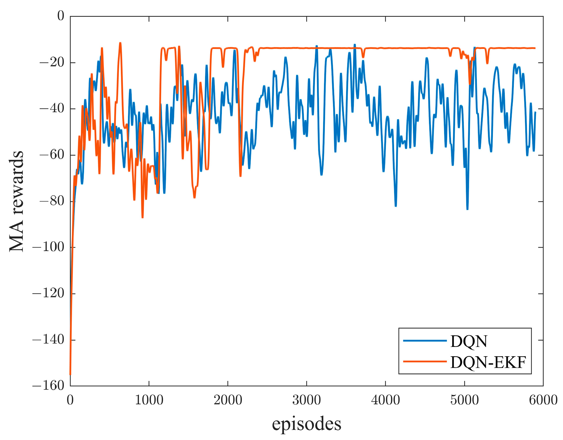
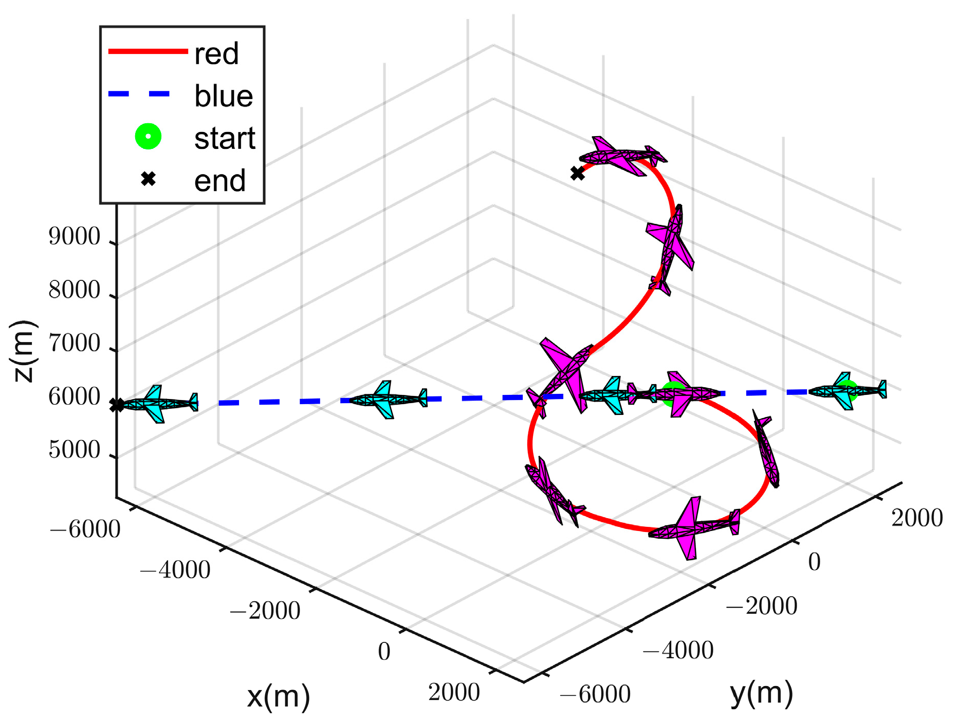
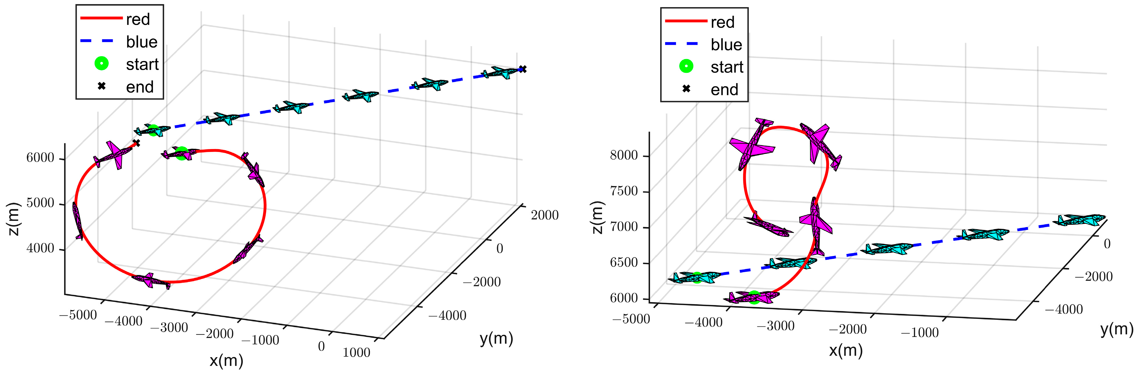
4.2. Simulation Experiment Analysis

In actual one-on-one air combat, pilots will control the aircraft’s joystick based on the occupancy information of both the enemy and ourselves. In order to achieve autonomous maneuver decision generation for UCAVs, it is necessary to rely on intelligent decision-making networks to make maneuvering action choices after analyzing the air combat environment situation. Conducting simulation experiments is a low-cost verification method. Designing different initial air combat situations directly affects the generation of maneuver decisions. Before the start of the simulation experiments, a confrontation scenario in which both sides are at a disadvantage is designed to approximate the actual air combat engagement process.

The UCAVs of the red and blue sides are in a state of balance, representing mutual checks and balances. In the initial stage, both red and blue are flying at the same speed and the same altitude. But their initial flight heading is in the same straight line and opposite direction, which is a state of head-on flight.

Following the pre-defined network parameters and air combat environment design, the integrated reward curve for the rounds obtained by our UCAV throughout the training process is shown in Figure 3. The figure clearly shows that as the training is iterated, the reward value has a rapid increase compared to the starting phase. Compared to the traditional DQN, the DQN-EKF method of training rewards can be highly rewarding and the reward values are more stable in the later stages of training. By calculating the cumulative average reward for each episode, the original DQN score was −25.05, and now the DQN-EKF score is −42.31. DQN-EKF has a numerical improvement of 68.90%. The training results demonstrate the feasibility of the DQN-EKF in solving the autonomous maneuvering decision generation problem for UCAV.

When the red and blue sides are at a disadvantage to each other, ideally the red aircraft should increase the angle factor, altitude factor, and speed factor to gain a greater energy advantage and battlefield initiative. Therefore, the following is a review and analysis of the flight trajectories of the red and blue sides, and two representative maneuvering decision trajectories are selected for discussion.

(I) 

Strategy 1

Figure 4 shows the course of the fight trajectory of the red and blue sides. Due to the head-on attitude in the initial phase, if the red UCAV does not take any maneuvering action and still maintains its initial maneuvering action, it increases the risk of being shot down by the blue UCAV. Therefore, the red side makes a rightward circling flight in the initial phase to avoid the possibility of being shot down. When the distance between the two sides is close, the red UCAV makes a maneuver with the tendency to attack, and then pulls upwards to expand its advantage in altitude and make the accumulation of potential energy. Finally, the red UAV successfully enters the rear of the attack target and keeps it within its own attack range. Figure 5 shows the trend of attack angle and escape angle of the red and blue UCAVs. Towards the end of the round, the attack angle of the red UCAV converges to zero after several adjustments. At the same time, the fleeing angle is also stable and close to zero. This indicates that the red side is in a more stable attack zone and the blue side is in a non-escapable zone.

(II) 

Strategy 2

Strategy 2 shows the flight trajectories of the red and blue sides as shown in Figure 6. In this round of air combat fighting, the maneuvering decisions of the red unmanned fighters are shown to be very simple. Their angle of attack and angle of escape changes during the engagement are shown in Figure 7. The red unmanned fighter’s heading makes a change out to the left from the initial moment, which can be roughly seen as a pull-up to the upper left. This maneuver effectively parries the target weapon attack, while completing the accumulation of its own attack advantage. Subsequently, the red unmanned fighter dives and turns at an altitude of about 7 km to adjust its attitude and create attack conditions until the blue unmanned fighter shoots it down. Compared with the maneuver decision process of the strategy, this strategy appears to be more efficient and takes fewer maneuver steps. The above maneuver decision strategy also laterally reflects the reliability of the maneuver decision network trained by the DQN and EKF hybrid algorithms.

We continued to use the DQN-EKF hybrid algorithm to simulate the initial state of parallel flight between two UCAVs, which demonstrated the process of the red side accumulating its own advantages from the initial situation of equal strength between the two sides. The red side UCAV first dives downward, completing a circle of vertical mediation to form a tail chase situation. But the trajectory on the right of Figure 8 shows the opposite, with the red side launching attacks from above enemy aircraft.

5. Conclusions

The maneuver decision-making method based on deep Q-network hybridization with an extended Kalman filter proposed in this article can achieve truly autonomous maneuver decision-making for UCAVs. This method combines the advantages of a deep Q-network in solving the game problem and the ability of an extended Kalman filter in solving the uncertainty of network parameters. By analyzing the results of the DQN-EKF network training, it can be found that the method used in this paper can have faster convergence than the original DQN. The average reward of the DQN-EKF hybrid algorithm is 68.90% higher than the original DQN algorithm. Due to the addition of EKF, the optimal true parameter estimates are obtained by continuous iterative updates, and the optimal true parameter estimates are used to calculate the accurate maneuver value function and select the optimal maneuver decision maneuver. The flight trajectories of the simulation experiments show that the maneuver strategy generated by this method can enable the UCAV to perform the task of defeating enemy aircraft more autonomously, accurately, and stably in a dynamic 3D environment and complete the autonomous maneuver decision. Future research will target the design of a hybrid parallel computing framework to make improvements in the efficiency of training.

References

1. Byrnes, M.W. Nightfall: Machine autonomy in air-to-air combat. Air Space Power J. 2014, 28, 48–75. [Google Scholar]
2. Sun, Z.; Yang, S.; Piao, H.; Chen, C.; Ge, J. A survey of air combat artificial intelligence. Acta Aeronaut. Astronaut. Sin. 2021, 42, 35–49. [Google Scholar]
3. Jordan, J. The future of unmanned combat aerial vehicles: An analysis using the Three Horizons framework. Futures 2021, 134, 102848. [Google Scholar] [CrossRef]
4. Hambling, D. AI outguns a human fighter pilot. New Sci. 2020, 247, 12. [Google Scholar] [CrossRef]
5. Virtanen, K.; Raivo, T.; Hamalainen, R.P. Modeling Pilot’s Sequential Maneuvering Decisions by a Multistage Influence Diagram. J. Guid. Control Dyn. 2004, 27, 665–677. [Google Scholar] [CrossRef]
6. Smith, R.E.; Dike, B.A.; Ravichandran, B.; El-Fallah, A.; Mehra, R.K. Two-Sided, Genetics-Based Learning to Discover Novel Fighter Combat Maneuvers. Comput. Methods Appl. Mech. Eng. 2000, 186, 421–437. [Google Scholar] [CrossRef]
7. Deng, K.; Peng, X.; Zhou, D. Study on Air Combat Decision Method of UAV Based on Matrix Game and Genetic Algorithm. Fire Control Command Control 2019, 44, 61–66. [Google Scholar]
8. Li, S.; Ding, Y.; Gao, Z. UAV air combat maneuvering decision based on intuitionistic fuzzy game theory. Syst. Eng. Electron. 2019, 41, 1063–1070. [Google Scholar]
9. He, X.; Jing, X.; Feng, C. Air Combat Maneuver Decision Based on MCTS Method. J. Air Force Eng. Univ. Nat. Sci. Ed. 2017, 18, 36–41. [Google Scholar]
10. McGrew, J.S.; How, J.P.; Williams, B.; Roy, N. Air-Combat strategy using approximate dynamic programming. J. Guid. Control Dyn. 2010, 33, 1641–1654. [Google Scholar] [CrossRef]
11. Du, P.; Liu, H. Study on air combat tactics decision-making based on Bayesian networks. In Proceedings of the 2010 2nd International Conference on Information Management and Engineering, Chengdu, China, 16–18 April 2010; pp. 252–256. [Google Scholar]
12. Ji, H.; Yu, M.; Yang, J. Research on the Air Combat Countermeasure Generation of Fighter Mid-Range Turn. In Proceedings of the 2018 2nd International Conference on Artificial Intelligence Applications and Technologies (AIAAT2018), Shanghai, China, 8–10 August 2018; pp. 522–527. [Google Scholar]
13. Xu, J.; Guo, Q.; Xiao, L.; Li, Z.; Zhang, G. Autonomous Decision-Making Method for Combat Mission of UAV based on Deep Reinforcement Learning. In Proceedings of the 2019 4th Advanced Information Technology, Electronic and Automation Control Conference (IAEAC), Chengdu, China, 20–22 December 2019; pp. 538–544. [Google Scholar]
14. Pope, A.P.; Ide, J.S.; Micovic, D.; Diaz, H.; Rosenbluth, D.; Ritholtz, L.; Twedt, J.C.; Walker, T.T.; Alcedo, K.; Javorsek, D. Hierarchical Reinforcement Learning for Air-to-Air Combat. In Proceedings of the 2021 International Conference on Unmanned Aircraft Systems (ICUAS), Athens, Greece, 15–18 June 2021; pp. 275–284. [Google Scholar]
15. Mnih, V.; Kavukcuoglu, K.; Silver, D.; Graves, A.; Antonoglou, I.; Wierstra, D.; Riedmiller, M. Playing Atari with Deep Reinforcement Learning. arXiv 2013, arXiv:1312.5602. [Google Scholar]
16. Srichandan, A.; Dhingra, J.; Hota, M.K. An Improved Q-learning Approach with Kalman Filter for Self-balancing Robot Using OpenAI. J. Control Autom. Electr. Syst. 2021, 32, 1521–1530. [Google Scholar] [CrossRef]
17. Mohammaddadi, G.; Pariz, N.; Karimpour, A. Extended modal Kalman filter. Int. J. Dyn. Control 2017, 19, 728–738. [Google Scholar] [CrossRef]
Figure 1. Spatial geometric relationship for UCAVs.
Mathematics 12 00261 g001
Figure 2. DQN-EKF Algorithm Block Diagram.
Mathematics 12 00261 g002
Figure 3. Trend chart of episode rewards.
Mathematics 12 00261 g003
Figure 4. Flight trajectory in strategy 1.
Mathematics 12 00261 g004
Figure 5. Angle of attack and escape variation curves in strategy 1.
Mathematics 12 00261 g005
Figure 6. Flight trajectory in strategy 2.
Mathematics 12 00261 g006
Figure 7. Angle of attack and escape variation curves in strategy 2.
Mathematics 12 00261 g007
Figure 8. Different flight trajectory in parallel flight dilemma.
Mathematics 12 00261 g008