1. Introduction
In the context of manufacturing companies, production planning and control (PPC) plays a crucial role in achieving the desired production quality and rate while also preventing potential disruptions [
1]. One of the most significant disruptions that can affect system efficiency is machine failure, which often results from gradual and irreversible damage that accumulates over time during operation, commonly referred to as “soft failures” [
2]. Failure to accurately predict or analyze faults can result in substantial costs associated with production downtime and material waste [
3]. One key challenge in accurately identifying and predicting machine failures is incomplete or incorrect modeling and identification of underlying machinery degradation [
4]. To address this problem, researchers have explored and developed various methods of degradation identification, such as physics-based models, data-driven models, and hybrid models, to estimate the state of health (SoH) and predict the remaining useful life (RUL) of machines.
The results obtained from these estimates and predictions are crucial for optimizing maintenance planning and high-level policy making [
5]. Various studies, including [
6,
7], have proposed methodologies for optimizing maintenance planning based on SoH estimation for systems with different topologies. Other methods, such as those developed by [
8,
9], rely on the predicted RUL for maintenance-planning-optimization purposes. However, the applicability of these approaches in real-world scenarios may be limited because PPC optimization requires information about the unique physical characteristics and working conditions of field machines and some degree of control over the degradation of the machines. Nonetheless, most research on high-level-maintenance policy-making methods uses generic mathematical models for the system as a whole, without taking into account the system’s physical characteristics, including all of its subsystems and their various operating conditions [
10,
11].
Merely considering production planning from a high-level perspective is insufficient because making informed high-level decisions requires insight into low-level operations. To address this gap, an alternative approach that optimizes production and maintenance has been adopted, grounding itself in the reliability analysis of machinery at the operational level. However, these methods face challenges similar to those encountered by high-level planning strategies. Specifically, three factors make the majority of current methodologies incompatible with high-level decision-making processes, thereby limiting their effectiveness in supporting planning decisions on the shop floor. First, creating a physical model to depict system degradation is a costly task, and although it provides accuracy and physical interpretability, it makes the resulting techniques exclusive and expensive [
12,
13,
14,
15,
16]. Second, the assumption that the deterioration of a system can be accurately modeled using predetermined physical or mathematical models is wrong. This is because the degradation of different components within the system may follow unique paths or not conform to well-established or closed-form mathematical models [
17,
18]. Third, using data-driven methods can lead to a loss of connection to the physical structure of the system, resulting in significant information loss about the nature of the degradation and eventual failures [
19,
20].
The lack of integration between high-level and low-level perspectives in production and maintenance optimization highlights a significant gap. Neither approach, when applied in isolation, has successfully established a comprehensive link for the joint optimization of production and maintenance in a generalized manner. Consequently, a universal method for optimizing PPC based on the system’s SoH remains elusive. This disconnect results in maintenance planning for PPC optimization being largely reliant on estimations and predictions. It limits the ability to support strategic decisions at the shop-floor level, such as mitigating failures or managing the types of failures that occur. These decisions require an understanding of the system’s physical properties and the ability to control system degradation, which most existing methods cannot provide without the substantial investment required for physical modeling. Therefore, there is an evident demand for cost-effective strategies that can accommodate the distinct physical attributes of each system and its operational conditions, to aid in making informed high-level decisions.
To address this issue, a number of research studies have been published on methods for extending the life of machines, focusing on soft failures rather than hard failures, and utilizing physically interpretable degradation data. For instance, the study in [
21] introduced an innovative method to achieve a balance between reliability and performance in control systems with degrading actuators. This was accomplished through a dynamic model-predictive-control framework, which included the modeling of actuator degradation. Similarly, the works in [
22,
23] proposed strategies to prolong machine lifespan by recognizing actuator degradation as one of the system states. Nonetheless, a common limitation of these methodologies is their reliance on a predefined physical model to describe the degradation process. Additionally, the study in [
24] detailed a novel approach that integrates machine learning with reliability-centered maintenance, to rank industrial assets for life-extension interventions based on condition-monitoring data. The research in [
25] focused on developing a dynamic-optimization framework aimed at improving both the lifespan and economic efficiency of Li-Ion-battery-energy storage systems by incorporating battery health into the operational decision-making process. Furthermore, ref. [
26] proposed a machine-learning-driven decision-making model for extending the life of industrial assets. This model synergizes reliability-centered maintenance, condition monitoring, and prognostics and health management strategies.
While these studies aimed to enhance the longevity of machinery and to bridge the gap between high-level decisions and low-level actions, two significant practical challenges persist. Firstly, to manage degradation, these approaches typically rely on predefined mathematical models or define the degradation process through differential equations, to integrate it as a controllable state within the system model. This reliance on specific assumptions introduces limitations and raises concerns about the method’s applicability, including issues related to controllability and observability. Secondly, some strategies aimed at prolonging machine lifespan emphasize maintenance or operational changes rather than concentrating on controlling the degradation of individual machines. While beneficial for specific scenarios, this approach generally has a considerable effect on production. Consequently, optimizing the system’s performance becomes exceedingly complex, complicating the feasibility of their practical implementation.
Thus, the main question to answer is whether it is possible to identify the degradation in any system in a physically interpretable manner without using predefined mathematical models or paying the high price of physical modeling. In this way, it becomes possible to control the reliability of the machines and to support high-level decisions to keep machines operational until the desired time of maintenance. To this end, this article proposes a method that, instead of physically modeling the system and its degradation, estimates the effect of every system action on its SoH, based on historical data. This method of degradation identification is based on machines’ unique characteristics and working conditions and is also physically interpretable. This will eventually offer the possibility of optimization of PPC and maintenance planning by providing the ability to regulate machine maintenance using the degrading effect that each action of the machine has on its SoH. Additionally, being able to control the degradation means the accuracy of the RUL prediction will increase dramatically and, eventually, the goal of maintenance planning will only be to choose the best degradation rate for the machine, so that the best compromise between production cost and maintenance cost becomes achievable.
The primary goal of this research was to develop degradation-aware systems. These systems are designed from a standalone controller perspective, enabling them to make informed decisions to preserve the machine’s output quality and manage its lifespan. This objective was pursued without relying on predefined assumptions about the degradation model or the system’s operating conditions, aiming for a smarter and more adaptable approach to system maintenance and longevity. In this way, the existing gap in the field, between high-level maintenance planning and low-level machine control for maximum flexibility, would be filled by proposing a closed-form control policy based on the empirical degradation model.
To this end, this article proposes a general method for controlling low-level actions in machines according to the maintenance policy. This method was designed by altering the quadratic cost function of the optimal control and by including the degradation cost in the control strategy. The main examples used with this method are increasing the machine’s mean time to failure (MTTF) by controlling the actions that have a more severe effect on degradation and eventual loss of control.
For this reason, first, the cost of each machine’s action based on the SoH is calculated. This method does not consider any predefined model for the degradation, and it makes no assumption about the working conditions. Then, a control method based on a linear–quadratic regulator (LQR) is proposed, so that the machine can optimally control the output according to the SoH.
The outline of this article is as follows. The methods for SoH-aware controllers will be proposed in
Section 2. In
Section 3, the methods and material used for the simulation to validate the proposed method will be discussed. In
Section 4, results from the simulation will be shown and validated. The main pros and cons of the proposed method will be discussed in
Section 5.
Section 6 will be the conclusion.
2. Methods
This section will present a comprehensive analysis of the various techniques employed in designing the linear–quadratic degradation controller (LQDR). The first part will outline how the degradation can be recognized as a function of the system’s states and actions, without resorting to physical modeling. The second part will put forth an optimal feedback mechanism that effectively regulates the rate of degradation within the system, thereby enhancing its reliability and availability.
The assumptions for this problem are as follows:
The system model is available and linear.
The record of the system input(s) and output(s) are available with or without state-estimation techniques (the system must be observable and controllable).
The record of the failure time is available.
2.1. Control Criteria
According to [
27] and
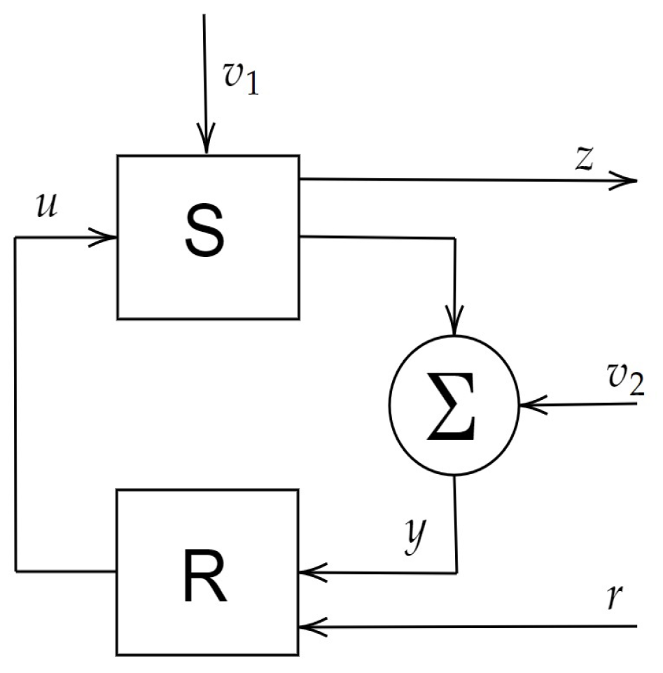
Figure 1, the definition of a control problem is: “given a system S with a measured output signal
y, determine a feasible control input
u, so that controlled variable
z as closely as possible follows a reference signal (or set point)
r, despite the influence of disturbance
, measurement error
, and variations in the system”, where
R is the controller.
Multiple cost functions can be formulated by considering the desired output precision and system characteristics to solve the control problem. Subsequently, the optimal-control problem can be defined as the process of minimizing the cost function, such as a quadratic cost:
where
is the error and
and
are penalties for the error and input signal, respectively [
28].
Considering that wear, corrosion, deformation, and fracture, which are physical phenomena happening only during the operation of systems, constitute the components of degradation (the deterioration of an inactive machine does not present a concern for predictive maintenance), it can be inferred that the degradation model and rate of a machine are inherently correlated with the decisions and actions taken by the controller. This relationship highlights the significance of effective control strategies in the preservation of machine health and the subsequent optimization of system performance.
In the context of Industry 4.0, it has become feasible to employ advanced techniques such as big-data analysis and machine learning to predict the impact of each decision or action of the machine on any system’s parameters. Examples of such parameters include the impact of elevated torque on gearbox degradation, which can subsequently be utilized to regulate the SoH; the impact of high current consumption on battery state of charge, which can subsequently be utilized to regulate the state of charge (SoC); and the cost associated with delayed delivery relative to the low angular velocity of the motor working in the conveyor system, which can subsequently be utilized to optimize the maintenance policy [
29].
Therefore, through the redefinition of the cost function associated with the optimal-control problem, it becomes possible to optimize control actions not solely based on the output error and system input but also with consideration for additional desired factors, such as degradation.
Eventually, (
1) can be redefined as:
where
f can be any desired function depending on the optimization goal.
2.2. Optimality of Control
Consider the state-space model as the machine model for control,
where
x includes the system state(s),
u is the system input(s),
A and
B represent the nominal system’s parameters (considered constant in time-invariant systems),
C is the relationship between the output(s) and state(s) of the system,
N defines the relationship of the disturbances to the system states,
M defines the parameter(s) to control,
is the process disturbance, and
is the measurement noise.
Based on the optimal-control cost function presented in (
1), it is evident that each action is associated with a particular cost. Therefore, optimizing the system based on a cost function that includes additional factors beyond the system’s error and output, as demonstrated in (
2), introduces an extra cost to the computation process that can potentially alter the optimality criteria and render the optimal point of (
1) suboptimal. As a consequence, the output of the system is highly likely to be impacted. This change in the output represents the cost incurred for reducing the system’s degradation rate.
The constraints imposed by control systems necessitate that the cost associated with degradation control can solely be paid via one of the following forms: more energy consumption, reduction in output quality, reduction in output rate, or degradation sharing (load sharing). The choice of the particular parameter to be adjusted as compensation for the degradation control cost is based upon the interrelationships among the quantities of
,
, and
as depicted in (
2).
Taking into account (
2) as the designated objective function for minimization, the penalty matrices, denoted as
,
, and
, serve to present the production priorities and effectively map high-level decisions to corresponding field machine actions. In this way,
conveys the relative significance of the final product quality,
quantifies the significance of the input utilization costs, and lastly,
reflects the criticality of preserving the system health.
Controlling the production priorities by utilizing these penalty values can be elucidated more effectively through an illustrative example. Rolling mills are important in the steel industry as they facilitate the production of steel in accordance with specific requirements. However, irrespective of the quality of the final steel product, a market demand persists for it. Further clarity can be gained by considering three distinct scenarios.
The first scenario involves a situation where the utmost emphasis is placed on the quality of the final product, and production batches are ordered with a specific objective. In this context,
is chosen to have a very high value. Consequently, the production cost
J in (
2) becomes highly sensitive to any deviation of the final product quality from the desired standards. As a result, the controller strategically allocates other resources (comprising the other two terms in (
2)) to minimize
J as much as possible.
The second scenario is when there is a substantial increase in energy costs, necessitating scrupulous conservation of energy usage during production. In this case, it becomes imperative to assign a high value to the parameter . As a result, the controller is granted the flexibility to lower the output quality and/or subject the system to greater degradation, all in the pursuit of minimizing energy consumption and thereby keeping J at a minimum.
Lastly, the third scenario arises when there is a delay in the delivery of a spare part or a shortage of maintenance staff for a certain period. In such instances, it is prudent to increase the value of the parameter . By doing so, the production policy of extending the machine’s lifetime can be followed. Consequently, the controller is authorized to increase the energy usage and/or compromise the output quality to achieve the objective of extending the machine’s operational lifespan.
By considering these three scenarios within the context of a rolling mill, it becomes apparent how the selection of values for , , and can effectively translate production priorities into maintenance activities for the field machines. This allows for precise control of production and maintenance planning in accordance with the established priorities.
Upon establishing the system’s model and the degradation control cost-payment method, using the penalties relationship, the state–action cost (SAC), denoted as
f in (
2), should be computed.
2.3. State–Action Cost Calculation
Unlike the first and second terms of (
2) that depend solely upon output error (first term) or input to the system (second term), the third term, degradation, is potentially a function of both the input(s) and the state(s) of the system:
In order to effectively control the degradation, it is imperative to compute the cost of each state–action pair, which can be subsequently employed in the generation of the function f.
A universal approach that can be applied to any system, irrespective of its structure and operating conditions, involves the computation of costs associated with every possible combination of state–action pair. This calculation is based on historical system-failure data. Assuming that the machine is in a healthy state following each maintenance activity, a vector denoted by
can be formulated. This vector represents the costs of all feasible state–action combinations:
where
n is the number of all possible (combinations of) system states,
m is the number of all possible (combinations of) system actions, and
k is the number of all possible system state–action combinations. Define
S as a vector including the number of times that each of the members of
is repeated in one run-to-failure record,
and define
as a matrix including
N run-to-failure records, (
)
Then, the cost of each state–action combination from the degradation viewpoint can be calculated using
where
L can be any positive constant.
In the context of optimization as described in (8), the system’s SoH is modeled as a reservoir with a capacity of
L. This reservoir is replenished to full capacity following each maintenance event and depleted to empty with each system failure. Through the application of (
8a), a specific cost is allocated to each state–action pair, reflecting the quantity of the SoH consumed by the action. Consequently, every action depletes a portion of the system’s health. Given the absence of any state–action pair capable of enhancing the system’s health, (8b) incorporates this constraint into the computation. The optimization process is entirely reliant on the records of the system’s input and output, without taking into account the structure of the system itself. Moreover, given that the system being analyzed operates in a closed-loop manner, access to its input and output is deemed sufficient for the study.
To construct the function
as described in (
5), it is necessary to perform a quantization of the system’s states and actions. The level of quantization required is determined by the desired accuracy of the degradation control. In situations where the desired output of the system has only a small number of distinct settings, the number of combinations of states and actions will be limited and can be handled easily. Conversely, in systems with a continuous interval of desired output values or a large number of possible states, constructing
may not be feasible.
Function estimators are the most effective solutions for addressing this issue, and various linear and nonlinear regression techniques can be employed for this estimation. However, neural networks and relevance vector machines are the most appropriate function estimators for this task, due to the unsmooth nature of the SAC function. To utilize function estimators, a limited number of state–action combinations can be used to construct . The outcomes of (8) can be used to train a function estimator. Finally, the trained function estimator can eventually estimate the entire spectrum of .
2.4. Linear–Quadratic Control
Now that the SAC of the system is calculated, it is possible to design the controller based on the minimization of (
4). An LQR is an optimal controller designed based on the state space. The quadratic criterion that the LQR minimizes is (
1). The optimal-control signal for this controller can be written as follows [
27]:
The optimal feedback gain is then calculated by solving
subjected to a discrete Riccati equation,
The stability of the LQR is ensured by two key conditions: firstly, the system must be linear and, secondly, the system must be observable and controllable. When these conditions are met, the feedback matrix L derived from the control strategy is optimal, based on the specified penalty matrices.
The LQR optimizes the control problem for the infinite horizon, which means that the optimal feedback gain stays the same regardless of the inputs and outputs throughout the system’s lifetime. However, as the system’s parameters are time-variant (considering degradation), the actual system parameters deviate from the nominal values employed in designing the controller. Such deviations, over time, lead to a reduction in the control quality of the controller. Ultimately, when the deviation between the desired and actual output surpasses a predetermined threshold, the system is deemed to have failed [
30].
To be able to control the degradation for an infinite horizon, the SAC should be assumed as a smooth function and should be defined as a linear function of the state(s) and action(s),
where
and
are row vectors including the effects of state–action
on the system’s degradation. Regardless of the number of states and input,
f will always be a vector with two rows. The first row is the effect of the states on the degradation, and the second row is the effect of the input on the degradation. As the
is already calculated,
and
can be calculated by minimizing
Then, using the calculated
W from (14), it is possible to generate
f in (
4) and minimize it as the cost function of the optimal degradation control. In this case, the optimization problem is
(For for better readability in this section only, the apostrophe “′” is used instead of “T” to show the matrix transpose.)
Theorem 1. The optimal feedback that minimizes the cost function in (15)
iswhere L is calculated according to (
11)
, but in order for L to be optimal according to cost function (15)
, which includes degradation terms, S must be calculated usinginstead of solving (
12)
. The Schur vectors span the stable deflating subspace [31,32,33], and they are the results of the decomposition of Z in the form ofand Z iswhere This approach integrates degradation cost into the feedback control loop alongside error and input costs. This stands in contrast to S computed by solving (
12)
, which only considers error and input costs. Proof. Using the Lagrange multiplier, optimization of (15) becomes
The optimal solution can be found using the derivative of the cost function equal to zero:
Then solving for
u from (
26b):
Substituting
u derived from (
27) in (
26a) and (
26c) gives
Matrix
Z can be generated using (
28) and (
29):
For
x and
in (
30) to converge to zero as
,
Z must be stable. This can be done using eigen decomposition of the calculated
Z and generating the Schur vectors
according to (
18). Using the Schur vectors
S computed from the generated data, as depicted in (
17), and incorporating them into (
11), ensures both stability and the integration of degradation within the feedback loop. The stability criteria for the proposed method align with those of the LQR. Stability is assured as long as the system remains linear and all states are accessible, whether directly observed or estimated through state-estimation techniques. □
3. Simulation
The proposed techniques underwent validation via a simulation model. The primary objective of the simulation was to demonstrate the controller’s ability to regulate machine degradation and respond to changes in the system’s physical parameters resulting from degradation, thereby increasing the MTTF by keeping the output quality inside the desired threshold for a longer time. The methodology employed for the degradation simulation was designed to simulate the actual degradation process in a system.
To be able to focus on the control policy of the proposed controller, two distinct degradation models were defined. Each model was designed to elicit divergent responses from the controller, thereby enabling an assessment of the efficacy of the new optimization criterion. This will be explained further in the next section when the degradation models are discussed.
The device utilized in this simulation was a DC motor, which was favored for its simple design and reliable performance across diverse applications. A primary limitation of DC motors is the degradation of their internal parameters, particularly resistance, which can have significant consequences on the motor’s operation. Two processes account for changes in the internal resistance of DC motors. First, inter-turn short-circuiting as a result of insulation damage ultimately decreases the motor’s internal resistance over time [
34]. Second, the gradual wear of the brushes leads to a continuous decrease in motor resistance [
35]. When the controller is designed based on the nominal motor parameters, these changes in internal parameters due to degradation lead to deviations between the desired and actual output over time. Eventually, this deviation passes a certain threshold, and the system will be considered to have failed.
On some occasions, particularly in critical systems such as CNC machines for carving or pumps for 3D metal printing, minor discrepancies can have a significant impact on the final product, resulting in substantial costs due to energy and material wastage. Therefore, the primary objective of the simulation conducted to validate the method of degradation control was to demonstrate that, in spite of the variation in the nominal parameters of the motor, the LQDR diminished machine degradation and prolonged machine functionality compared to the LQR. The LQDR achieved this by precisely regulating the output during operation, ensuring that the system remained reliable throughout extended operations, in accordance with the desired outcome.
3.1. DC Motor Model
The state space of the DC motor can be written as [
36]
where
is the motor current,
is angular velocity,
is the resistance,
is the inductance,
is the back-emf,
is the torque constant,
is the motor inertia,
is the friction coefficient,
v is the input voltage, and
I is the identity matrix. In this system, voltage serves as the input, while current and angular velocity are the system’s states. Angular velocity is also utilized as the control variable.
3.1.1. Degradation Model
The working cycle was defined as the time period commencing from the initiation of the task execution by the machine until its cessation upon completion of the task. This temporal interval was denoted by
T. The two degradation models considered for this system were defined as [
37,
38]
where
c was the working cycle, and
defined the degradation model to be used. In this particular formulation, the reduction in motor resistance was modeled as a mathematical function of the cumulative summation of the exponent of the variations in both the input and state variables of the system. Thus, the degree of degradation experienced by the system was proportional to the sum of the magnitude of the changes occurring in the input and state variables. Furthermore, the steady-state degradation of the controller, wherein the input and state variables remained constant, was accounted for by incorporating a term equal to
into the formula.
The difference between the two models of degradation can be attributed to the extent to which changes in each of the states and inputs impacted the degradation of the system. In the first model (), the degradation of the system was influenced significantly more by changes in the states of the system, the angular velocity, and the current, as compared to the second model (), where the impact of the input on degradation had notably increased compared to the effects of the states that had decreased. This difference can be observed by comparing the coefficient matrices in Equations (32d) and (32e). Consequently, the LQDR needed to rationally compensate for the degradation caused by changes in the system states in the first model, in contrast to the second model, where the controller needed to compensate for the degradation caused mainly by changes in the input. Thus, the same controller structure needed to function in two distinct ways, based solely on the coefficients computed in (14) for each system. This computation had to be performed automatically using the proposed method, assuming that no information regarding the degradation model within the system was available, and that the only available data were the historical records of the system’s inputs, outputs, and maintenance times.
It should be noted here that these degradation models were only used to generate the data from the simulation model and to test the efficiency of the proposed method. In reality, regardless of the degradation model and working conditions, the mapping from system state–actions to degradation cost is done based on the historical data recorded from the same machine and using the optimization in (8).
3.1.2. Degradation in the Closed-Loop System
Degradation is defined as a monotonic change in the signal(s) of the system [
39]. The degradation model can be identified through an analysis of the variations in the input (
u) and output (
y) [
18]. However, in reality, the slow variations in
u and
y are primarily caused by changes in the system parameters (
or
C as referenced in (
3)) resulting from degradation. Thus, as the controller is in action and tries to maintain output as close as possible to the desired output, the changes in the system parameters are interpreted as changes in the input and output of the system. Over time, the deviation of the actual output from the desired output becomes uncontrollable, due to the increasing deviation of the system parameters from the nominal parameters for which the controller was originally designed. This deviation continues to increase until it exceeds a threshold level of acceptable output quality, at which point the system is deemed to have failed.
In this study, the root-mean-square error (RMSE) was designated as the preferred metric for measuring output quality. Furthermore, a deviation threshold of
was considered the maximum allowable difference between actual and desired outputs. Three different desired outputs (angular velocity) were considered for the system. These three desired outputs were
, and 3, and it was assumed that the desired output was constant over each cycle. This mimicked the situation where a machine produces three different products, and each working cycle is the time that the machine takes to produce one product. Thus, the RMSE of the output for cycle
c is
where
T is the required time for producing one product, and the failure criterion is
where
is the desired angular velocity for cycle
c, which is considered constant during each working cycle. Considering three different outputs, the failure thresholds will be RMSE(
c) ≥
, and
for output equal to
, and 3, respectively. The deviation threshold for
R is considered to be
ohms.
This meant that regardless of the failure based on RMSE(c), the simulation stopped if the motor resistance decreased to less than ohms according to (32f).
3.2. Validation
To validate the result, a visual representation of state–action costs will be presented. The state–action cost map (SACM) enumerates all possible combinations of the system states (discretized within their operational limits) along the y-axis and the potential system inputs along the x-axis. This approach visualizes the cost associated with each state–action pair, as dictated by the cost function. This will provide the ground for comparison of the control quality of different controllers. Generation of the combination of the states for the y-axis can differ according to the order in which the states are used for the generation of all combinations, but this will not affect the result. The method used for this article employs a system with two states,
and
:
where
I is the number of quantized levels for
,
J is the number of quantized levels for
,
n is the number of possible unique states (all combinations of
and
), and
m is the number of quantized levels for
u. The value of each point in the SACM is the normalized cost of that state–action combination computed according to (
4).
The SACM is, eventually, a single map,
that shows the total cost of each state–action of the system.
4. Results
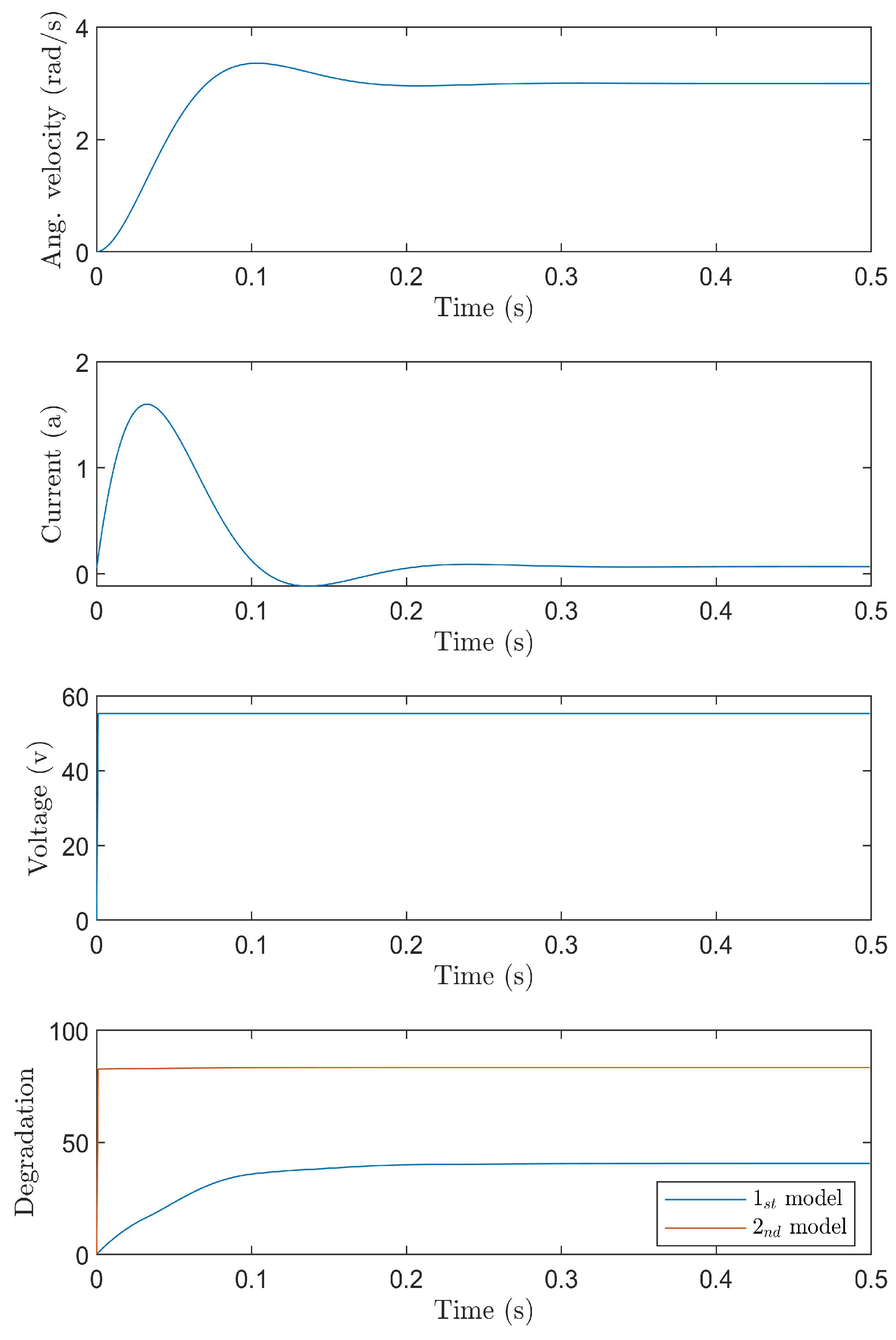
The response of the LQR when subjected to a step input of magnitude three, with the accompanying degradation that it imposed on the system, is depicted in
Figure 2. Choosing a step size of three, rather than one or two, enhanced the clarity when comparing the actions of the controller. This increased clarity came from the fact that a step size of three resulted in a more significant degradation of the system than step sizes of one or two. As a result, it became simpler to observe and assess the performance of the control method. Therefore, unless specified otherwise, the step response will be referred to as “step size of three”.
The degradation curve in
Figure 2 shows the effect of different system states or inputs on the degradation. The curves depict the parameter
described in Equations (32d) and (32e). The results show that the first degradation model was highly sensitive to variations in the system states, current, and angular velocity, as compared to the second degradation model, which was more influenced by the system input, that is, the voltage. Furthermore, the second degradation model exhibited significantly greater degradation of the system than the first degradation model.
In the next step, the degradation models mentioned in (32) were applied to (31), and data were recorded from the degrading machine.
These data were then used to calculate
and
, using (8) and (14). In the next step, the linear–quadratic degradation control feedback mentioned in (
16) was implemented for both degradation models mentioned in (31). Following the development of the LQDR controller, the production sequences for products 1, 2, and 3 were subjected to simulation, using a machine model that degraded over time, which was controlled by the LQDR algorithm. This simulation process continued until the occurrence of a failure, defined by the criteria outlined in Equations (
34) or (
35). The outcomes of these run-to-failure simulations, conducted for both the LQR and the LQDR controllers, are analyzed and compared in the subsequent sections.
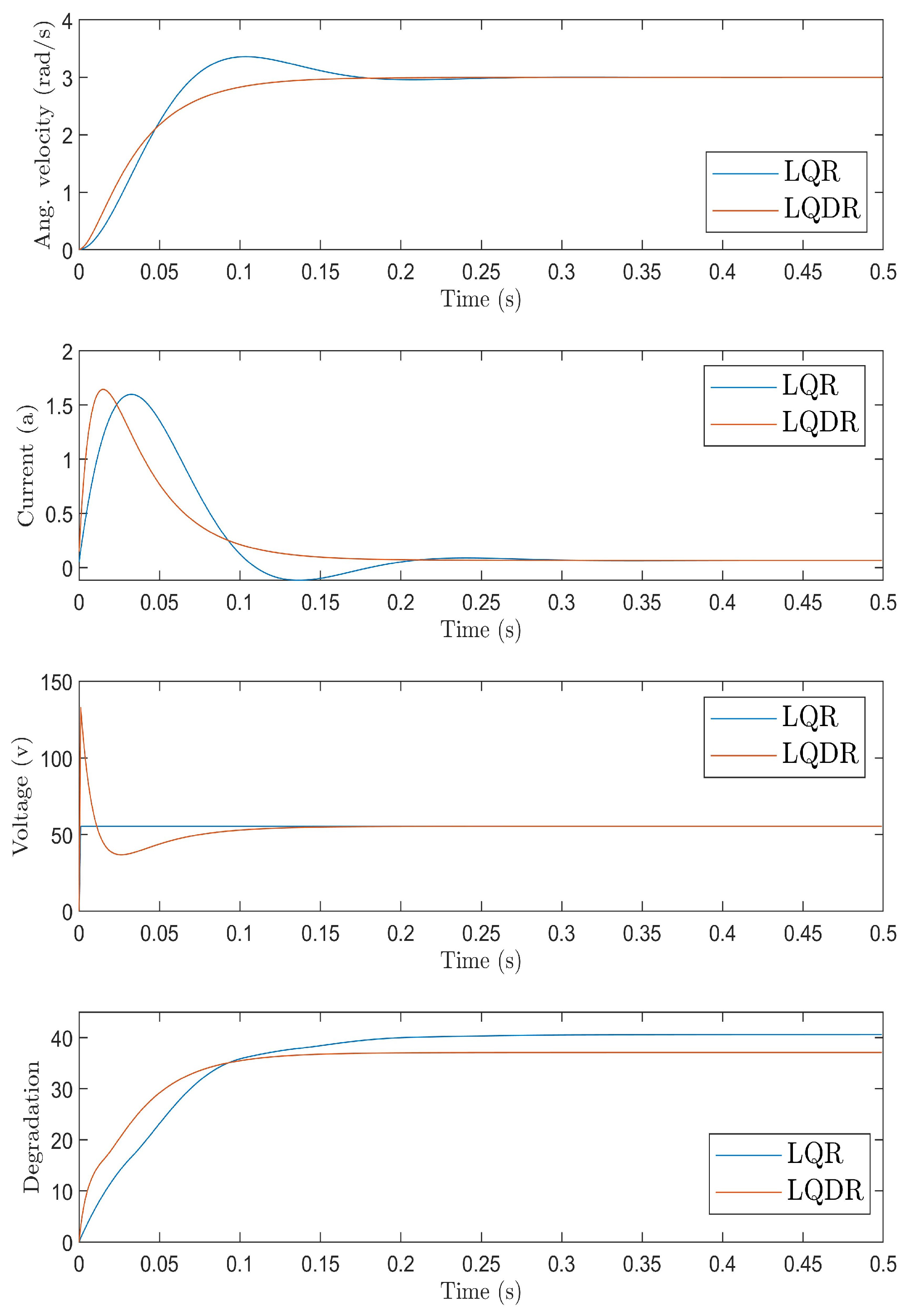
4.1. Controlling the First Degradation Model
Figure 3 displays the comparative responses of the LQR and the LQDR to the first degradation model. All the simulations in this section were conducted with fixed values of
equal to 1 and
equal to 2. In the case of the LQDR simulations, the value of
was held constant at
.
The difference between the control strategies is evident in the top three plots of
Figure 3. As anticipated, penalizing the controller for system degradation led to an increase in input usage, as changes in the input voltage resulted in a lower degradation rate than variations in the angular velocity and current. Consequently, the controller swiftly injected more voltage at the outset, even though this action may have initially exacerbated the machine’s degradation. Nonetheless, this course of action ultimately decreased the cumulative change in the system states over time, leading to a reduction in system degradation in the long term. This outcome can be seen in the bottom plot of
Figure 3, which displays the degradation (
from (32d)) experienced by both control strategies. It is apparent that the LQDR imposed less degradation on the system. This can be corroborated by
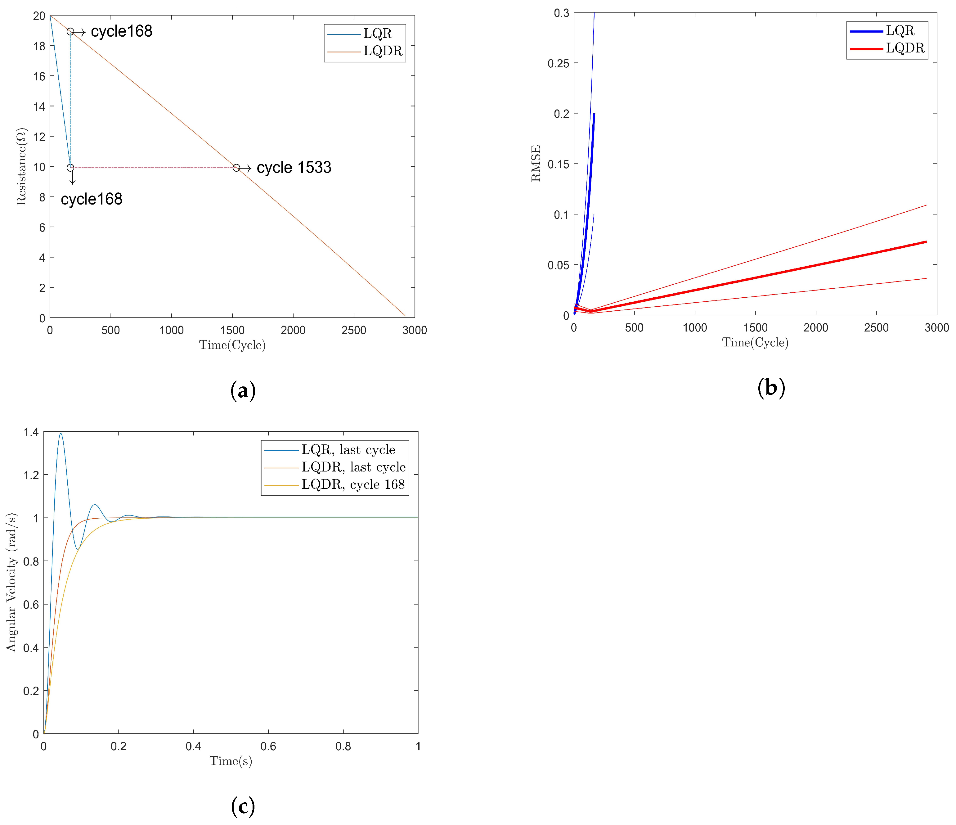
Figure 4a, which shows the degradation of the motor resistance over time using the LQR and the LQDR.
Figure 4a provides a visual representation of how the motor resistance deteriorated when controlled by both the LQR and the LQDR controllers. The simulation process for the machine, emphasizing its degradation, was carried out until it hit a failure threshold as defined in either (
34) or (
35). The findings from these simulations reveal a significant difference in durability between the two control strategies. Specifically, the LQR controller led to the machine reaching its failure point after merely 327 cycles. In contrast, the LQDR controller demonstrated a considerable improvement in longevity, enabling the machine to continue operating up to the 1521st cycle before succumbing to the failure criteria.
It is evident that the LQDR effectively protected the motor resistance from degradation.
Figure 4a illustrates that after 327 cycles the motor resistance lost only a fraction of its nominal value (less than
) while employing the LQDR. In contrast, when employing the LQR, the motor resistance lost half of its nominal value over the same number of cycles. Furthermore, the data demonstrate that the LQDR-controlled motor lost the same amount of resistance that the LQR-controlled motor lost during 327 cycles but took 890 cycles to do so. Additionally, the LQDR effectively controlled the motor until the resistance reached the lowest permissible value, as outlined in (
35) (i.e., 0.15 ohms). Conversely, the LQR lost control even when the motor resistance was still half of its nominal value. The evidence of this failure is demonstrated in
Figure 4b.
The RMSE of the output was analyzed for both the LQR and the LQDR and is presented in
Figure 4b. As mentioned, three desired outputs were considered for simulation. Each curve in
Figure 4b represents the RMSE of the output for desired outputs of 1, 2, and 3, respectively, for both the LQR and the LQDR. The lower lines on the graphs indicate the output RMSE for a desired output of 1; the thick middle lines represent the RMSE of the outputs for a desired output of 2, and the top lines indicate the RMSE of the desired outputs equal to 3.
It can be seen that motor-resistance degradation affected the output error of the LQR exponentially compared to the LQDR, which increased linearly. After 327 cycles, the RMSE of the output for the LQR exceeded the threshold. Specifically, the lower blue line, representing the output RMSE for a desired output of 1, surpassed the failure threshold of 0.1, as defined in (
34). However, at the same number of cycles, the RMSE for the output of the LQDR was considerably lower, which coincided with the reduction of the degradation in the motor resistance. Finally, it should be noted that unlike the LQR, which lost control after 327 cycles, the LQDR continued to operate until the maximum possible time when the resistance of the motor dropped below 0.15 ohms and the simulation stopped.
Figure 4c shows the unit step responses of the LQR and the LQDR at their final cycles prior to failure. By comparing the last operational cycle of both controllers, the impact of degradation on their responses can be discerned. Notably, the LQR controller demonstrated significantly lower resistance to internal parameter changes resulting from degradation than the LQDR. Specifically, the stability of the LQR was lost after 327 cycles, whereas the LQDR maintained stability even after 1521 cycles. To further illustrate this point, the response of the LQDR at cycle 327, during which the LQR failed, is plotted, highlighting the stable and accurate nature of the LQDR response. Based on the findings presented in this section, it can be concluded that the LQDR rather than the LQR provides better control quality in the face of changing system parameters due to degradation. Moreover, the LQDR’s ability to control machine degradation offers several distinct advantages.
4.2. Controlling the Second Degradation Model
For this section, the same methodology used in the previous section was employed to design a controller for a system undergoing degradation according to a second degradation model. As previously noted, the second model demonstrated that changes in voltage have a considerably greater impact on system degradation compared to the first model, as illustrated in the bottom plot of
Figure 2. Consequently, compensating for this degradation should result in a substantial increase in system lifetime.
Figure 5 shows the step response of the LQDR designed for the system degrading according to the second degradation model. Notably, optimizations in (8) and (14) effectively accounted for the impact of the system states and input on degradation, as demonstrated in the third plot of
Figure 5, where the rate of change in the input voltage in the LQDR has decreased compared to the LQR. This was due to the recognition of voltage changes as the parameter with the most significant effect on system degradation. As shown in the bottom plot of
Figure 5, degradation in the system significantly decreased in the LQDR compared to the LQR.
Figure 6a displays the degradation of motor resistance as affected by the second degradation model. The graphs depict how many cycles the LQR and the LQDR controllers were able to manage the machine before reaching a failure threshold, as outlined in (
34) or (
35). It is observed that the system experiencing the second degradation model had a comparatively shorter lifespan than the system subjected to the first degradation model, which was expected according to the degradation curves. Nonetheless, compensation for more severe degradation would further enhance the system’s lifespan. This phenomenon is evident in
Figure 6a,b, where the implementation of the LQDR enabled the system to operate for 2913 cycles by decreasing the motor resistance degradation and maintaining the output error below an acceptable threshold.
Figure 6c depicts the unit step responses of the LQR and the LQDR for their respective final operating cycles. Additionally, for comparative purposes, the response of the LQDR during cycle 168, the cycle in which the LQR failed, is also presented. Notably, it is evident that the LQDR for the second degradation model, similar to its performance in the first degradation model, effectively managed the variations in the nominal system parameters resulting from degradation while simultaneously mitigating degradation within the system.
Two points need to be addressed here regarding degradation control using the proposed method. First, it has been previously noted that two degradation models were developed to induce the controller to act in two opposed manners. Specifically, in the first degradation model, the increased voltage over shorter periods of time resulted in decreased degradation, while the opposite was true of the second model, where lower input voltage over longer periods of time reduced degradation. As a result, the same controller architecture with the optimal feedback introduced in (
16) and utilizing the same penalty matrix exhibited two entirely distinct modes of operation based on the working conditions or the unique degradation model of the system, which was derived through empirical analysis of historical data from the same system.
Second, the present study revealed that the LQDR exhibited two distinct features when compared to the conventional LQR. First, the LQDR demonstrated enhanced robustness against variations in system parameters, resulting in better control quality. This observation was supported by comparing the output error curves and unit step response curves before and after the degradation. Second, the LQDR mitigated motor-resistance degradation without explicit knowledge of the underlying degradation dynamics. This property is especially advantageous in systems with many states, where the physical analysis and modeling of the error may not be practically feasible while maintaining a high level of system reliability.
4.3. Validation Using SACM
Figure 7 provides additional insight into the control policy of the LQDR compared to the LQR. The plots displayed in
Figure 7 serve as an illustration of how the degradation controller operates in response to the unique degradation of the system.
The procedure for generating the SACM was explained previously. The graph comprises two components: first, an underlying image that displays the cost (
) introduced in (
37), and second, the state transition of the motor during the step response. The underlying image shows the total cost, which is the summation of three terms of (
37) for every feasible state–action combination quantized with a precision of 0.1 over the entire operational interval. A combination of states must be employed to accommodate all state combinations in a single y-axis, implying that the distance between states in SACM does not represent the actual distance in the real world. Additionally, lines between the circles are drawn to indicate the sequence of states through which the system passes, and the cost underlying the lines is not considered. Only the cost of the system states (the color underlying the circles) is regarded as the cost of the system’s actions.
Figure 7a,b show the step responses of the LQR and the LQDR plotted on the normalized SACM, which only includes the cost of the output error and input:
It can be seen that the reason for the behavior of the LQDR, especially in the system with the first degradation model shown in
Figure 7a, is not clear.
On the other hand,
Figure 7c,d show the same responses, this time plotted on top of the cost function that includes the degradation term,
As can be seen in
Figure 7c, the LQR response, represented by the blue curve, did not incorporate the degradation cost pattern into its behavior. In contrast, the LQDR response, depicted by the red curve, initially entered a high-cost region before swiftly transitioning to a prolonged period of low-cost operation, resulting in a greater proportion of time spent in a very low-cost region compared to the LQR response. Ultimately, the duration of time spent in the very low-cost region by the system will compensate for the duration of time spent in the high-cost region. This can also be seen in the bottom graph of
Figure 3.
The operation is more clear in
Figure 7d. It can be seen that the underlying cost map is different from the first model, due to the difference in the degradation models. Moreover, the elimination of costs is more transparent when comparing the results depicted in
Figure 7b. Note that the LQDR exhibited an improved awareness of the degradation cost included in the cost function and tried to remain in the low-cost region for as long as possible. Consequently, the level of degradation in the system diminished, leading to an increase in the system lifespan compared to the LQR.
5. Discussion
The summarized results from this section are presented in
Table 1. Notably, the overall enhancement of system reliability is closely tied to the penalty matrices, and the findings discussed here are grounded in the specific penalty matrices used.
Applying the LQDR led to observable improvements in system reliability across all criteria (control quality, RMSE, and MTTF). By reducing the degradation inflicted on the system, the LQDR effectively extended the system’s lifespan. Additionally, there was a significant reduction in the degradation rate in both instances examined.
The primary objective of the proposed approach is to control the system based on the empirical identification of degradation models. The empirical estimation of degradation cost has been demonstrated to offer significant advantages. Not only does it reduce the expenses associated with physically modeling the degradation, but it also produces outcomes that are physically interpretable and can be employed to control degradation.
The second aspect to be taken into account when designing this controller is the trade-off between control quality and degradation control. The addition of a new criterion to the optimization process will inevitably impact the final response. Therefore, the degree of degradation control must be calibrated based on the limits of the system error, or input can be increased. For instance, to assess the control quality of the system, a comparison of step functions between
Figure 4c and
Figure 6c can be made. Depending on the system type, such as drones or autonomous cars, it may be acceptable to trade off settling time for longer motor life. However, such trade-offs may not be acceptable for rolling mills where the output quality is critical. Thus, this compromise is very system-dependent and should be studied in detail before using the degradation control.
Another advantage of the proposed method is that not only the SoH but also the cost of other desired parameters, such as spare-parts prices, delivery delay, electricity bill, etc., can be calculated and included in the system control policy. Although the controller response considering all of these costs might not be acceptable, the availability of such information can facilitate the enhancement of designs towards more sustainable production or optimization of production and maintenance planning.
Finally, it is worth noting that the main limitation of this approach lies in the reliance on degradation control quality, on the unsmoothness of the degradation model, and on the available data processing capacity. This constraint arises due to the necessity of adopting a linear structure for
f, as mentioned in (
13), in order to achieve a closed-form infinite horizon feedback. In situations where the actual degradation model exhibits unsmooth and nonlinear characteristics, this assumption adversely impacts the quality of degradation control. Nevertheless, the accessibility of closed-form infinite horizon feedback offers the opportunity to compute multiple linear feedback for distinct operational intervals by treating the degradation model as piecewise linear. Thus, while this computation of diverse feedback mitigates the issue of nonlinearity, it introduces additional complexity to the system and demands a higher data-processing capacity.
The next phase of this research will focus on extending its application to other control strategies, such as finite-horizon control, which allows for the inclusion of greater nonlinearity in the system model. Additionally, integrating the SAC and degradation control mechanisms with PID control will be advantageous, given the widespread use of PID controllers in the industry.
6. Conclusions
This study introduces an innovative approach for managing degradation, thereby significantly enhancing system availability by controlling the reliability through controlling the degradation. A profound awareness of the implications of decisions and actions is instilled in the controller through the development of the control mechanism. An optimization technique that relies on historical data, rather than a specific system structure or degradation model, is employed, leading to the successful implementation of the empirical estimation of the SAC. This approach allows for the optimization of control actions aimed at managing degradation, with the costs of actions being directly incorporated into the feedback loop. The simulations clearly show that taking the costs of decisions into account, especially in terms of the SoH, significantly enhances the system’s availability, which is proportional to production reliability.
The foundation of the method lies in its unique independence from predefined system structures or degradation models, focusing instead on the empirical insights drawn from historical performance data. This independence allows for a flexible and adaptable approach to degradation control, capable of accommodating a wide variety of system types and operational conditions. Cost considerations are integrated into every aspect of the control strategy, ensuring that decisions are made with a comprehensive understanding of their potential impact on system health and longevity. The applicability across different contexts and the precision of degradation estimation and control are significantly improved by the empirical basis of the approach.
Finally, the results highlight the significant benefits of a cost-aware controller, which effectively extends the system’s lifespan through strategic degradation management. The simulations showed that a cost-aware controller could reduce the degradation rate from 0.03 to 0.01 in the first model and from 0.06 to 0.007 in the second. Moreover, this improved control over the degrading system significantly increased the motor’s operational life by about 5 times for the first degradation model and 17 times for the second model, respectively.
This advancement in control strategy represents a pivotal shift towards more sustainable and efficient system management, promising considerable benefits in terms of maintenance costs, system reliability, and overall performance. Looking ahead, the implications of this research open new horizons for exploring degradation control strategies that are both dynamic and predictive, paving the way for future innovations in system maintenance and reliability engineering.


