Reconstruction of Random Structures Based on Generative Adversarial Networks: Statistical Variability of Mechanical and Morphological Properties

Abstract

Generative adversarial neural networks with a variational autoencoder (VAE-GANs) are actively used in the field of materials design. The synthesis of random structures with nonrepeated geometry and predetermined mechanical properties is important for solving various practical problems. Geometric parameters of such artificially generated random structures can vary within certain limits compared to the training dataset, causing unpredicted fluctuations in their resulting mechanical response. This study investigates the statistical variability of mechanical and morphological characteristics of random 3D models reconstructed from 2D images using a VAE-GAN neural network. A combined multitool method employing different mathematical and statistical instruments for comparison of the reconstructed models with their corresponding originals is proposed. It includes the analysis of statistical distributions of elastic properties, morphometric parameters, and stress values. The neural network was trained on two datasets, containing models created based on Gaussian random fields. Statistical fluctuations of the mechanical and morphological parameters of the reconstructed models are analyzed. The deviation of the effective elastic modulus of the reconstructed models from that of the original ones was less than 5.7% on average. The difference between the median values of ligament thickness and distance between ligaments ranged from 3.6 to 6.5% and 2.6 to 5.2%, respectively. The median value of the surface area of the reconstructed geometries was 4.6–8.1% higher compared to the original models. It is thus shown that mechanical properties of the NN-generated structures retain the statistical variability of the corresponding originals, while the variability of the morphology is highly affected by the training set and does not depend on the configuration of the input 2D image.

1. Introduction

Methods for engineering the internal topology of materials and structures in order to achieve desired effective mechanical properties are actively developed [1,2,3,4,5,6]. In particular, the reconstruction of 3D microstructures based on limited input data plays an important role in materials design [7,8,9]. Artificial neural networks (NNs), which generate images resembling those in a training dataset, can be used to solve this problem and facilitate the design of new materials.

A variational autoencoder (VAE) was among the first attempts to synthesize 2D images with neural networks [10]. It consists of the encoder, which transforms an image into a latent vector, and the decoder, which maps this vector back onto the image. VAE was later combined with generative adversarial networks (GANs), which comprise a generator that synthesizes realistic images, and a discriminator that learns to distinguish between real images and fake ones created by the generator [11]. Currently, this idea is extensively developed and has attracted a great deal of attention from researchers in various fields [6,12,13,14].

Practical applications of such NNs include problems of establishing process–structure–property (PSP) relations. For instance, the generation of structures based on machine learning is a promising direction for addressing various biomedical challenges. For instance, the adjustment of geometric and mechanical characteristics of objects is one of the main tasks of personalized tissue engineering. X-ray or tomographic images of healthy tissue adjacent to the area to be replaced can serve as input data for such NNs. It is essential for the implant to have similar mechanical behavior and morphological structure to those of the original tissue [15,16,17].

Other reported successful applications of GANs were related to the reconstruction of heterogeneous materials [18,19,20], lattice structures [3,21], porous media [22,23,24], metamaterials [25,26,27], and architecture with extreme properties [6,28].

The quality of generated microstructures is usually evaluated by in-process quantitative measuring, for instance, by means of correlation functions and other morphological descriptors [8,29]. However, less attention is given to qualitative or statistical tools for direct comparison of the reconstructed models with their original counterparts. Geometric parameters of the generated models can vary within a certain range, affecting the resulting mechanical characteristics [30]. So, Zhu et al. [31] examined the task of shape reconstruction of 3D objects from a single 2D image using the so-called TL-embedding Network and 3D-VAE-GAN methods. The authors noted that despite its advantages, this approach could lead to object–shape distortion. To evaluate the effectiveness of VAE-GAN generation, Zhang [23] considered both isotropic and anisotropic porous stochastic media. A combination of these models resulted in more stable training and increased generation capability. Mosser [32] showed that GAN application for the reconstruction of stochastic porous media had the ability to match their key characteristics, such as two-point statistical measures, pore morphology, and directional single-phase permeability. However, the lack of information on porosity may affect the consistency of mechanical properties in the reconstructed models.

Currently, GAN’s technical difficulties, such as oversimplified models, requirements for oversized datasets, and inefficient convergence, can affect the quality of the generated structures [7]. Hence, it is important to suggest and apply a set of quantitative mathematical tools to capture differences between both mechanical and geometrical characteristics of the generated and original structures.

This study offers an approach for the investigation of the effectiveness of the reconstruction of 3D models from 2D slices based on a VAE-GAN NN by matching the mechanical characteristics and morphometric parameters of the generated and original structures using statistical analysis tools. The research question addressed by this study is whether the NN allows us to achieve the same variability of geometrical and mechanical parameters for the artificially reconstructed models as those of the original ones. A case study of the reconstruction of two-phase, open-cell, bicontinuous, random media is considered. Artificially generated structures based on Gaussian random fields were used as input data for the NN training. The task of the reconstruction of a 3D microstructure from a 2D slice is solved using the 2D-to-3D VAE-GAN, introduced in [33], which allows the creation of geometrically similar random structures. The reference set of 3D models, cross-sections of which were used as 2D input slices, was compared with the generated ones. An effective elastic modulus, a set of various morphometric parameters, as well as statistical distributions of maximum principal stresses obtained under a quasistatic tension load, were compared for the studied models employing statistical analysis tools.

The paper is structured as follows. Section 2.1 presents the methodology for creation of 3D bicontinuous random structures, which were used for training of the NN. Section 2.2 describes the architecture and working principle of the NN. Section 2.3 provides the formulation of the mechanical problem for numerical assessment of the mechanical properties and response of the original and generated models under a quasi-static tension load. Section 2.4 introduces morphometric characteristics for a quantitative description of the morphological composition and geometrical parameters of the original and generated geometric models. Section 3 presents the comparison of mechanical and morphometric parameters obtained for the models generated by the NN with the parameters of the reference models. A discussion of the results is provided in Section 4. Section 5 presents the conclusions.

2. Models and Methods

The methodology of this study includes the following steps illustrated in Figure 1: (i) creation of 3D models using a generator based on Gaussian random fields; (ii) configuration and training of the NN; (iii) creation of a set of reference 3D models and their cross-sections (2D slices) for the input data; (iv) reconstruction of 3D models from 2D slices; (v) validation of the generated structures by comparing the mechanical and morphological characteristics of the generated structures with the original ones.

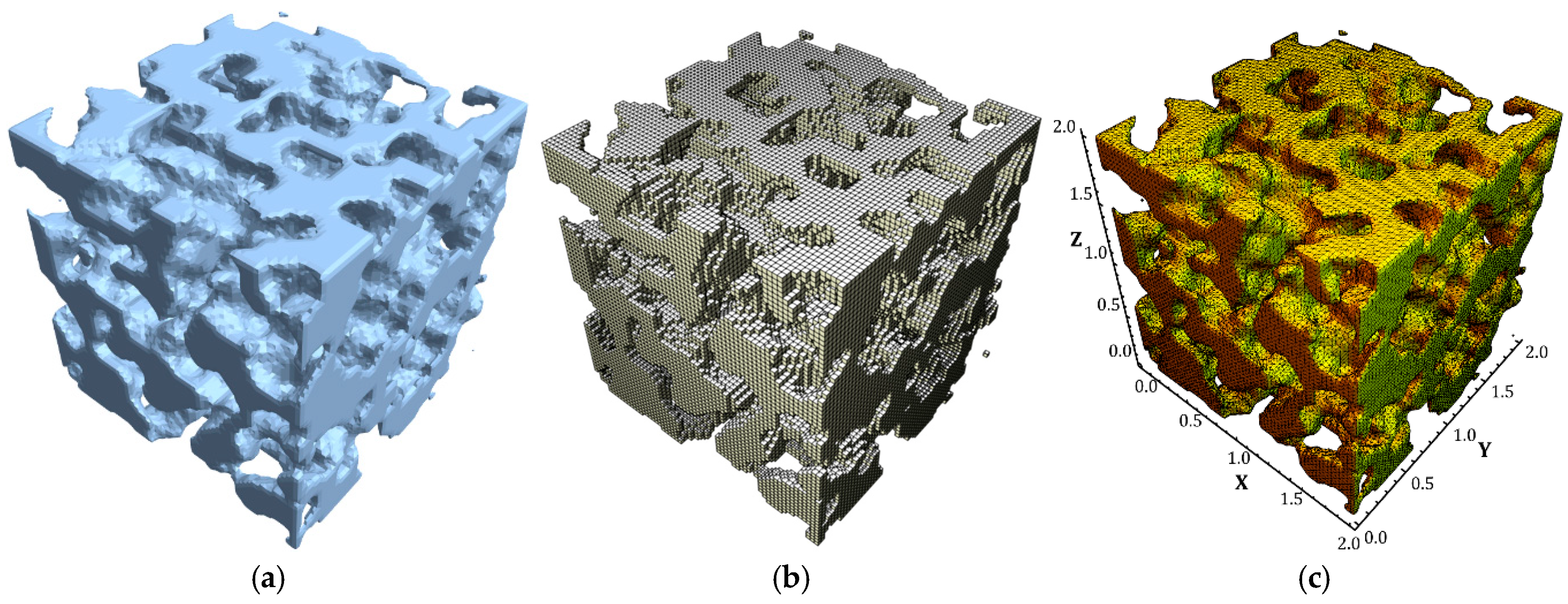
2.1. Synthesis of Random Open-Cell Bicontinuous Geometry

Open-cell, random, two-phase, bicontinuous models were used as a sample set for the NN training. Methods based on analytical determination of the interfacial surface were used to generate the geometry of such models [34]. Thus, random topology can be defined using the Gaussian random field, which contains the sum of waves with random parameters:

$$f\left(x\right)={\displaystyle \frac{1}{\sqrt{n}}}{{\displaystyle \sum }}_{i=1}^n{c}_i\cos \left({\displaystyle \frac{20}{L}}{k}_{i}x+{\phi }_i\right),$$

(1)

where $x$ is the position of the radius vector; $L$ is the representative volume size; n is the number of wave harmonics; $c_i=\sqrt{2}$ is the wave amplitude; and $k_i$ and ${\phi }_i$ are random variables.

A 3D two-phase structure is then created in two stages: (i) generating a random field in a 3D space and (ii) dividing all points of the generated field into two phases according to the level-set condition: a point belongs to the first phase if $f\left(x\right)<\xi$, and to the second phase if $f\left(x\right)\ge \xi$, where parameter $\xi$ affects the volume fraction of each phase. In this work, parameters $n=20$ and $\xi =0$ were used [34]. This algorithm creates structures with similar morphological characteristics, such as volume fraction, polydispersity, and the degree of structural order.

Equation (1) includes the random variables $k_i$ and ${\phi }_i$, whose distribution parameters affect the resulting geometry. The first set of models was created with a normal distribution of ki and φi with a mean of 0 and a variance of 1 (Type 1). The second set was created with a uniform distribution of $k_i$ and ${\phi }_i$ in the [0; 2$\pi$] interval (Type 2). The dimensions of the models considered were 2 mm × 2 mm × 2 mm. The volume fraction of the second phase (according to Equation (1)) was in the range of 0.44–0.53 for the Type 1 models (Table 1) and in the range of 0.43–0.53 for the Type 2 models (Table 2).

The original models of Type 1 and 2 are further denoted as R1 and R2, respectively.

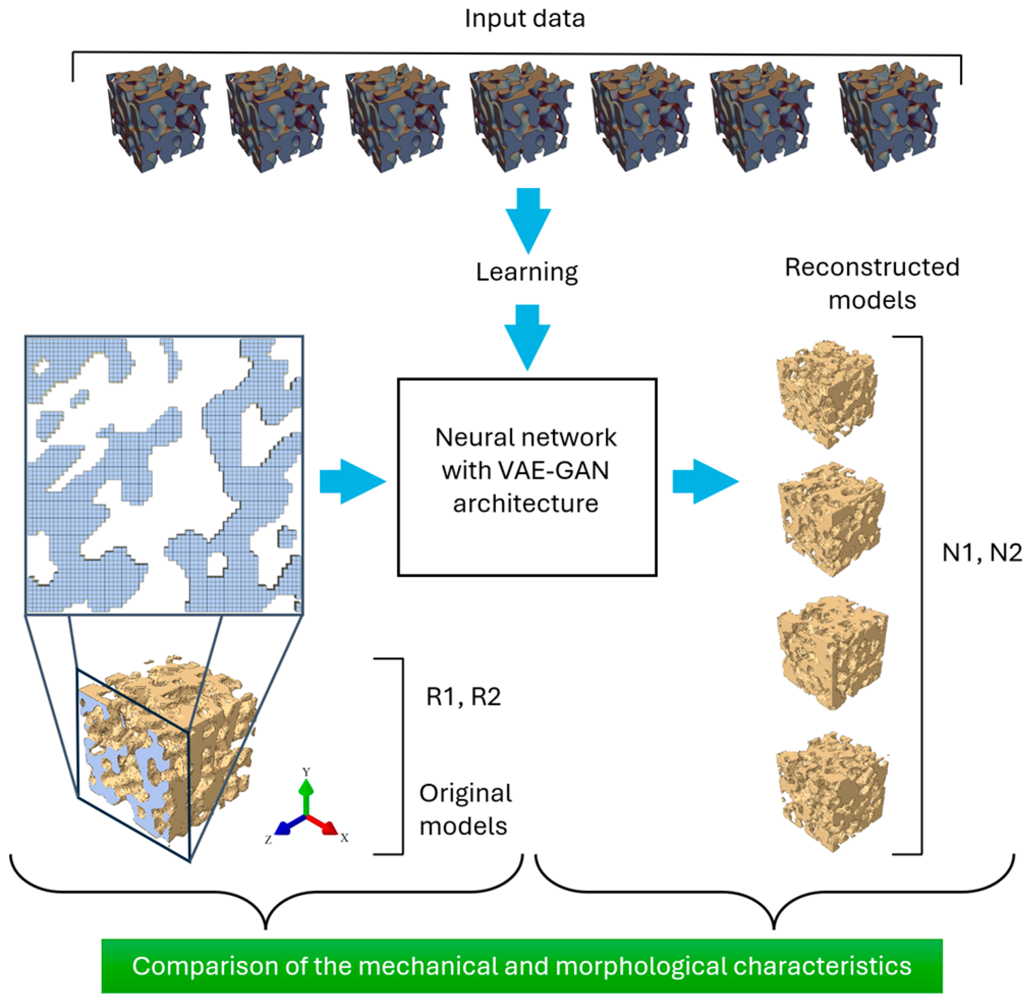
2.2. NN for 3D Reconstruction

The reconstruction problem was solved by utilizing the classical understanding of VAE-GAN [35] and rearranging it for the 2D-to-3D case [33]. Such a network includes three components: an encoder, a generator, and a discriminator. The encoder takes a 2D cross-section as an input and encodes it into a vector belonging to a latent space. Its goal is to explore the space of input images in order to produce an output of reduced dimensionality that contains information about their structure and characteristics. The generator’s task is to map the encoded vector of the properties of 2D slices onto 3D material microstructures. The training occurs in the form of a competitive game, where the generator learns to reconstruct realistic microstructures and “fool” the discriminator, while the discriminator learns to distinguish reconstructed microstructures from the original ones. The discriminator regularizes the encoder and the generator by learning the similarity metric between structures at the lth layer of the network.

For NN training, two sets containing 400 models of Types 1 and 2 were created using the method described in Section 2.1. The sample size for training in these case studies was chosen based on the complexity of the dataset as well as on the target performance metrics. The training data were a set of structures formalized as $m\times n\times n\times n\times c$, where $m=400$ is the number of models, $n=64$ is model resolution in voxels, $c=1$ denotes the number of channels. The encoder input had a form of $m\times n\times n\times c$. The encoder consisted of a series of 2D convolutional layers and had two outputs: the first was an expectation tensor $\mu$ and the second was a logarithm dispersion tensor $\log \left({\sigma }^2\right)$. They were used to create a latent $m\times l$ representation, with $l=64$:

$$z=\exp \left(\log \left({\sigma }^2\right)\right)\cdot N\left(0,I\right)+\mu ,$$

(2)

where $N\left(0,I\right)$ is the standard normal distribution.

To control the quality-criteria reconstruction, the two-point correlation function (2PCF) and the linear path function (LPF) were used [36,37,38]. The architecture of the generator and the discriminator, as well as details of training and testing of such NN, are described in [33].

2.3. Mechanical Characterization

For analysis of the mechanical response of the studied structures, the first phase was assumed to have linear-elastic isotropic behavior, modeled by polylactide (PLA) with the following properties: Young’s modulus of 2620 MPa and Poisson’s ratio of 0.36. The second phase was pores. All geometries were discretized into finite-element (FE) models with a two-step procedure (Figure 2). The first step involved the creation of a voxel FE model; at the second step, this model was transformed into a mesh of tetrahedral elements using the Dual Marching Cubes algorithm [39]. The maximum element size was 0.03 mm.

A mechanical response of the original and reconstructed models subjected to a tensile load was numerically analyzed in SIMULIA Abaqus. Boundary conditions included the rigidly fixed bottom face, while uniaxial tension with a force of 500 N was applied to the top face.

The effective elastic modulus for the axis, coinciding with the loading direction $z$, was determined as follows:

$$E_z={\displaystyle \frac{{\sigma }_z}{{\epsilon }_z}}={\displaystyle \frac{F·l}{S·\Delta l}},$$

(3)

where $F$ is the applied load; $S$ is the nominal area of the face of the model; $l$ is the length of the edge; $\Delta l$ is the elongation due to the applied load.

Stresses in finite elements can be considered as a realization of a random variable following some statistical distributions. Hence, taking the value of the stress field in each element as well as the element’s volume, the reverse problem of restoration of these distributions can be solved. The stress state of the whole model can be expressed then in the form of histograms, with its bars indicating the probability of finding the stress value in an element within a range corresponding to the bar. These histograms allow us to estimate the relative part of the finite elements in which the stresses (or stress invariants) exceed certain limits. For instance, if the samples are subjected to tensile loading and the brittle behavior of the material is assumed, particular attention should be paid to maximum principal stress (MPS). The critical stress value can be used as a threshold for distributions of probability density, which indicates the relative number of elements that fail under a given tensile load.

2.4. Morphological Characterization

Tools of the morphometric analysis were applied to evaluate the internal morphological composition of 3D random structures. Such tools are commonly used for the analysis of porous materials and applied, in particular, in the biomedical field for the analysis of bone-tissue parameters [40,41,42]. The thickness of structural elements (Tb.Th), the distance between them (Tb.Sp), and the area of the internal surface (Tb.BS) were considered. Tb.Th, at some point inside a two-phase structure, is defined as the diameter of the largest sphere that contains that point and can be entirely enclosed within the solid phase of the structure [43]. Accordingly, Tb.Sp is measured using such a sphere placed in the porous phase of the structure. To calculate Tb.BS, a surface area of the 2D boundary mesh needs to be computed. These characteristics for the studied geometrical models were calculated using the ImageJ image analysis program with the BoneJ plugin.

3. Results

3.1. 3D Model Reconstruction

Based on the input data (R1 or R2), two instances of the NN, presented in Section 2.2, were trained.

For each input 2D slice, such NNs can generate an infinite number of random 3D structures. To make conclusions about the effectiveness of the NN, it is important to assess the statistical distributions of mechanical and morphological parameters of the generated models. For this purpose, twenty 2D slices in the form of binary cross-sections with dimensions of 64 × 64 pixels were fed into the designed NNs. To prevent the NN from generating models from the training set, these input slices were taken from the different sets of R1 and R2 porous 3D models, which were not used for the NN training. The geometric models created by the NN that were trained on R1 and R2 datasets are referred to below as N1 and N2 models, respectively.

Twenty new 3D models were generated using both NNs for each of the twenty input 2D slices. Thus, based on the NN used, two sets of generated models, corresponding to the training sets with normal (N1) and uniform (N2) distributions of random parameters in Equation (1), were analyzed, forming an array of $20\times 20\times 2$ newly generated models in total. According to the method described in Section 2.2, the size of the reconstructed models was 64³ voxels. The method is schematically illustrated in Figure 1: a single face of the original R1 geometric model in the form of a pixelized image was fed as an input to the NN, which, being trained on the R1 dataset, reconstructed several N1 geometric models. The time for a single reconstruction of an RVE using GPU NVIDIA RTX A5000 was 0.053 s.

The specific feature of the proposed NN is that a 2D slice, provided as input, does not appear as any cross-section in a generated model.

The ranges of volume fraction of the porous phase in the reconstructed N1 and N2 geometric models, based on 20 input images, are presented in

Table 1. Volume fraction (VF) of porous phase in R1 models, whose faces were used to create their reconstructed analogues N1.

Slice No.	VF of R1 Model	VF Range in Twenty N1 Models	Slice No.	VF of R1 Model	VF Range in Twenty N1 Models
1	0.494	0.46–0.52	11	0.443	0.481–0.546
2	0.506	0.438–0.522	12	0.498	0.455–0.538
3	0.509	0.478–0.539	13	0.499	0.495–0.545
4	0.514	0.425–0.524	14	0.495	0.453–0.535
5	0.511	0.449–0.536	15	0.503	0.474–0.52
6	0.463	0.489–0.545	16	0.511	0.47–0.535
7	0.494	0.479–0.53	17	0.511	0.48–0.53
8	0.53	0.474–0.532	18	0.443	0.465–0.539
9	0.506	0.453–0.529	19	0.525	0.471–0.541
10	0.525	0.475–0.514	20	0.48	0.45–0.546

and

Table 2. Volume fraction of porous phase in R2 models, whose faces were used to create their reconstructed analogues N2.

Slice No.	VF of R2 Model	VF Range in Twenty N2 Models	Slice No.	VF of R2 Model	VF Range in Twenty N2 Models
1	0.5	0.486–0.526	11	0.509	0.487–0.561
2	0.514	0.47–0.52	12	0.496	0.479–0.52
3	0.51	0.45–0.529	13	0.509	0.461–0.506
4	0.495	0.465–0.558	14	0.499	0.479–0.527
5	0.502	0.479–0.547	15	0.504	0.471–0.536
6	0.526	0.479–0.54	16	0.505	0.453–0.547
7	0.5	0.475–0.54	17	0.51	0.485–0.538
8	0.534	0.459–0.53	18	0.508	0.476–0.54
9	0.481	0.461–0.51	19	0.428	0.467–0.536
10	0.508	0.465–0.52	20	0.508	0.474–0.531

and illustrated as box plots (Figure 3 and Figure 4, respectively). The horizontal line inside the plot represents the median of the dataset, while the points outside the box lie beyond the range equal to 1.5 times the interquartile range (IQR).

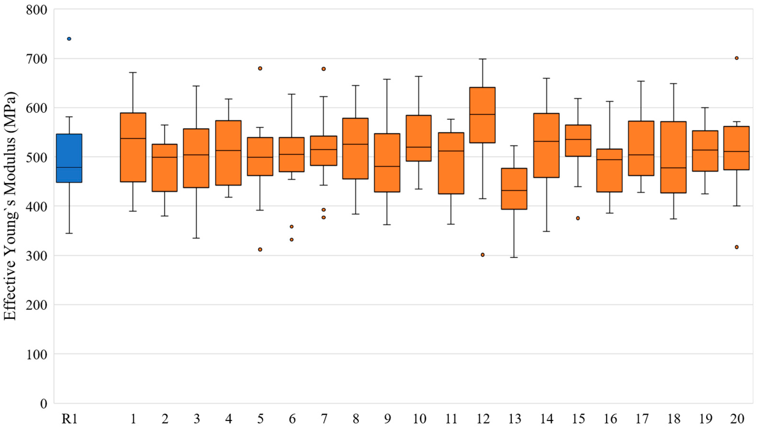
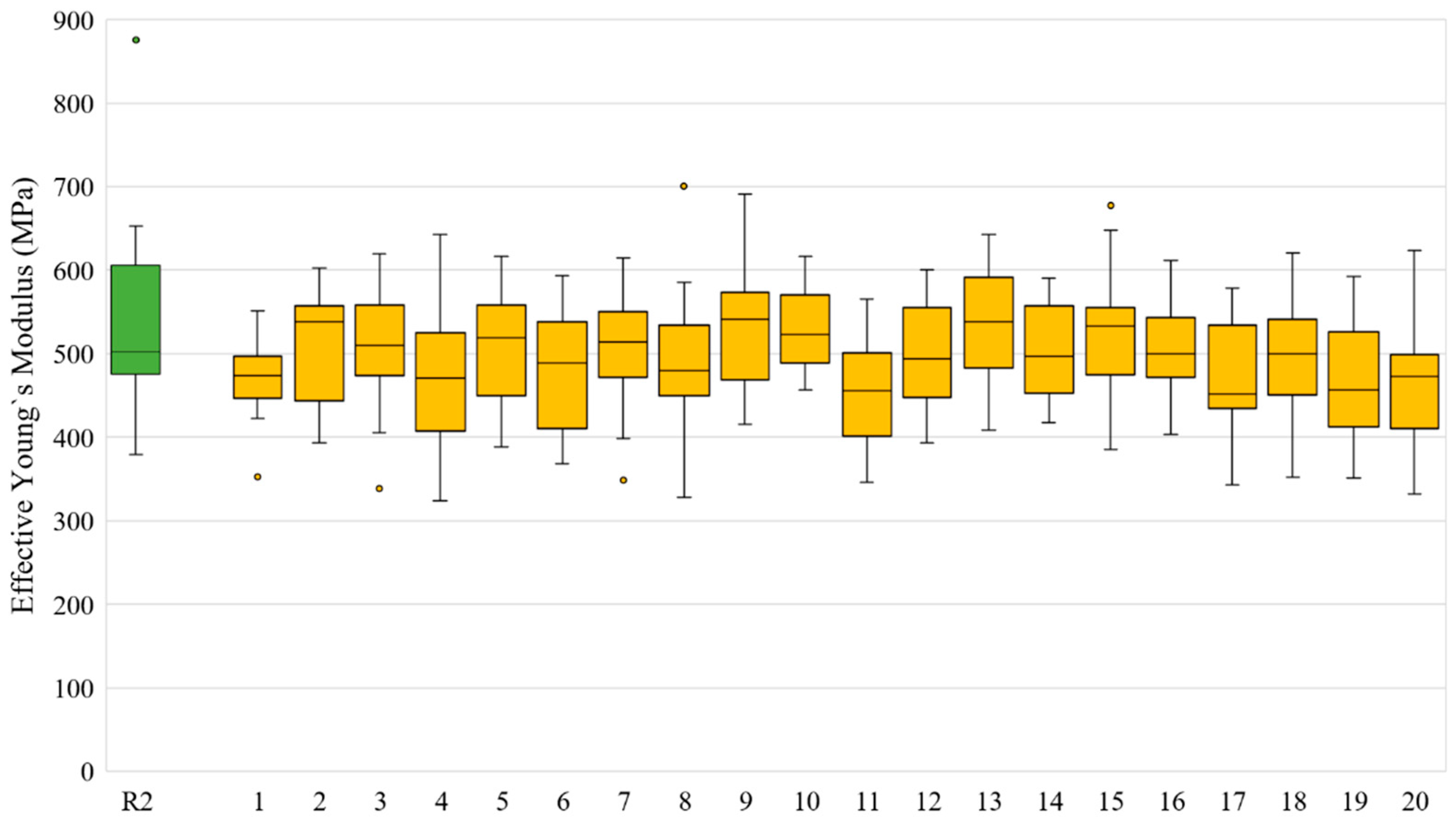
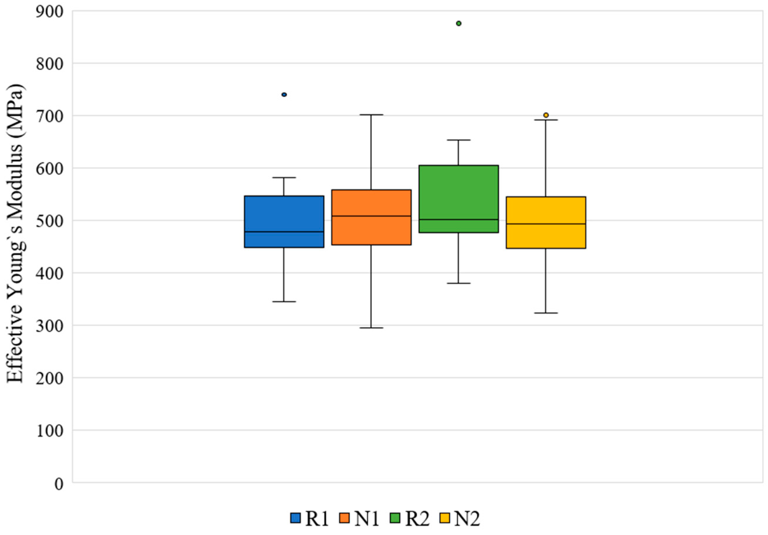
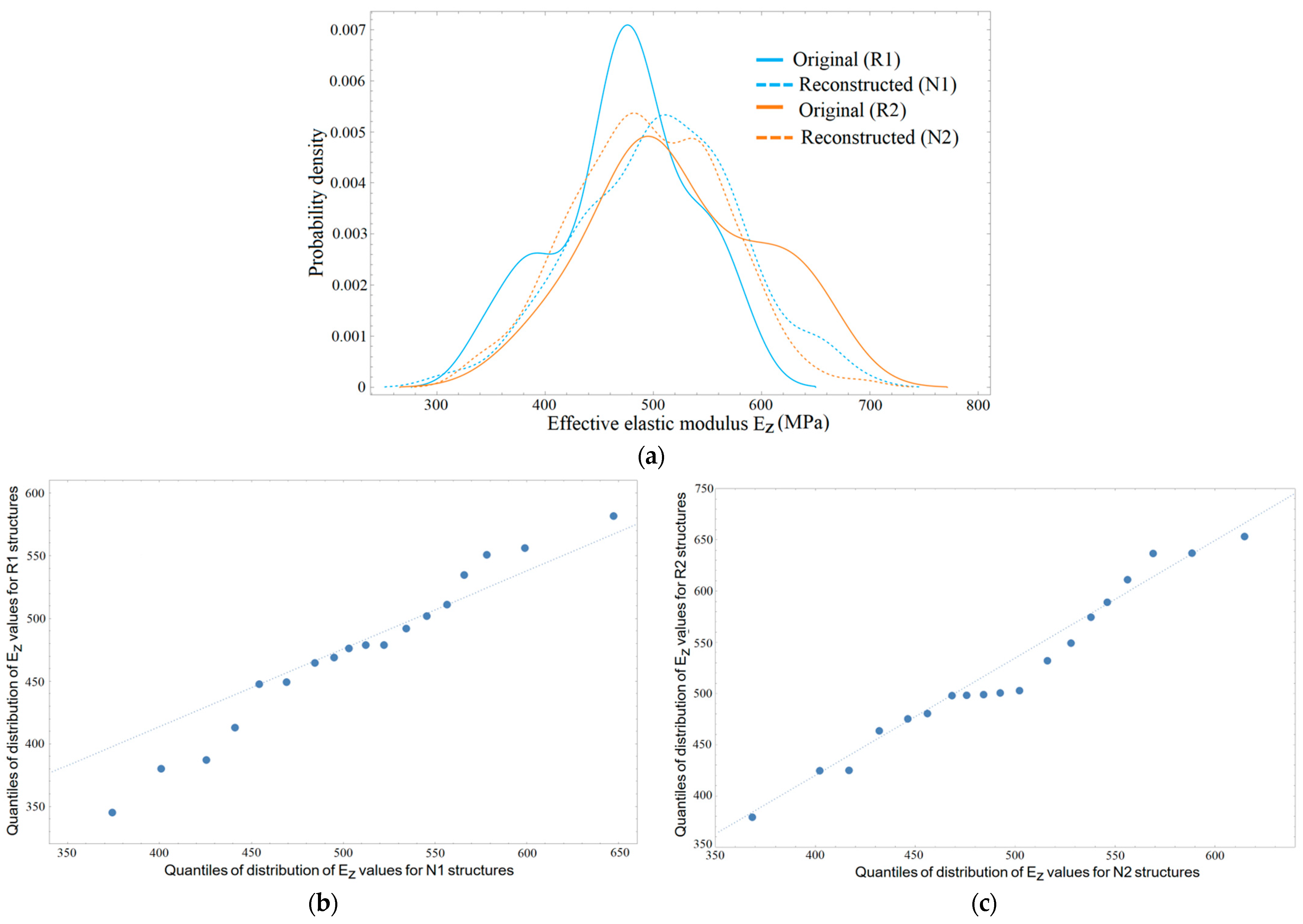
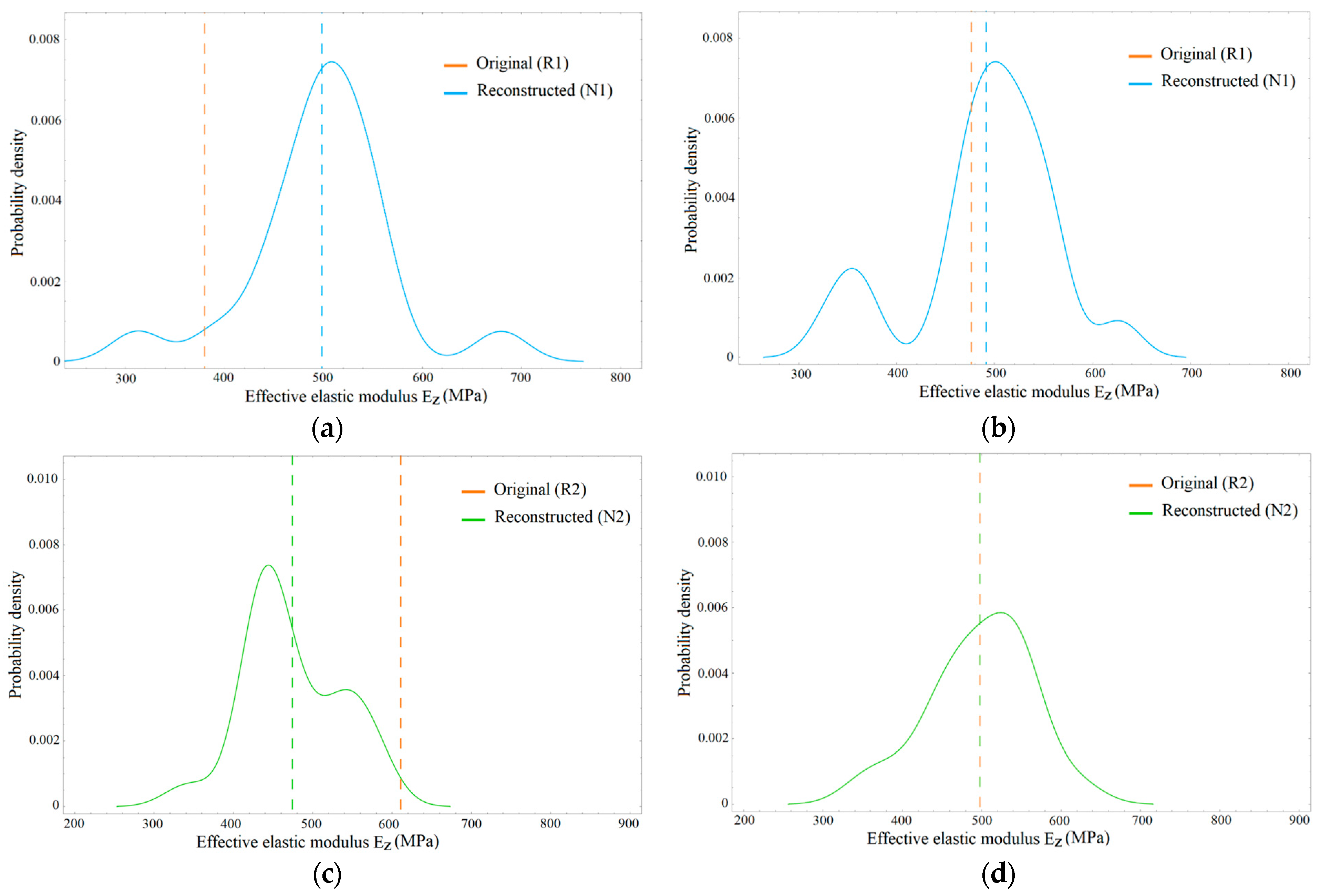
3.2. Distribution of Elastic Properties

Values of the effective Young’s modulus $E_z$ were calculated based on the results of numerical FE simulations of generated N1 and N2 models (800 in total) as well as for the corresponding original R1 and R2 models (40 in total). They are presented in

Table 3. Effective elastic moduli $E_z$ of original R1 models and the statistical properties for their N1 reconstructed analogs.

Slice No.	${\mathit{E}}_{\mathit{z}}$ for R1 Models (MPa)	$\mathbf{Median}\mathbf{Value}\mathbf{of}{\mathit{E}}_{\mathit{z}}$ for 20 Corresponding N1 Models (MPa)	$\mathbf{Trimmed}\mathbf{Mean}{\mathit{E}}_{\mathit{z}}$ for 20 Corresponding N1 Models (MPa)	$\mathbf{Winsorized}\mathbf{Mean}{\mathit{E}}_{\mathit{z}}$ for 20 Corresponding N1 Models (MPa)	Standard Deviation for 20 Corresponding N1 Models (MPa)
1	478.50	537.43	527.90	528.42	77.63
2	344.93	499.39	483.14	482.27	54.66
3	468.57	503.89	502.52	503.22	77.28
4	534.22	512.83	509.74	510.49	69.81
5	379.80	498.89	498.40	496.11	72.38
6	476.04	504.72	492.58	489.46	72.22
7	478.50	514.56	511.56	511.14	69.78
8	555.98	525.79	522.43	521.66	77.19
9	491.85	480.24	484.56	485.88	78.18
10	501.85	519.70	531.97	533.13	66.36
11	739.72	511.62	494.01	491.40	70.19
12	449.01	585.96	578.18	574.29	92.85
13	550.57	432.03	429.85	427.87	58.31
14	386.92	531.04	526.41	525.60	85.91
15	510.97	535.63	527.47	526.24	55.94
16	412.73	494.08	480.32	479.58	60.51
17	447.53	504.20	513.87	516.50	66.60
18	739.71	477.58	488.47	488.64	79.37
19	464.28	514.03	513.03	512.71	52.74
20	581.40	510.79	514.02	511.21	76.60
Average	532.81	535.43	527.81	524.24	117.86

and

Table 4. Effective elastic moduli $E_z$ of R2 models and median $E_z$ values for their reconstructed analogs N2.

Slice No.	${\mathit{E}}_{\mathit{z}}$ for R2 Models (MPa)	$\mathbf{Median}\mathbf{Value}\mathbf{of}{\mathit{E}}_{\mathit{z}}$ for 20 Corresponding N2 Models (MPa)	$\mathbf{Trimmed}\mathbf{Mean}{\mathit{E}}_{\mathit{z}}$ for 20 Corresponding N2 Models (MPa)	$\mathbf{Winsorized}\mathbf{Mean}{\mathit{E}}_{\mathit{z}}$ for 20 Corresponding N2 Models (MPa)	Standard Deviation for 20 Corresponding N2 Models (MPa)
1	636.42	473.70	472.02	472.60	44.31
2	379.01	537.96	510.56	509.71	67.67
3	652.94	509.55	512.63	512.26	70.51
4	500.36	470.38	472.57	473.63	78.17
5	474.85	518.48	504.32	504.48	66.95
6	424.79	488.62	476.54	476.88	73.71
7	636.73	513.74	506.85	505.62	66.83
8	463.30	480.01	482.89	482.93	79.75
9	589.12	540.67	527.99	529.48	73.18
10	497.85	523.00	524.97	524.85	49.46
11	424.18	455.25	449.39	448.56	61.16
12	549.15	493.57	498.13	498.15	60.58
13	502.68	538.19	533.11	532.47	68.05
14	531.89	496.76	500.67	499.99	55.01
15	498.59	533.04	522.16	522.11	78.55
16	480.08	500.03	504.31	503.31	52.58
17	610.82	451.57	475.69	478.28	60.39
18	497.93	500.07	499.19	496.79	64.78
19	875.21	456.66	460.50	459.69	65.88
20	574.36	472.18	459.28	458.75	73.65
Average	562.67	513.71	518.14	526.33	111.33

for models of Types 1 and 2, respectively. The results for the Type 1 original and reconstructed models are presented in Figure 5.

The median values for most of the N1 models were between 500 and 530 MPa, which aligns with its distribution for R1 models (with notable discrepancies for structures No. 12 and 13). The IQRs of all box plots are quite large: 60–145 MPa, comparable to that of the R1 models (99 MPa). The median of the effective modulus for R1 models was 479 MPa. The original R1 models had two outliers with elastic modulus values significantly higher than those for the others in the set (corresponding to 2D slices No. 11 and 18). However, that did not lead to any visible differences in the corresponding plots obtained for their N1 reconstructed analogues (see plots No. 11 and 18 in Figure 5). The reconstructed N1 models had a considerable number of outliers (nearly 3%), and some box plots had whiskers nearly as large as the IQR.

It can be concluded that deviation in the median effective properties of the reconstructed N1 models from their original R1 did not exceed 27%. The smallest deviation of 2.42% was observed for slice No. 9. The arithmetic means of deviations in the median effective elastic modulus of the reconstructed N1 models, considering all twenty R1 models, was 16.72%.

In addition to the median value, the trimmed (when outliers are disregarded) and winsorized (when a threshold is applied, after which the extreme values are replaced with the remaining extreme) means were also calculated. These averaging methods allow assessment of the influence of the outliers. Thus, the greatest impact on the median mean was exerted by the outliers in groups No. 2 and 11 of the reconstructed structures. The difference between the median and the trimmed mean for both reconstructed groups was 3.36%, and the difference between the median and the winsorized mean was 3.54% and 4.11% for groups No. 2 and 11, respectively. This indicates that excluded outliers had an insignificant effect on the median values.

Similarly, results for the effective elastic modulus $E_z$ for 400 N2 models for R2 models corresponding to each of the generating slices of 20 original R2 models were obtained. They are presented as box plots in Figure 6.

The median values of most of the N2 box plots were between 470 and 530 MPa, which is within the corresponding range of values for the original R2 models. However, there is a significant mismatch for the structures generated based on slice No. 11. The IQRs for all the boxes were quite large, from 80 to 113 MPa, but smaller than that for the R2 models’ distribution (130 MPa). The median value of the effective elastic modulus for the R2 models was 502 MPa. There was one outlier in the set of R2 models (No. 19), but it did not affect the corresponding plot for the set of N2 reconstructed models. The R2 models showed a large IQR and a similarly large lower whisker, indicating very high variability. In contrast, N2 models had fewer outliers (around 1%), but many of the box plots’ whiskers were comparable in size to the IQR.

Based on Figure 6 and Table 4, it can be concluded that the difference between the median values of the effective elastic modulus for N2 models and the corresponding R2 models also did not exceed 27% (excluding outliers). The minimum deviation (0.43%) in the median effective elastic modulus was observed for model No. 18. The average of these deviations, considering all 20 R2 models, was 17.61%.

The extreme values in groups No. 2 and 17 of the N2 models had the greatest impact on the median value. When the outliers were removed from the sample (trimmed mean), the mean values decreased by 5.37% and 5.07%, respectively. However, if the outliers were not removed but instead replaced with the smallest and largest values from the remaining data set (winsorized mean), the mean values decreased by 5.54% and 5.58%, respectively. As with Type 1 structures, the standard deviation was higher for the effective elastic modulus of the original structures compared to those of the reconstructed ones. The difference between these values was 66.76%, but when outliers were excluded from the R2 sample, it decreased to 18.60%. This demonstrates that the type 2 models had a larger distribution of the elastic modulus, which still was in an acceptable range.

The distributions of the effective elastic-modulus values for generated N1 and N2 models as well as for the corresponding original R1 and R2 models are compared in Figure 7.

The median values of the effective elastic modulus for the N1 and N2 models were 507 MPa and 492 MPa, respectively. The difference between the median effective elastic modulus values for the N1 models and their generating R1 models was 5.66%, whereas for the R2 and N2 models, it was 1.74%. The IQR and positions of the box plots for the R1 and N1 models were nearly identical, indicating that their distribution areas for the middle 50% of the data were similar. In contrast, it was not the case for the R2 and N2 models: despite the small difference in median values, the IQRs of these box plots differ significantly.

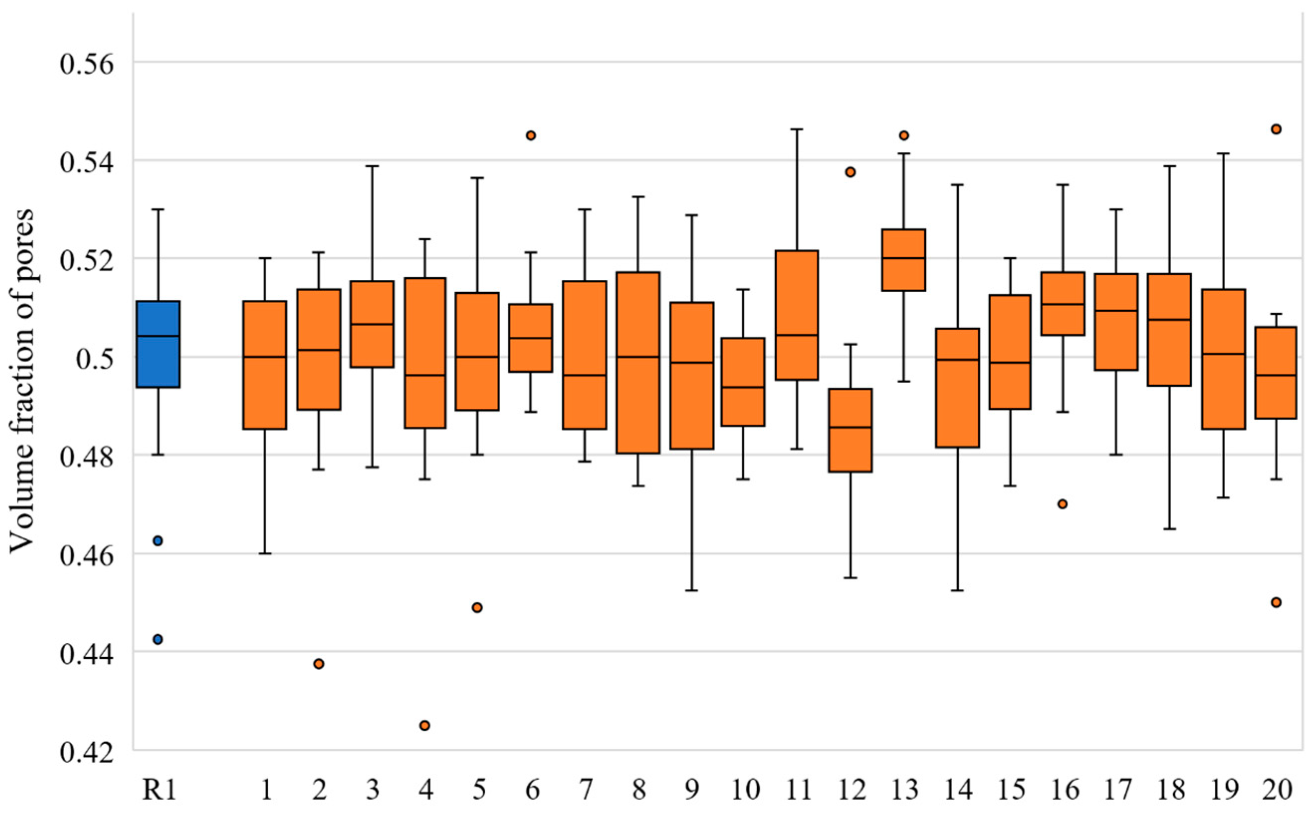
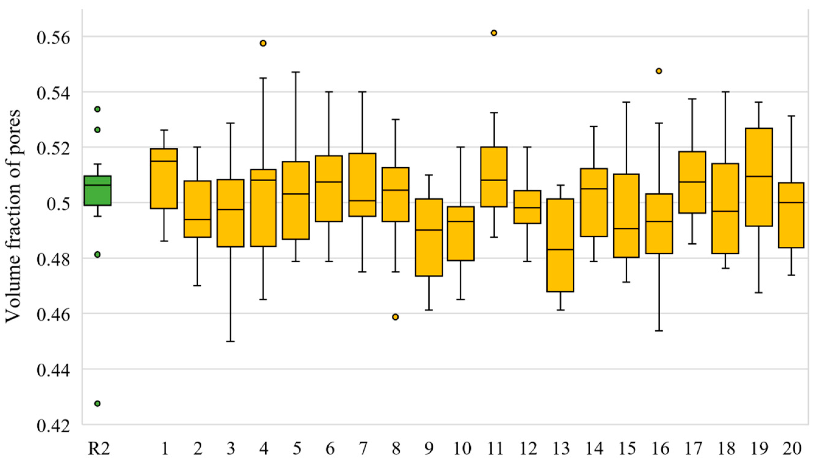
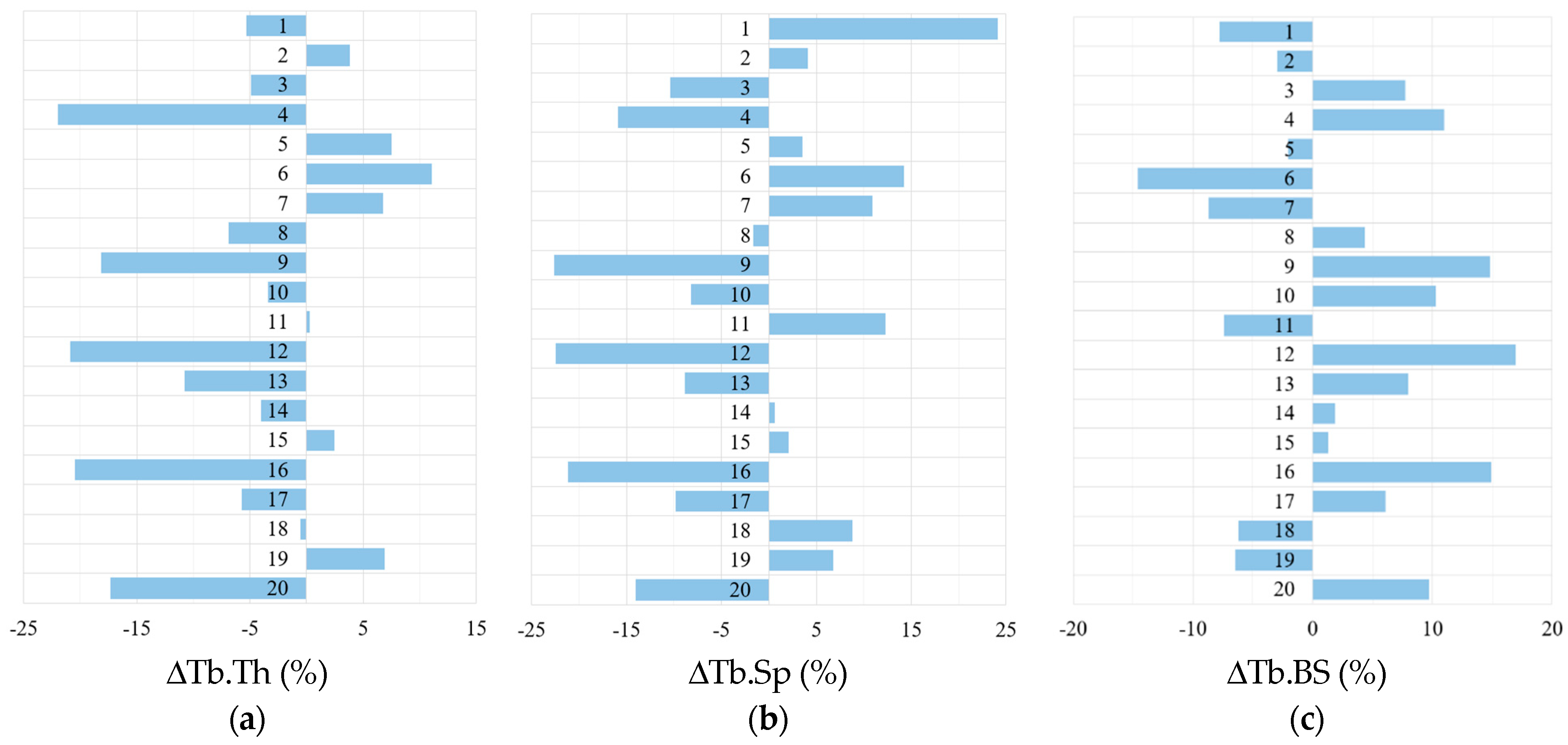
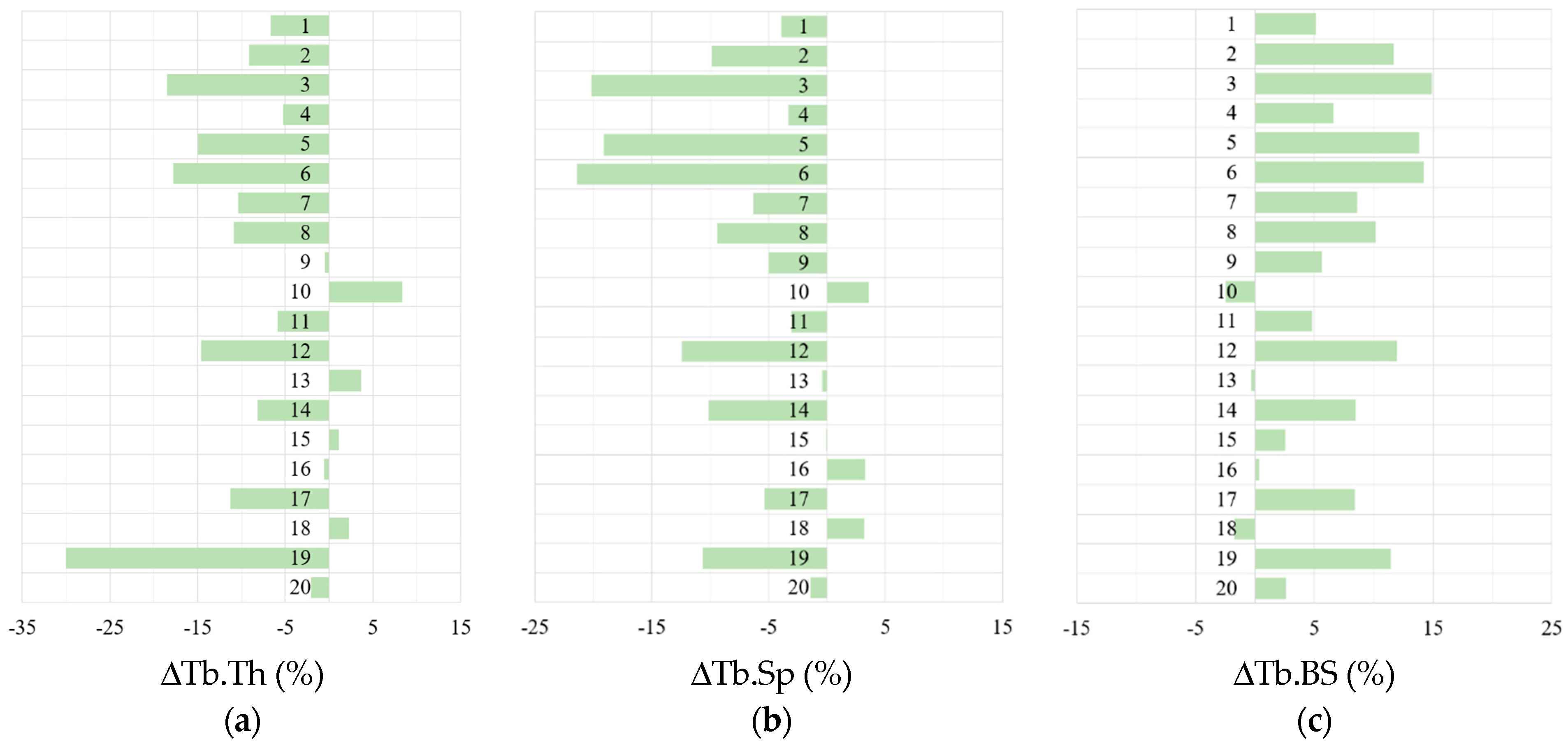
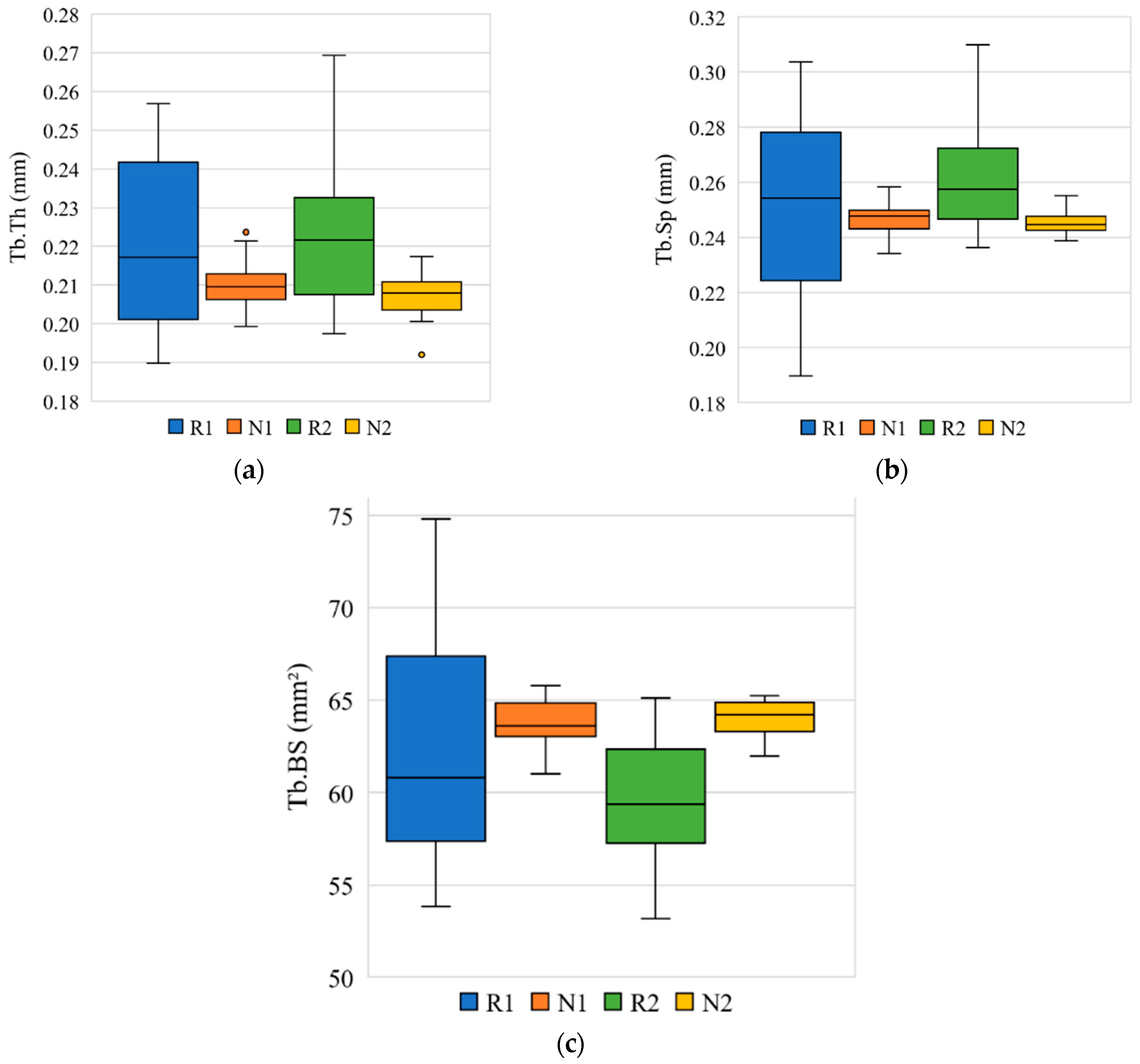
3.3. Morphometric Analysis

In each group of 20 reconstructed models, the morphometric analysis was performed only for the one with the effective elasticity modulus closest to that of their corresponding original model. Figure 8 presents the difference (in percentages) between the morphometric parameters, such as ligament thickness Tb.Th., the distance between ligaments Tb.Sp., and surface area Tb.BS, for the reconstructed N1 models in comparison with their closest R1 model.

The maximum difference between N1 and R1 models for the ligament thickness (Tb.Th.) was −21.99%, for the distance between ligaments (Tb.Sp.), it was 24.13%, and 16.98% for the surface area (Tb.BS). The maximum ligament thickness among the original R1 models corresponded to slice No. 9, while among the reconstructed models, it was in model No. 14. Models No. 9 and No. 14 (both R1 and N1) exhibited the largest distances between ligaments. The values of parameters corresponding to the N1 models showed a lower dispersion compared to the R1 models. For instance, the parameter Tb.BS for the N1 models was 64.32 ± 10.47 mm², while for the R1 models, it was 63.38 ± 2.39 mm².

The morphometric characteristics of the Type 2 models exhibited some noticeable patterns (Figure 9). In most cases, the values for Tb.Th. and Tb.Sp. obtained for the generated N2 models were lower than those for the corresponding original R2 models. However, most of the reconstructed models had a higher surface area. Hence, despite the matching effective elastic modulus, the geometric parameters of the reconstructed and original models were different: the difference between the morphometric values reached 30.1%. As in the previous case, R2 models exhibited a broader dispersion in values of the studied parameters. Thus, the Tb.BS parameter for the R2 models ranged from 53.17 mm² to 65.11 mm², while for the N2 models, it ranged from 61.97 mm² to 65.24 mm².

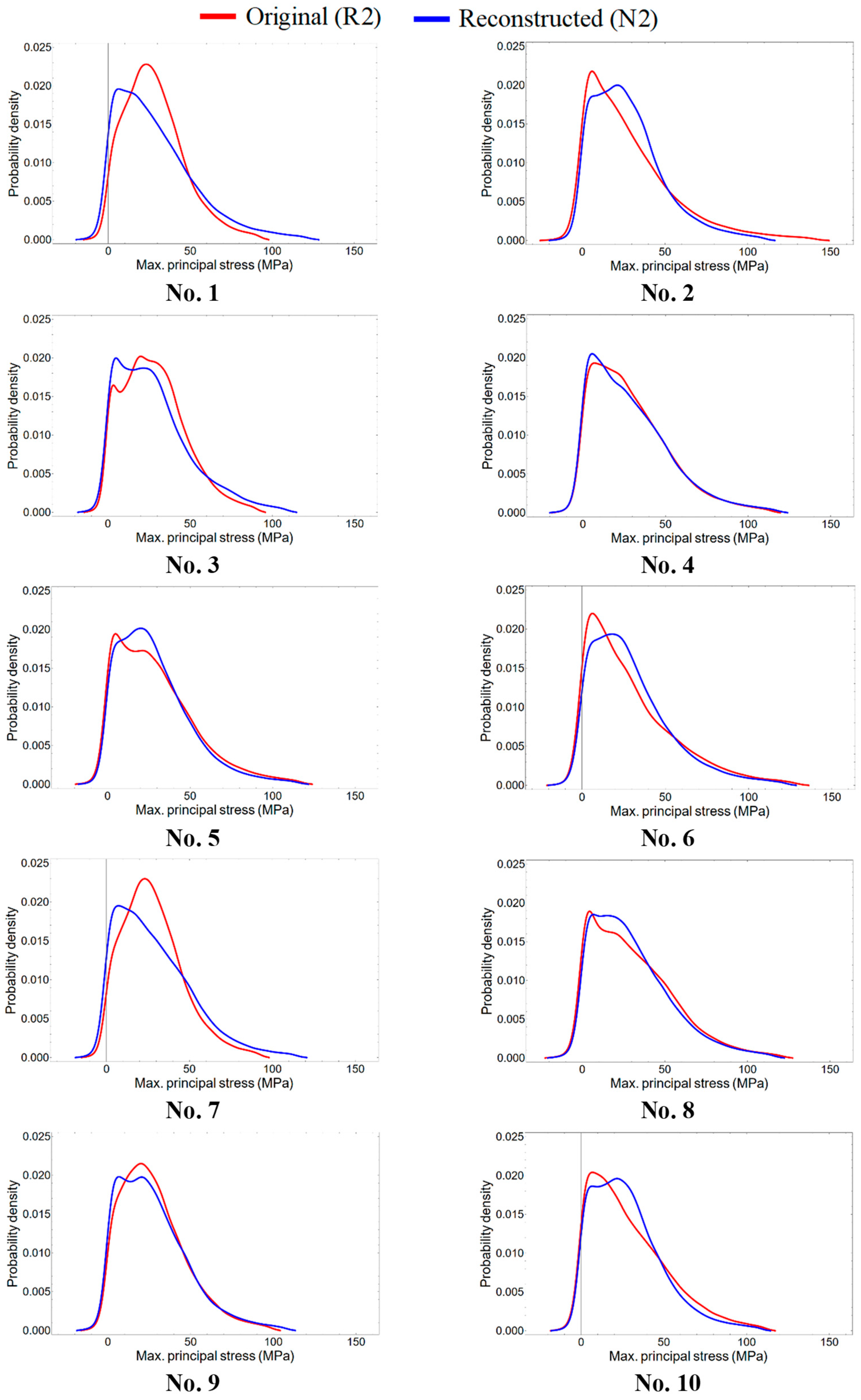
3.4. Stress Distributions

The probability density distributions of maximum principal stresses in the FE models as a result of a tensile load of 50 N are presented as smoothed histograms in Figure 10 and Figure 11 for the Type 1 and Type 2 models, respectively. Similar to the morphometric analysis, a single reconstructed model closest to the original model values of the effective elastic modulus was selected for each set for detailed examination.

The probability density distributions for all the examined structures were close to the skew-normal distribution. The stresses occurring in the models of both types were within the same range. The smoothed histograms for the original R1 and reconstructed N1 models were almost identical. Additionally, in most cases, the probability density plot of the maximum principal stresses was unimodal. There was no clear dependence of the obtained plots on the values of the effective modulus of elasticity or the morphometric characteristics. It can be observed that N2 models based on slices No. 1, No. 3, and No. 7 exhibited higher stress values compared to their originating R2 models. This means that the reconstructed models were able to replicate the stress-strain response of the original models within the framework of the elastic formulation.

4. Discussion

4.1. Effective Elastic Modulus

The deviation of the effective elastic modulus of the reconstructed models from that of the original ones did not exceed 27% when considering individual R-N pairs and was less than 5.7% on average for the entire sets of specimens. Outliers of the effective elastic modulus were 2% of the total of the two sets of specimens.

The probability density plots of the effective elastic modulus are presented as smoothed histograms (Figure 12a). Figure 12b,c displays quantile-quantile (Q-Q) plots of the distribution of effective Young’s modulus values for R1 and R2 structures (40 structures) against the quantiles of the distribution for N1 and N2 structures (800 structures), respectively. The y-coordinate at a point (x, y) on the graph corresponds to the quantile of the distribution of the elastic moduli of reconstructed structures, plotted against the same quantile (x-coordinate) of the distribution of corresponding values for the original structures. The resulting intersection of the quantiles is indicated by dots on the graphs. If the distributions match, the points lie on a bisector. It should be noted that the outliers discussed above were excluded from the set of values obtained for the original structures.

The probability density plots of the effective elastic modulus values for the Type 2 models were closer to each other than those corresponding to the Type 1 models. The shape of the plots resembles that of a normal distribution. The maximum probability density for the reconstructed N1 structures was 24.7% lower than that for the R1 structures. It was also noticeable that the reconstructed N1 models exhibited higher values of the effective Young’s modulus compared to the models from which they were reconstructed. As for the Type 2 models, the higher values are characteristic of the R2 models.

From the Q-Q plots (Figure 12b,c), it is evident that the points are not on the bisector, indicating that the distributions did not exactly match. Additionally, the plot has a wave-like shape, suggesting that one of the distributions is more distorted than the other. At the lower and upper ends of the range for the Type 1 models, the deviations were observed, while some points in the center are on, or rather close to, the straight line. This indicates that the central quartiles of these distributions correspond to each other. For the Type 2 models, the central quartiles were closer to the distribution of the reconstructed N2 models. It can be seen in Figure 12c that the extreme points (the minimum and maximum values of the effective elastic modulus) are nearly on the straight line, indicating a similar range of values for the R2 and N2 models.

Additionally, probability density plots of the effective Young’s modulus were constructed for each group of reconstructed structures. Figure 13 shows graphs corresponding to the original structures No. 5 and 6 of Type 1 and 17 and 18 of Type 2. The plots highlight the mean values of the effective elastic modulus for the reconstructed structures (blue and green lines), as well as the $E_z$ value for the original structure from which the reconstruction was performed (orange line).

In most cases, the values of the effective characteristics of the original structures were in the central quartiles of the distribution. The values corresponding to the effective elastic modulus of structures No. 11 of Type R1 and No. 1 and 19 of Type R2 fell outside the range of the distribution of these values obtained for the reconstructed structures. The mean values of the effective elastic modulus for structures No. 6, 9, and 15 of Type N1, as well as No. 18 of Type N2, almost coincided with the $E_z$ values of the corresponding original structures. Thus, it can be concluded that the average value of the elastic modulus of the reconstructed structures depends more on the effective properties of the training sample than on the structure from which it was created.

4.2. Correspondence of Internal Stress State

The probability density distributions of the maximum principal stresses, presented in Section 3.4, were compared using Pearson’s chi-squared test (see

Table 5. Probability of correspondence between the maximum principal stress distributions of original and reconstructed structures.

Type 1		Type 2
Slice No.	$\mathit{p}$	Slice No.	$\mathit{p}$
1	0.01	1	0.26
2	0	2	0.3
3	0.01	3	0.09
4	0.2	4	0
5	0.02	5	0.29
6	0.05	6	0.05
7	0	7	0.15
8	0.02	8	0.1
9	0	9	0.06
10	0.25	10	0.3
Average	0.056	Average	0.16

). By default, such test function returns a calculated probability $p$. A hypothesis (commonly called the null hypothesis) about the coincidence or inconsistency of the distributions under consideration should be made. In this study, the null hypothesis assumed that the stress distributions of the original and reconstructed structures were not the same. Therefore, the null hypothesis is rejected if $p<\alpha$, with the significance level $\alpha$ set at 0.05.

Most p-values obtained for structures of Type 1 were smaller than α, indicating that the hypothesis that the two distributions do not match should be rejected. Hence, there was a good similarity between the distributions of maximum principal stresses for the original and reconstructed structures of Type 1. However, Type 2 structures predominantly show p-values greater than the given significance level α. This indicates that the null hypothesis cannot be rejected, and maximum principal stress distributions demonstrate, in general, lesser similarity.

4.3. Morphometric Characteristics and Statistical Metrics

The diagrams presented in Figure 14 illustrate the obtained distributions for the investigated morphometric parameters.

The values and positions of the IQRs of the morphometric parameters for the original and reconstructed models did not coincide. The morphometric parameters obtained for the reconstructed models exhibited a smaller spread of values compared to those of the original models; this pattern was independent of the type of models. The median values of ligament thickness and the distance between ligaments for the original models were higher than those for the reconstructed models. The difference between the median values of ligament thickness and distance between ligaments for the reconstructed and original models ranged from 3.6 to 6.5% and 2.6 to 5.2%, respectively. The median value of the surface area for N1 structures was 4.6% higher, while for N2 structures, it was 8.1% higher compared to the original models.

In the example of the Type 1 models, it can be observed that even though the traditional metrics, such as measured cumulative distributions, lineal path, and two-point correlation functions were close to the original and reconstruction models (see Figure 15), the resulting distributions of the morphological values (which also reflect the internal geometry) were different (see Figure 14).

The investigation into the variability of morphometric characteristics revealed that the reconstructed models had noticeably limited ranges of these values compared to the original 3D models. This can be due to the fact that the 2D cross-sections, used as an input for the NNs, had limited information about morphological features compared to the 3D structure. Thus, the suggested NN reconstructs a 3D structure with morphometric characteristics similar to those of the models used for its training. More control can also be achieved by incorporating additional morphological metrics during the generation process, with established relations to the discussed main morphometric parameters.

4.4. Achievements, Limitations and Possible Extensions

Several methods can be used to assess the variability of geometrical parameters of models generated by VAE-GANs (see

Table 6. Mathematical tools and metrics used to quantify the variability of models generated by VAE-GAN.

Tool	Description	Function
Fréchet Inception Distance (FID) [44]	Measures the distance between the feature distributions of real and generated images	Quality and diversity of generated samples
Chamfer Distance (CD) [45]	Quantifies the similarity between sets by calculating the average distance from each point in one set to its nearest neighbor in the other set	3D shapes and their variability
Root Mean Square Error (RMSE) [45]	A standard metric for measuring the differences between predicted and actual values	Reconstruction accuracy and variability in generated 3D models
Latent Space Visualization Techniques [46]	Allow visualization of high-dimensional latent space representations in a lower dimensional form	How variations in latent variables affect generated outputs
Statistical analysis of geometrical quantities [47]	Analyses variance, standard deviation, and entropy of geometrical features of generated samples	Provides quantitative assessment of geometrical
Statistical analysis of mechanical and morphological properties (the present work)	Analyzes morphological characteristics, elastic properties, and stress distributions	Provides quantitative assessment of geometrical features as well as of mechanical response

). Common metrics like Fréchet Inception Distance (FID) or Chamfer Distance (CD) may not fully capture all the features of 3D structures, leading to potential misinterpretations of variability. Besides, in terms of reconstruction of materials, the mechanical response is as important as geometrical fidelity and needs to be estimated.

The combination of tools proposed in this work allows us to compare the variability of the mechanical response of the artificially generated structures in combination with the morphological characteristics.

The studied VAE-GAN NN with incorporated statistical descriptors as quality metrics demonstrated its effectiveness in generating a range of structures with similar mechanical properties, which, however, could not achieve the original statistical variability of the morphometrical characteristics. This can be resolved by introducing the proposed variability metrics directly into the VAE-GAN algorithm, which is the focus of future work.

In the considered case studies, the structures were subjected to a simple mechanical load scenario (tension), assuming that this is the predominant loading mode for the studied materials. In practical applications, the loading conditions could be different, which will affect the applied load in numerical models as well as the types of measured elastic properties and stress distributions. However, the general workflow of the approach will remain the same. Besides, if needed, the number of measured properties could be increased to assess the variability of generated structures in different cases. This can be useful for those VAE-GANs that are able to generate structures with anisotropic properties.

The introduced stress distributions can also be used as estimators of structural integrity by introducing a strength criterion, which can be used for calculating the volume fraction of failed elements as well as failure probability. This was not implemented in the present study, but such failure probability can serve as another metric in the extensions of the suggested approach.

In general, the proposed tools are intended to be used for any two-phase geometrical models with a voxel-based representation. The possible extension of the suggested methodology is related to the VAE-GANs that can reconstruct multicomponent materials consisting of more than a single solid phase. In this case, the suggested statistical tools should be updated accordingly. For instance, stress distributions can be compared in each phase of the material, and the scalar morphometric characteristics can be substituted with functionals depending on the local phase.

5. Conclusions

This paper investigated the effectiveness of the method for the reconstruction of 3D random models based on 2D slices using the VAE-GAN neural network by comparing statistical variation of mechanical and morphological characteristics for both the original and generated models.

The NN was trained with two datasets of models created based on the Gaussian random fields with normal and uniform distributions of random variables. Correspondence between the generated models and the original ones was assessed by comparing their mechanical and morphological characteristics, such as elastic modulus, morphometric parameters, and microscale stress distributions.

The mechanical properties of the generated structures were evaluated using numerical finite-element simulation of models under a tensile loading regime. The median values of the effective elastic properties for the generated models were within the range of those values for the original models. On average, in a set of 20 reconstructed models generated from a single cross-section, only a few models exhibited either very high or low elastic moduli. The analysis of the probability density distributions of maximum principal stresses under the tensile load in the original and reconstructed models generally showed a similar mechanical response. However, reconstructed models of Type 1 showed better correspondence to the originals than the Type 2 models. In a few cases, under the same loading conditions, stresses in the reconstructed models exceeded the maximum stresses observed in the original models.

The morphometric parameters of the investigated structures were also analyzed. The values of ligament thickness, distance between ligaments, and surface area for the reconstructed models with normally distributed parameters were close to the corresponding mean values obtained for the originals. However, despite matching the effective elastic modulus values between models with uniformly distributed parameters, their morphometric characteristics did not always statistically coincide. In particular, ligament thickness and distance between them for the reconstructed models were lower than those of the original structures. In both studied cases, the original structures exhibited a broader distribution of morphometric parameter values compared to the reconstructed models, although their traditional quality metrics, such as lineal path and two-point correlation functions, were close.

The practical application of the suggested approach is connected with the analysis of variations of the structures with specific properties generated from limited experimental data. The generative models allow for sophisticated analysis of material properties and relationships, facilitating the identification of patterns that can guide further research. This is particularly useful in the field of materials design, where understanding the microstructure is crucial for predicting material properties and establishing a connection between microstructural features and macroscopic properties.

References

1. Yuan, X.; Zhu, W.; Yang, Z.; He, N.; Chen, F.; Han, X.; Zhou, K. Recent Advances in 3D Printing of Smart Scaffolds for Bone Tissue Engineering and Regeneration. Adv. Mater. 2024, 36, e2403641. [Google Scholar] [CrossRef] [PubMed]
2. Brown, N.K.; Garland, A.P.; Fadel, G.M.; Li, G. Deep reinforcement learning for the rapid on-demand design of mechanical metamaterials with targeted nonlinear deformation responses. Eng. Appl. Artif. Intell. 2023, 126, 106998. [Google Scholar] [CrossRef]
3. Hsu, Y.C.; Yang, Z.; Buehler, M.J. Generative design, manufacturing, and molecular modeling of 3D architected materials based on natural language input. APL Mater. 2022, 10, 041107. [Google Scholar] [CrossRef]
4. Generale, A.P.; Robertson, A.E.; Kelly, C.; Kalidindi, S.R. Inverse stochastic microstructure design. Acta Mater. 2024, 271, 119877. [Google Scholar] [CrossRef]
5. Ng, W.L.; Goh, G.L.; Goh, G.D.; Sheuan, J.; Ten, J.; Yeong, W.Y. Progress and Opportunities for Machine Learning in Materials and Processes of Additive Manufacturing. Adv. Mater. 2024, 36, e2310006. [Google Scholar] [CrossRef]
6. Mao, Y.; He, Q.; Zhao, X. Designing complex architectured materials with generative adversarial networks. Sci. Adv. 2020, 6, eaaz4169. [Google Scholar] [CrossRef]
7. Zheng, Y.; Li, Z.; Song, Z. A generative machine learning model for the 3D reconstruction of material microstructure and performance evaluation. Comput. Methods Appl. Mech. Eng. 2024, 430, 117224. [Google Scholar] [CrossRef]
8. Lyu, X.; Ren, X. Microstructure reconstruction of 2D/3D random materials via diffusion-based deep generative models. Sci. Rep. 2024, 14, 5041. [Google Scholar] [CrossRef]
9. He, J.; Kushwaha, S.; Abueidda, D.; Jasiuk, I. Exploring the structure-property relations of thin-walled, 2D extruded lattices using neural networks. Comput. Struct. 2023, 277, 106940. [Google Scholar] [CrossRef]
10. Kingma, D.P.; Welling, M. Auto-Encoding Variational Bayes. arXiv 2013, arXiv:1312.6114. [Google Scholar]
11. Goodfellow, I.J.; Pouget-Abadie, J.; Mirza, M.; Xu, B.; Warde-Farley, D.; Ozair, S.; Courville, A.; Bengio, Y. Generative Adversarial Networks. Adv. Neural Inf. Process. Syst. 2014, 27, 2672–2680. [Google Scholar] [CrossRef]
12. Zeng, Q.; Zhao, Z.; Lei, H.; Wang, P. A deep learning approach for inverse design of gradient mechanical metamaterials. Int. J. Mech. Sci. 2023, 240, 107920. [Google Scholar] [CrossRef]
13. Challapalli, A.; Patel, D.; Li, G. Inverse machine learning framework for optimizing lightweight metamaterials. Mater. Des. 2021, 208, 109937. [Google Scholar] [CrossRef]
14. Jiao, P.; Alavi, A.H. Artificial intelligence-enabled smart mechanical metamaterials: Advent and future trends. Int. Mater. Rev. 2021, 66, 365–393. [Google Scholar] [CrossRef]
15. Oladapo, B.I.; Zahedi, S.A.; Ismail, S.O.; Olawade, D.B. Recent advances in biopolymeric composite materials: Future sustainability of bone-implant. Renew. Sustain. Energy Rev. 2021, 150, 111505. [Google Scholar] [CrossRef]
16. Fujita, A.; Goto, K.; Ueda, A.; Kuroda, Y.; Kawai, T.; Okuzu, Y.; Okuno, Y.; Matsuda, S. Measurement of the Acetabular Cup Orientation After Total Hip Arthroplasty Based on 3-Dimensional Reconstruction From a Single X-Ray Image Using Generative Adversarial Networks. J. Arthroplast. 2024, 40, 136–143. [Google Scholar] [CrossRef]
17. Wu, C.; Wan, B.; Entezari, A.; Fang, J.; Xu, Y.; Li, Q. Machine learning-based design for additive manufacturing in biomedical engineering. Int. J. Mech. Sci. 2024, 266, 108828. [Google Scholar] [CrossRef]
18. Yang, Z.; Yabansu, Y.C.; Al-Bahrani, R.; Liao, W.K.; Choudhary, A.N.; Kalidindi, S.R.; Agrawal, A. Deep learning approaches for mining structure-property linkages in high contrast composites from simulation datasets. Comput. Mater. Sci. 2018, 151, 278–287. [Google Scholar] [CrossRef]
19. Yang, Z.; Li, X.; Brinson, L.C.; Choudhary, A.N.; Chen, W.; Agrawal, A. Microstructural materials design via deep adversarial learning methodology. J. Mech. Des. Trans. ASME 2018, 140, 111416. [Google Scholar] [CrossRef]
20. Yang, Z.; Yabansu, Y.C.; Jha, D.; Liao, W.K.; Choudhary, A.N.; Kalidindi, S.R.; Agrawal, A. Establishing structure-property localization linkages for elastic deformation of three-dimensional high contrast composites using deep learning approaches. Acta Mater. 2019, 166, 335–345. [Google Scholar] [CrossRef]
21. Zhang, H.; Yang, L.; Li, C.; Wu, B.; Wang, W. ScaffoldGAN: Synthesis of Scaffold Materials based on Generative Adversarial Networks. CAD Comput. Aided Des. 2021, 138, 103041. [Google Scholar] [CrossRef]
22. Shams, R.; Masihi, M.; Boozarjomehry, R.B.; Blunt, M.J. A hybrid of statistical and conditional generative adversarial neural network approaches for reconstruction of 3D porous media (ST-CGAN). Adv. Water Resour. 2021, 158, 104064. [Google Scholar] [CrossRef]
23. Zhang, F.; Teng, Q.; Chen, H.; He, X.; Dong, X. Slice-to-voxel stochastic reconstructions on porous media with hybrid deep generative model. Comput. Mater. Sci. 2021, 186, 110018. [Google Scholar] [CrossRef]
24. Chiang, Y.H.; Tseng, B.Y.; Wang, J.P.; Chen, Y.W.; Tung, C.C.; Yu, C.H.; Chen, P.Y.; Chen, C.S. Generating three-dimensional bioinspired microstructures using transformer-based generative adversarial network. J. Mater. Res. Technol. 2023, 27, 6117–6134. [Google Scholar] [CrossRef]
25. Chang, Y.; Wang, H.; Dong, Q. Machine learning-based inverse design of auxetic metamaterial with zero Poisson’s ratio. Mater. Today Commun. 2022, 30, 103186. [Google Scholar] [CrossRef]
26. Bhuwal, A.S.; Pang, Y.; Ashcroft, I.; Sun, W.; Liu, T. Discovery of quasi-disordered truss metamaterials inspired by natural cellular materials. J. Mech. Phys. Solids 2023, 175, 105294. [Google Scholar] [CrossRef]
27. Zheng, X.; Zhang, X.; Chen, T.T.; Watanabe, I. Deep Learning in Mechanical Metamaterials: From Prediction and Generation to Inverse Design. Adv. Mater. 2023, 35, 2302530. [Google Scholar] [CrossRef]
28. Qian, C.; Tan, R.K.; Ye, W. Design of architectured composite materials with an efficient, adaptive artificial neural network-based generative design method. Acta Mater. 2022, 225, 117548. [Google Scholar] [CrossRef]
29. Fullwood, D.T.; Niezgoda, S.R.; Adams, B.L.; Kalidindi, S.R. Microstructure sensitive design for performance optimization. Prog. Mater. Sci. 2010, 55, 477–562. [Google Scholar] [CrossRef]
30. Pirogova, Y.; Tashkinov, M.; Vindokurov, I.; Silberschmidt, V.V. Elastic properties and compressive mechanical behaviour of closed-cell porous materials: Effect of microstructural morphology. Int. J. Solids Struct. 2024, 295, 112791. [Google Scholar] [CrossRef]
31. Zhu, R.; Galoogahi, H.K.; Wang, C.; Lucey, S. Rethinking Reprojection: Closing the Loop for Pose-Aware Shape Reconstruction from a Single Image. In Proceedings of the 2017 IEEE International Conference on Computer Vision (ICCV), Venice, Italy, 22–29 October 2017; pp. 57–65. [Google Scholar]
32. Mosser, L.; Dubrule, O.; Blunt, M.J. Reconstruction of three-dimensional porous media using generative adversarial neural networks. Phys. Rev. E 2017, 96, 043309. [Google Scholar] [CrossRef]
33. Kononov, E.; Tashkinov, M.; Silberschmidt, V.V. Reconstruction of 3D Random Media from 2D Images: Generative Adversarial Learning Approach. CAD Comput. Aided Des. 2023, 158, 103498. [Google Scholar] [CrossRef]
34. Shalimov, A.; Tashkinov, M. Numerical investigation of damage accumulation and failure processes in random porous bicontinuous media. Procedia Struct. Integr. 2020, 25, 386–393. [Google Scholar] [CrossRef]
35. Larsen, A.B.L.; Sønderby, S.K.; Larochelle, H.; Winther, O. Autoencoding beyond pixels using a learned similarity metric. 33rd Int. Conf. Mach. Learn. ICML 2015, 4, 2341–2349. [Google Scholar] [CrossRef]
36. Torquato, S. Statistical description of microstructures. Annu. Rev. Mater. Sci. 2002, 32, 77–111. [Google Scholar] [CrossRef]
37. Tashkinov, M. Micro-scale modeling of phase-level elastic fields of SiC reinforced metal matrix multiphase composites using statistical approach. Comput. Mater. Sci. 2016, 116, 113–121. [Google Scholar] [CrossRef]
38. Tashkinov, M.; Wildemann, V.; Mikhailova, N. Method of successive approximations in stochastic elastic boundary value problem for structurally heterogenous materials. Comput. Mater. Sci. 2012, 52, 101–106. [Google Scholar] [CrossRef]
39. Nielson, G.M. Dual Marching Cubes. In Proceedings of the IEEE Visualization 2004, Austin, TX, USA, 10–15 October 2004; pp. 489–496. [Google Scholar] [CrossRef]
40. Du, J.; Brooke-Wavell, K.; Paggiosi, M.A.; Hartley, C.; Walsh, J.S.; Silberschmidt, V.V.; Li, S. Characterising variability and regional correlations of microstructure and mechanical competence of human tibial trabecular bone: An in-vivo HR-pQCT study. Bone 2019, 121, 139–148. [Google Scholar] [CrossRef]
41. Vafaeefar, M.; Moerman, K.M.; Kavousi, M.; Vaughan, T.J. A morphological, topological and mechanical investigation of gyroid, spinodoid and dual-lattice algorithms as structural models of trabecular bone. J. Mech. Behav. Biomed. Mater. 2023, 138, 105584. [Google Scholar] [CrossRef] [PubMed]
42. Steiner, L.; Synek, A.; Pahr, D.H. Comparison of different microCT-based morphology assessment tools using human trabecular bone. Bone Rep. 2020, 12, 100261. [Google Scholar] [CrossRef] [PubMed]
43. Hildebrand, T.; Rüegsegger, P. A new method for the model-independent assessment of thickness in three-dimensional images. J. Microsc. 1997, 185, 67–75. [Google Scholar] [CrossRef]
44. Ajayi, E.A.; Lim, K.M.; Chong, S.-C.; Lee, C.P. 3D Shape Generation via Variational Autoencoder with Signed Distance Function Relativistic Average Generative Adversarial Network. Appl. Sci. 2023, 13, 5925. [Google Scholar] [CrossRef]
45. Yu, M.-S.; Jung, T.-W.; Yun, D.-Y.; Hwang, C.-G.; Park, S.-Y.; Kwon, S.-C.; Jung, K.-D. A Variational Autoencoder Cascade Generative Adversarial Network for Scalable 3D Object Generation and Reconstruction. Sensors 2024, 24, 751. [Google Scholar] [CrossRef] [PubMed]
46. Sami, M.; Mobin, I. A Comparative Study on Variational Autoencoders and Generative Adversarial Networks. In Proceedings of the 2019 International Conference on Artificial Intelligence and Information Technology (ICAIIT), Wuhan, China, 12–13 July 2019; pp. 1–5. [Google Scholar]
47. Molnár, S.; Tamás, L. Variational autoencoders for 3D data processing. Artif. Intell. Rev. 2024, 57, 42. [Google Scholar] [CrossRef]
Figure 1. Schematic description of the approach.
Mathematics 13 00007 g001
Figure 2. R1 bicontinuous structure: (a) example; (b) voxel discretization; (c) tetrahedral discretization.
Mathematics 13 00007 g002
Figure 3. The range of volume fraction of the porous phase in reconstructed 3D N1 models generated based on 20 slices of R1 models (The blue box shows the range of volume fraction in the originating R1 models).
Mathematics 13 00007 g003
Figure 4. The range of volume fraction of the porous phase in reconstructed N2 3D models generated based on 20 slices of R2 models (The green box shows the range of volume fraction in the originating R2 models).
Mathematics 13 00007 g004
Figure 5. The distribution of effective elastic modulus E z of reconstructed 3D models N1 generated based on 20 faces of the R1 models (The blue box shows the range of volume fraction in the R1 models).
Mathematics 13 00007 g005
Figure 6. The distribution of effective elastic modulus E z of reconstructed 3D models N2 generated based on 20 faces of the R2 models (The green box shows the range of volume fraction in the R2 models).
Mathematics 13 00007 g006
Figure 7. The distribution of effective elastic moduli E z for sets of original (R1 and R2) and reconstructed 3D models (N1 and N2).
Mathematics 13 00007 g007
Figure 8. The difference in morphometric characteristics between Type 1 original and reconstructed models: ligament thickness (a), ligament spacing (b), and surface area (c).
Mathematics 13 00007 g008
Figure 9. The difference in morphometric characteristics between Type 2 original and reconstructed models: ligament thickness (a), ligament spacing (b), and surface area (c).
Mathematics 13 00007 g009
Figure 10. Probability density plots of the maximum principal stresses for Type 1 structures.
Mathematics 13 00007 g010
Figure 11. Probability density plots of the maximum principal stresses for Type 2 structures.
Mathematics 13 00007 g011
Figure 12. Probability density plot of effective elastic modulus (a) and Q-Q plots of its distribution for Type 1 (b) and Type 2 (c) structures.
Mathematics 13 00007 g012
Figure 13. Probability density plots of effective elastic modulus for structures No. 5 (a) and No. 6 (b) of Type 1 and No. 17 (c), and No. 18 (d) of Type 2.
Mathematics 13 00007 g013
Figure 14. Box plots of the distribution of values of ligament thickness (a), the distance between ligaments (b), and surface area (c).
Mathematics 13 00007 g014
Figure 15. Cumulative distribution functions (a), lineal-path functions (b) and two-point correlation functions (c) for Type 1 original and reconstructed models (from [33]).
Mathematics 13 00007 g015