An Algorithm for Solving the Problem of Phase Unwrapping in Remote Sensing Radars and Its Implementation on Multicore Processors

Abstract

The problem of the interferometric phase unwrapping in radar remote sensing of Earth systems is considered. Such interferograms are widely used in the problems of creating and updating maps of the relief of the Earth’s surface in geodesy, cartography, environmental monitoring, geological, hydrological and glaciological studies, and for monitoring transport communications. Modern radar systems have ultra-high spatial resolution and a wide band, which leads to the need to unwrap large interferograms from several tens of millions of elements. The implementation of calculations by these methods requires a processing time of several days. In this paper, an effective method for equalizing the inverse vortex field for phase unwrapping is proposed, which allows solving a problem with quasi-linear computational complexity depending on the interferogram size and the number of singular points on it. To implement the method, a parallel algorithm for solving the problem on a multi-core processor using OpenMP technology was developed. Numerical experiments on radar data models were carried out to investigate the effectiveness of the algorithm depending on the size of the source data, the density of singular points and the number of processor cores.

1. Introduction

Space radar interferometry (SAR interferometry, InSAR, [1,2,3,4]) consists in the joint processing of phase fields obtained by shooting the same area simultaneously with two antenna systems or one antenna on two orbits. Radar satellite imagery in interferometric modes is implemented by modern spacecraft of the appropriate class (TerraSAR-X/TanDEM-X, Cosmo-SkyMed, SARlupe, Sentinel-1A/B, “Condor-FKA”, YaoGan, ICEYE, Capella Space, etc.). Interferometric processing algorithms are an integral part of most widely used software packages for processing Earth remote sensing data (ENVI SARSCAPE, PHOTOMOD RADAR, Imagine IFSAR DEM, ESA SNAP, etc.).

Interferometric processing includes several stages of the conversion of radar information. The main stages are interferogram generation, phase noise filtration and phase unwrapping, which eliminates the ambiguity in phase measurements. The flowchart of the whole processing is shown in Figure 1. The initial data for the interferometric survey of the Earth’s surface are two complex radar images obtained by a synthesized aperture radar from two parallel orbits located at a short distance (up to several km for space photography) from each other (Figure 2).

The mathematical description of the interferogram in discrete coordinates ($m,n$) includes the following components:

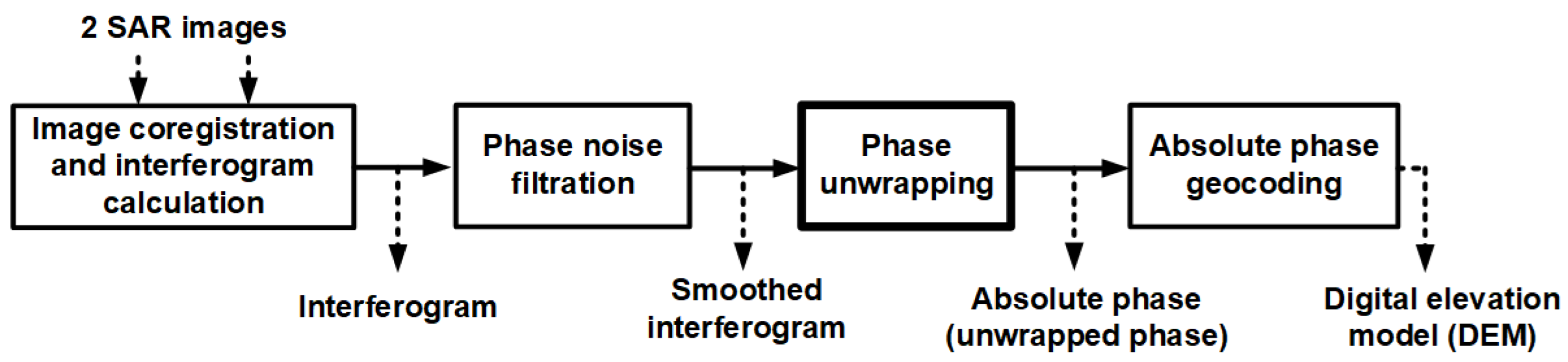
• The topographic phase ${\Psi }_{m,n}$ due to the terrain;
• The phase $\Delta D_{m,n}$ caused by a change in the inclined range due to the displacement of the surface element between shots;
• The phase $\Delta {\varphi }_{math,m,n}$ caused by a change in the conditions of propagation of radio waves in the atmosphere during the period between surveys [1,2];
• Phase noise $\Delta {\varphi }_{noise,m,n}$ caused by a partial loss of coherence of reflected waves due to differences in shooting angles and surface variability during the time between shots during two-pass shooting (spatial and temporal decorrelation).

As a result, the interferometric phase has the following form [1,4]:

$$\begin{array}{c}\Delta {\varphi }_{m,n}\approx W\left\{-{\Psi }_{m,n}-{\displaystyle \frac{4\pi }{\lambda }}\Delta D_{m,n}+\Delta {\varphi }_{atm,m,n}+\Delta {\varphi }_{noise,m,n}\right\}\hfill \\ {\Psi }_{m,n}={\displaystyle \frac{4\pi }{\lambda }}\Delta R_{m,n}={\displaystyle \frac{4\pi }{\lambda }}(R_{1,m,n}-R_{2,m,n}),\hfill \end{array}$$

(1)

where $m,n$ are the coordinates of the interferogram elements, $\Delta R_{m,n}$ is the difference of the minimum (traverse) inclined ranges from the radar to the surface element during the first and second surveys, $\lambda$ is the radar wavelength, and $W\left\{·\right\}$ is the symbolic record of phase wrapping into the range of values $[-\pi ,\pi )$.

The purpose of interferometric processing is to restore the absolute phase ${\widehat{\Psi }}_{m,n}$ by performing the phase unwrapping operation, which implies disclosure of $2\pi$-ambiguity of phase measurements, and suppressing the noise component $\Delta {\varphi }_{noise,m,n}$. The main problems that have to be overcome with interferometric processing, first of all, include the decorrelation of reflected signals and the complexity of phase unwrapping, especially when processing high-resolution radar data containing a large number of phase discontinuity areas (primarily when imaging urban areas, i.e., buildings and structures).

The beginning of research in the field of phase unwrapping can be attributed to the second half of the 1970s. The research was related to the cepstral processing of one-dimensional and two-dimensional signals obtained from astronomical measurements. The first practical results in the field of space radar interferometry were demonstrated in the second half of the 1980s. The development of radar space technologies for remote sensing of the Earth for terrain mapping in the 1980s and 1990s. This led to the development of dozens of new algorithms for the phase unwrapping. The problem of phase unwrapping does not have an unambiguous analytical solution and in practice is solved by approximate methods. The algorithms were developed using the mathematical apparatus of vector field theory (Goldstein Residual Cut method and Green’s function method), optimization theory (integer optimization method and minimum cost flow method [5,6]), filtration theory (Kalman filtration method, nonlinear stochastic filtration method, etc.), solving large systems of linear equations (least squares method), genetic algorithms, neural networks, deep learning techniques, like wrap counting, phase regression, gradient information fusion, etc. [7,8,9,10]. The reviews [1,4,7,11] mention more than 50 different phase unwrapping algorithms. Parallel computing is also actual in the area of the phase unwrapping [12].

In the works [1,6], it is indicated that in the mathematical formulation, the task of phase unwrapping is $NP$-difficult. This significantly complicates the interferometric processing of large images (more than two thousand elements on each side) containing a large number of phase discontinuities (singularities). Many unwrapping algorithms (in particular, the region growing algorithm) are linear in terms of computational complexity, but they leave extensive artifacts. This leads to a deterioration in the accuracy of digital terrain models up to values comparable to the relief approximation by an equivalent plane. The most common algorithm for solving this problem is the minimum cost flow algorithm. It allows one to obtain a solution to the problem that is close to optimal.

Note that most of the unwrapping methods with acceptable accuracy (the minimum flow cost method [6], the brunch-cut method, etc.) have at least quadratic computational complexity, which makes their parallel implementation ineffective or impossible. Methods that allow parallel implementation (the least squares method, Green’s functions, etc.) have insufficient accuracy for practical application. For example, in the works of Aoki [13], Tomioka [14,15], an algorithm suitable for parallel implementation and having linear computational complexity is proposed. This algorithm uses the direct elimination of discontinuity points with the addition of a vortex shape $\delta \overline{\varphi }$ to the interferogram of the following form:

$$\begin{array}{c}\delta \overline{\varphi }=\pm arctg\left\{{\displaystyle \frac{m-m_{0/p}}{n-n_{0/p}}}\right\},\hfill \end{array}$$

(2)

where $m_{0/p}$, $n_{0/p}$ are the coordinates of the singular point where the center of the vortex is placed. After this elimination of discontinuities, the absolute phase is restored using the phase gradient summation. However, this approach leads to an incongruent solution, and in some of the cases, does not allow to obtain a correct solution due to the appearance of residual phase discontinuities.

In the works [16,17], the sequential inverse vortex phase field algorithm and its block implementation were proposed.

In this paper, we propose a new parallel phase unwrapping algorithm, which uses the direct elimination of singular points using a similar model (2). The advantages and novelty of the proposed method of inverse vortex phase field flattening lie in the possibility of its parallel implementation. The algorithm uses recursive alignment of the inverse vortex field and low-frequency filtering, which makes it possible to obtain a congruent solution and significantly reduces phase unwrapping errors. The proposed algorithm solves the problem of phase unwrapping in quasi-linear time and allows the parallelization of calculations. The algorithm is implemented on a multicore processor using OpenMP technology. The properties and characteristics of real interferometric SAR data are investigated. The interferogram models with the appropriate characteristics for efficiency investigation are proposed. Computational experiments are carried out on the proposed models. The efficiency of the algorithm is investigated depending on the dimension of the source data and the number of processor cores.

Section 2 of this article describes the properties and characteristics of the source data. In Section 3, a numerical method for solving the phase unwrapping problem (the IVPF method) is proposed, which approximately solves the unwrapping problem in quasi-linear time. A block diagram of the numerical method is given. In Section 4, a parallel phase unwrapping algorithm is developed and described based on the numerical method of solving the problem. Section 5 presents the results of numerical experiments to evaluate the effectiveness of the algorithm when implemented on a multicore processor using OpenMP technology.

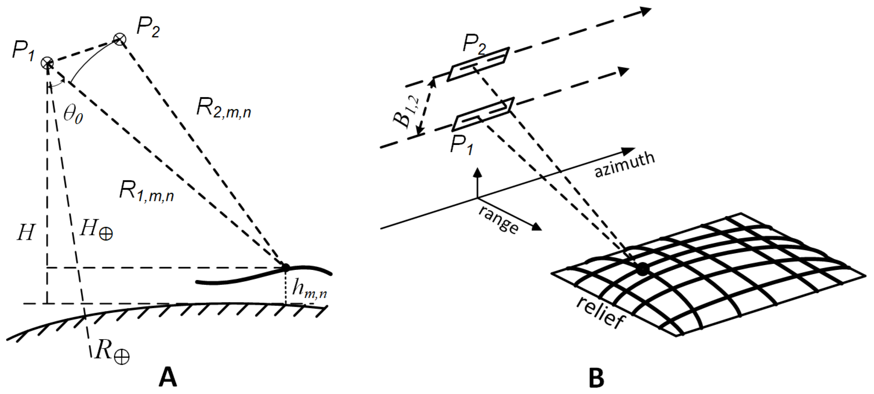
2. Source Data for the Problem

Interferograms of space radar systems for the remote sensing of the Earth are two-dimensional random processes (images), the characteristic feature of which is interference fringes. The fringe boundaries correspond to the breakout of phase differences by $2\pi$ value (or to a change in the difference distance by $4\pi \Delta R/\lambda$ value) and depend on the geometric characteristics of the system and the terrain. Examples of interferograms of the ALOS PALSAR spacecraft are shown in Figure 3).

Phase unwrapping is the main stage of interferometric processing of Earth radar sensing data. As a result of its execution, the resulting phase pattern begins to repeat the shape of the relief of the surface area from which the radar signal was received. When the phase is unwrapped, the interference fringes of the relative phase $\Delta {\varphi }_{m,n}$ are “stitched” into the picture of the absolute phase ${\widehat{\Psi }}_{m,n}$ (Figure 4). The main approach to solving this problem is to sum the phase gradient along a trajectory covering all the elements of the interferogram:

$$\begin{array}{c}\delta {\varphi }_{m,n}=W\left\{\Delta {\varphi }_{m,n}-\Delta {\varphi }_{m-m_i,n-n_j}\right\},\hfill \\ {\Psi }_{m,n}=\delta {\varphi }_{m,n}+\delta {\varphi }_{m-i,n-j},\hfill \end{array}$$

(3)

The result of such unwrapping will be correct only if there are no phase gaps in the interferogram. A phase gap, as a rule, is a certain line on an arbitrary trajectory. In the presence of the gap area, the unwrapping results depend on the direction of phase differences summation $\delta {\varphi }_{m,n}$ [4]. The gap is bordered by singular points (phase gap points), where the condition of equality of the sum of phase differences on an elementary closed contour is violated

$$\begin{array}{c}{Q}_{m,n}=W\{\Delta {\varphi }_{m,n}-\Delta {\varphi }_{m-1,n}\}+W\{\Delta {\varphi }_{m-1,n}-\Delta {\varphi }_{m-1,n-1}\}+\hfill \\ +W\{\Delta {\varphi }_{m-1,n-1}-\Delta {\varphi }_{m,n-1}\}+W\{\Delta {\varphi }_{m-1,n}-\Delta {\varphi }_{m,n}\},\hfill \end{array}$$

(4)

where $Q_{m,n}$ is a residue function, which is other than zero at the interferogram singular points and calculated according to rules similar to the rules for calculating the deductions of functions of a complex variable. The singular points occur on the interferogram, as a rule, in pairs. An error occurs when crossing the line connecting them when unwrapping according to the rule (3). The error lies in the appearance or omission of one interference band (Figure 5). The absolute phase in such a situation, in principle, cannot be unambiguously restored [1,4].

Effective phase unwrapping algorithms should form a solution to the unwrapping problem in which phase unwrapping artifacts are localized in the smallest possible neighborhood of the phase gap area. In the next section, we propose a method for equalizing the inverse vortex phase field (IVPF), which allows us to localize artifacts in the vicinity of the rupture, and at the same time has quasi-linear accuracy.

3. Numerical Method for Problem Solving

The proposed sequential method of equalization of the inverse vortex field of the phase is based on the direct elimination of interferogram discontinuities by artificial discontinuities (elementary phase vortices) of the inverse direction [16]. A set of artificial discontinuities forms an inverse vortex field of the phase. Next, the recursive alignment of this field and its adaptive filtering are performed.

The interferogram in the description of the method is described as an argument to a function of a complex variable $\dot{I}\left(z\right)=exp\left\{\delta {\varphi }_{m,n}\right\}{|}_{z=m+jn}$. The continuity of the phase can be restored if a zero of the complex variable q of the order is artificially placed at each singular point of the interferogram q of the positive sign, and a pole of the complex variable q of the order is placed at the singular point with a negative sign. In this case, the inverse vortex field of the interferogram phase has the form

$${\dot{C}}_{\ast }\left(z\right)=exp\left(j·arg\left\{{\displaystyle \frac{{(z-z_{p1})}^{q_{p1}}{(z-z_{p2})}^{q_{p2}}···{(z-z_{p\mu })}^{q_{p\mu }}}{{(z-z_{01})}^{q_{01}}{(z-z_{02})}^{q_{01}}···{(z-z_{0u})}^{q_{0\nu }}}}\right\}\right),$$

(5)

where $\mu ,\nu$ are the numbers of the interferogram singular points of the positive and negative signs, respectively; $q_{pi}$ is the order of the i-th pole; and $q_{0j}$ is the order of the j-th zero. Multiplication of the complex interferogram $\dot{I}\left(z\right)$ by the inverse vortex field ${\dot{C}}^{\ast }\left(z\right)$ should lead to the disappearance of singular points and the formation of a discontinuous relative phase. After that, the final unwrapping could be performed by summing the differences along any trajectory on the interferogram. The differences should be collapsed into a phase ambiguity interval $[-\pi ,\pi )$. So, the absolute phase ${\tilde{\Psi }}_{m,n}$ (see Figure 6) is as follows:

$${\tilde{\Psi }}_{m,n}={\mathrm{{\rm Y}}}_r\left\{arg\{\dot{I}\left(z\right)·{\dot{C}}_{\ast }\left(z\right)\}{|}_{z=m+jn}\right\},$$

(6)

where ${\mathrm{{\rm Y}}}_r\{·\}$ is the symbolic designation of the unwrapping according to the rule (3) of summing the differences of neighboring interferogram elements.

However, due to the discrete nature of the interferogram and the quantization of phase values, after such multiplication, new singular points may appear or move to new positions. To compensate for them, it is proposed to calculate the deduction function $Q_{m,n}^{II}$ again, form a new inverse vortex field ${\dot{C}}_{II}\left(z\right)$ and re-apply multiplication to a new vortex field. The procedure for such formation of the inverse phase field vortex is carried out iteratively until all phase discontinuities are completely eliminated.

The final inverse vortex field of the phase $C_{\ast \ast }\left(z\right)$ will be the product of the inverse vortex fields obtained in separate iterations of the algorithm and will have the following form:

$${\dot{C}}_{\ast \ast }\left(z\right)={\dot{C}}_I\left(z\right)·{\dot{C}}_{II}\left(z\right)·{\dot{C}}_{III}\left(z\right)·\dots ·{\dot{C}}_{K_{Itrs}}\left(z\right),$$

(7)

where ${\dot{C}}_I\left(z\right),{\dot{C}}_{II}\left(z\right),\dots$ are the inverse vortex fields obtained in the first, second and subsequent iterations of the algorithm, and $K_{Itrs}$ is the number of iterations. Next, the absolute phase is formed according to the rule (6).

In order to increase the accuracy of the absolute phase and restore small relief details, it is proposed in this work to restore the congruence of the absolute phase by adding a residual interferogram (residual phase):

$${\dot{I}}_{\delta }\left(z\right)=\dot{I}\left(z\right)/e^{j{\tilde{\Psi }}_{m,n}}{|}_{z=m+jn}=-arg{\dot{C}}_{\ast \ast }\left(z\right)$$

(8)

to the continuous absolute phase ${\tilde{\Psi }}_{m,n}$

$${\widehat{\Psi }}_{m,n}={\tilde{\Psi }}_{m,n}+arg\left\{{\dot{I}}_{\delta }\left(z\right){|}_{z=m+jn}\right\}.$$

(9)

However, for interferograms of areas with rough terrain, a large number of extended phase discontinuities occur, the lines of which will be located randomly on the residual interferogram $arg\left\{{\dot{I}}_{\delta }\left(z\right)\right\}$. This leads to a number of problems that reduce the accuracy of the obtained result (low-frequency fluctuations, etc.). To overcome these problems, it is proposed to align the vortex field of the interferogram in such a way that the phase discontinuity lines have a minimum length. For this purpose, the recursive formation of the residual interferogram is used, which is carried out as follows.

After the first iteration of constructing the inverse vortex field according to the rules (5) and (6) using a two-dimensional low-pass Gaussian filter, the low-frequency component of the phase of the resulting inverse vortex field ${\dot{E}}_{Ir.1}\left(z\right)$ is allocated. As a rule, it also contains gaps. For this component, the inverse vortex field ${\dot{C}}_{Ir.2}\left(z\right)$ is constructed again, from which the low-frequency component is again isolated. In this case, the cutoff frequency of the amplitude–frequency response (frequency response) $F_i$ of the filter is set several times lower than in the previous step. The recursive descent with a gradual decrease in the frequency of the frequency response of the filter continues until a continuous interferogram is obtained:

$$\begin{array}{c}{\dot{C}}_{Ir.1}\left(z\right)={\mathrm{{\rm Y}}}_v\left\{\dot{I}\left(z\right)\right\}\hfill \\ {\dot{E}}_{Ir.1}\left(z\right)={\Omega }_{\gamma 1}\left\{{\dot{C}}_{Ir.1}\left(z\right)\right\}\hfill \\ {\dot{C}}_{Ir.2}\left(z\right)={\mathrm{{\rm Y}}}_v\left\{{\dot{E}}_{Ir.1}\left(z\right)\right\}\hfill \\ {\dot{E}}_{Ir.2}\left(z\right)={\Omega }_{{\gamma }_2}\left\{{\dot{C}}_{Ir.2}\left(z\right)\right\}\hfill \\ \dots \hfill \\ {\dot{E}}_{Ir.K_{I-Rc}}\left(z\right)={\Omega }_{\gamma K_{I-Rc}}\left\{C_{Ir.K_{I-Rc}-1}\left(z\right)\right\},\hfill \end{array}$$

(10)

where ${\mathrm{{\rm Y}}}_v\{·\}$ is the symbolic designation of the construction of an inverse vortex field in accordance with the Formula (6); ${\Omega }_{\gamma i}\{·\}$ is the symbolic designation of low-frequency Gaussian filtering with a cutoff frequency filter frequency response $F_i$; ${\dot{C}}_{Ir.i}\left(z\right)$ are inverse vortex fields after i-x recursion steps, ${\dot{C}}_{Ir.1}\left(z\right)={\dot{C}}_I\left(z\right)$, ${\dot{E}}_{Ir.1}\left(z\right)$ are low-frequency components of inverse vortex fields, $K_{I-Rc}$ is the depth of recursive descent at the I iteration. From these vortex fields, the inverse vortex field of the first iteration of the algorithm is formed

$$\begin{array}{c}{\dot{C}}_{\text{I-Rc}}\left(z\right)={\displaystyle \frac{{\dot{C}}_{Ir.1}\left(z\right)}{{\dot{E}}_{Ir.1}\left(z\right)}}·{\displaystyle \frac{{\dot{C}}_{Ir.2}\left(z\right)}{{\dot{E}}_{Ir.2}\left(z\right)}}·\dots ·{\displaystyle \frac{1}{{\dot{E}}_{{\mathrm{Ir}.\mathrm{K}}_{\text{I-Rc}}}\left(z\right)}}.\hfill \end{array}$$

(11)

Similarly, an inverse vortex field is constructed in the following iterations of the algorithm. The absolute phase is calculated according to the rule (9). When calculating the residual interferogram, the product of the inverse vortex fields at all recursive transitions is used

$$\begin{array}{c}\dot{C}\left(z\right)={\dot{C}}_{\text{I-Rc}}\left(z\right){\dot{C}}_{\text{II-Rc}}\left(z\right)\dots {\dot{C}}_{\text{N-Rc}}\left(z\right).\hfill \end{array}$$

(12)

As a result of the application of recursive processing, the inverse vortex field has a noticeably lower level of low-frequency fluctuations (Figure 7A,B). This leads to a significant reduction in phase unwrapping errors.

The proposed method of phase unwrapping based on the alignment of the inverse vortex field of the phase (IVPF method) is implemented as an algorithm. The steps of the algorithm are as follows:

(0)

Initialization of input data and parameters: interferogram $\dot{I}\left(z\right)$ and frequency response of the filter $F_S$.

(1)

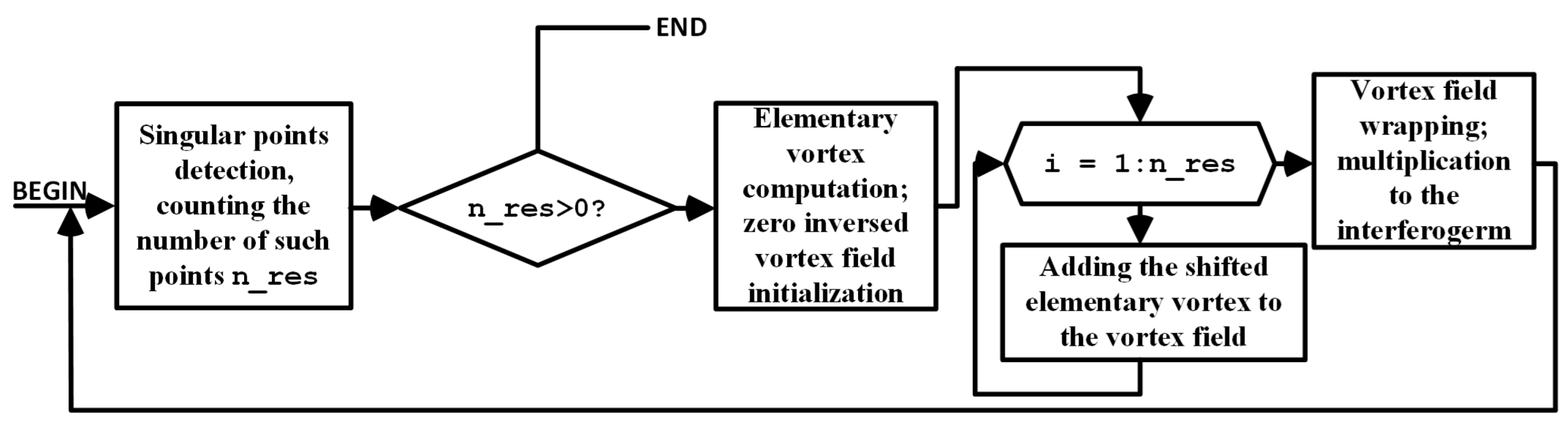
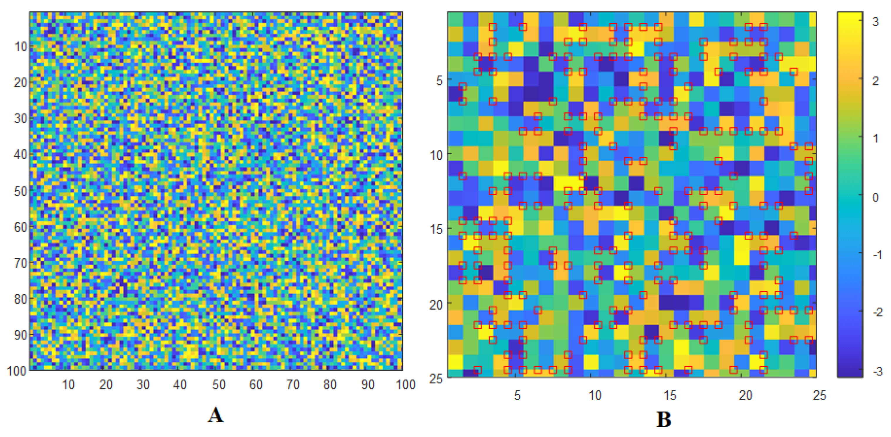
Detection of singular points (calculation of the interferogram residue function $Q_{m,n}$ using Formula (4) and counting their number $\mu +\nu$. If $\mu +\nu =0$, then go to step 6.

(2)

Calculation of the inverse vortex field $\dot{C}\left(z\right)$ by the Formula (5).

(3)

Filtering of the field $\dot{C}\left(z\right)$, obtaining a smoothed inverse vortex field $\dot{E}\left(z\right)$ using the Formula (10).

(4)

Calculation of the number of singular points of the smoothed inverse vortex field ${\mu }_E+{\nu }_E$. If ${\mu }_E+{\nu }_E=0$, then we accept the inverse vortex field $\dot{C}\left(z\right)$ equal to the smoothed $\dot{E}\left(z\right)$. Otherwise, we return to step 0 with the input arguments $F_S/4$, $\dot{I}\left(z\right)\dot{C}\left(z\right)/\dot{E}\left(z\right)\to \dot{I}\left(z\right)$.

(5)

Calculation of the continuous absolute phase according to Formula (6) and the residual interferogram according to Formula (8).

(6)

Calculation of the unwrapped interferogram according to Formula (9).

The calculations in step 2 (“unwrap3” sub-algorithm) are the most time-consuming and take up most of the time of the entire algorithm.

In Figure 8, a simplified block diagram of the unwrapping algorithm is presented.

The performance of the proposed algorithm was previously compared with widely used phase unwrapping algorithms: minimum cost flow, Green’s functions and least squares. These methods are most often used in specialized software (SARscape, PHOTOMOD RADAR, ESA SNAP, etc.). The results show that the proposed algorithm and minimum cost flow are compared in accuracy for medium-sized interferograms. Green’s functions and the Least squares algorithms are less accurate (20% using the root mean square error criterion RMSE). For big-size interferograms, the proposed algorithm exceeds the minimum cost flow algorithm (up to 15–20% in RMSE) due to its capability to process the whole interferogram without decomposition.

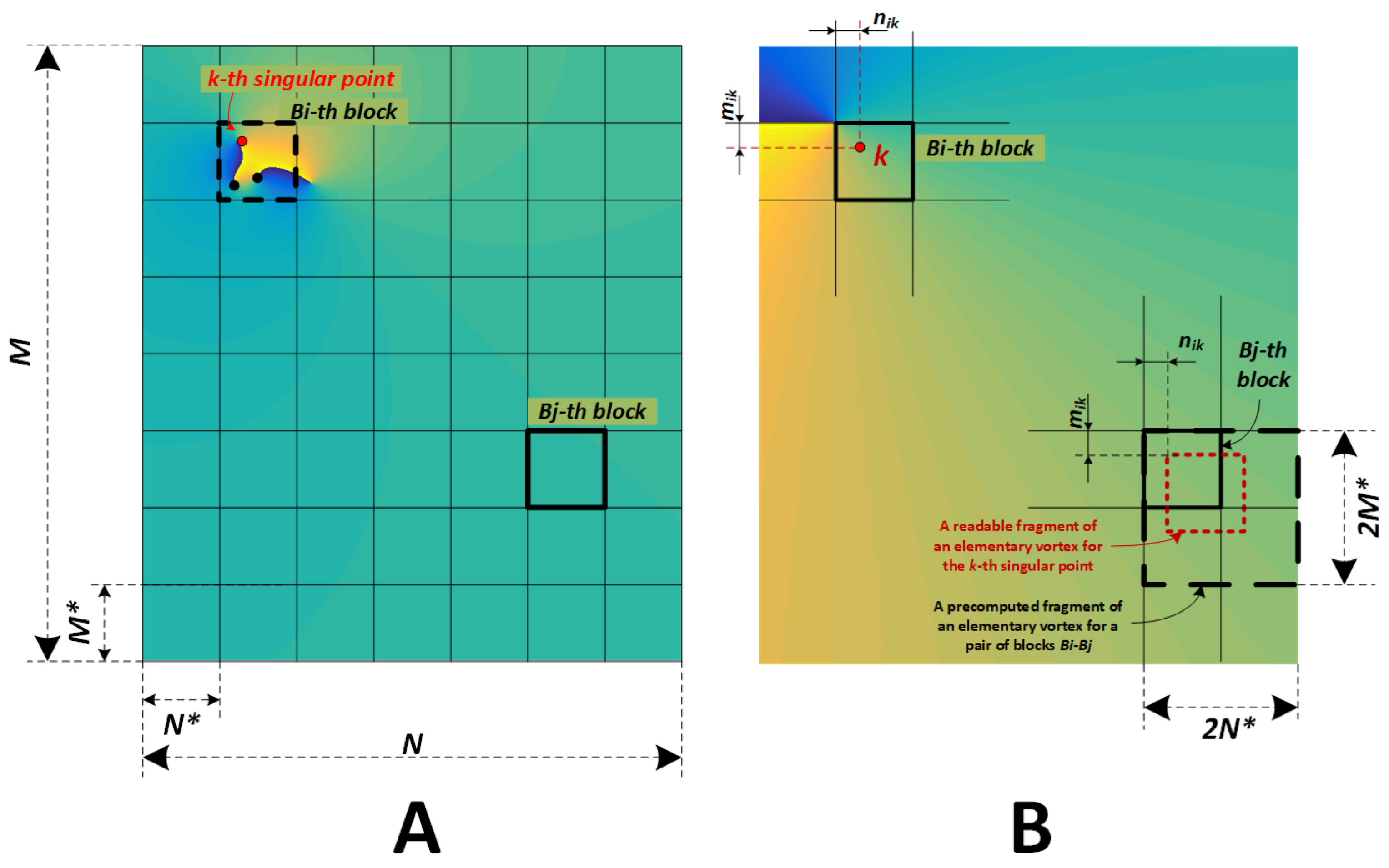
4. Parallel Implementation of the Numerical Algorithm

The sub-algorithm for constructing an inverse vortex field can be implemented on parallel computing devices since the operations of constructing elementary vortices for individual discontinuity points are performed independently of each other, while the discontinuity points can be traversed in any order. To process large-sized interferograms, the authors proposed [17], a block implementation of the algorithm. It consists in dividing the interferogram into small blocks, constructing an inverse vortex field separately and independently for each block, which is implemented as follows.

The calculation of the inverse vortex field (for the “unwrap3” algorithm) is the most computationally intensive procedure in the entire algorithm and takes up to 90% of its operation time. So, it is reasonable to use parallel calculations for its implementation. The parallel implementation of the “unwrap3” sub-algorithm was first proposed in [17] and can be implemented on two levels. The results of the calculations of block and non-block implementations are identical, which is not always achievable for other phase unwrapping algorithms (i.e., the minimum cost flow algorithm).

At the first level, calculations are parallelized by singular points throughout the entire interferogram. The operations of constructing elementary vortices when calculating the inverse vortex phase field for individual singular points can be performed independently of each other. In this case, the bypass of the singular points can be performed in any order since the calculation operations are commutative and associative. Therefore, the “unwrap3” subalgorithm can be implemented in parallel computing systems. When calculating the vortex field over the entire interferogram, exchange operations between processors are not required. This reduces the time required to perform field calculations on a multicore processor, but a large amount of memory is required.

At the second level, to reduce the amount of memory when processing large interferograms, it is proposed to use splitting the interferogram into small blocks B. To calculate the field in each j block ($B_j$), it is required to use positions of singular points from all blocks $B_i$ (including cases when $i=j$), $i,j=\overline{1,K_B}$, where $K_B$ is the number of blocks. In this case, the construction of the inverse vortex field is implemented as follows.

• The entire interferogram of size $M\times N$ pixels is divided into blocks B of small size $M^{\ast }\times N^{\ast }$ pixels. The optimal block size is selected experimentally. On the one hand, the block and auxiliary data must fit entirely into the system’s RAM. On the other hand, increasing the number of blocks should not significantly slow down calculations.
• In each i-th block ($B_i$), the residue function (4) is calculated, and the coordinates of the singular points are determined $\left(m_{ik},n_{ik}\right)$ (Figure 9).
• In each j-th block, the fragment of an elementary vortex $J^{\ast }\left(z\right)$ of size $2M^{\ast }\times 2N^{\ast }$ is calculated, the break point of which is located in the upper left corner of the i-th block, and the boundaries cover the j-th block. When calculating the inverse vortex field in the j-th block from the singular point k with coordinates $\left(m_{ik},n_{ik}\right)$ lying in the i block, a fragment of the elementary vortex $J^{\ast }\left(z\right)$ of the size of $M^{\ast }\times N^{\ast }$ shifted by $\left(m_{ik},n_{ik}\right)$ relative to the upper-left corner is read. The contents of the read fragment are added to the previously calculated inverse vortex field.
• Step 3 is repeated until all singular points in block $B_i$ have been passed.
• Steps 3–4 are repeated until all pairs of blocks $B_i-B_j$ have been processed.
• The inverse vortex fields of size $M^{\ast }\times N^{\ast }$, calculated in all blocks $B_j$, are joined into a united inverse vortex field of size $M\times N$.

Figure 9. Calculation of the inverse vortex field of the phase with a block implementation of the unfolding algorithm: (A) splitting the interferogram; (B) elementary vortex for block $B_i$ and calculation of a fragment of the inverse vortex field from the singular point k in block $B_j$.

Figure 9. Calculation of the inverse vortex field of the phase with a block implementation of the unfolding algorithm: (A) splitting the interferogram; (B) elementary vortex for block $B_i$ and calculation of a fragment of the inverse vortex field from the singular point k in block $B_j$.

The block implementation does not use approximations, allowing one to obtain the same result in constructing an inverse vortex field as the original IVPF algorithm. It reduces the memory requirements of computing devices since the size of an elementary vortex when using it becomes equal to $2M^{\ast }\times 2N^{\ast }$ (four times the block size). The speed of the parallel implementation of the algorithm is proportional to the square of the number of interferogram blocks.

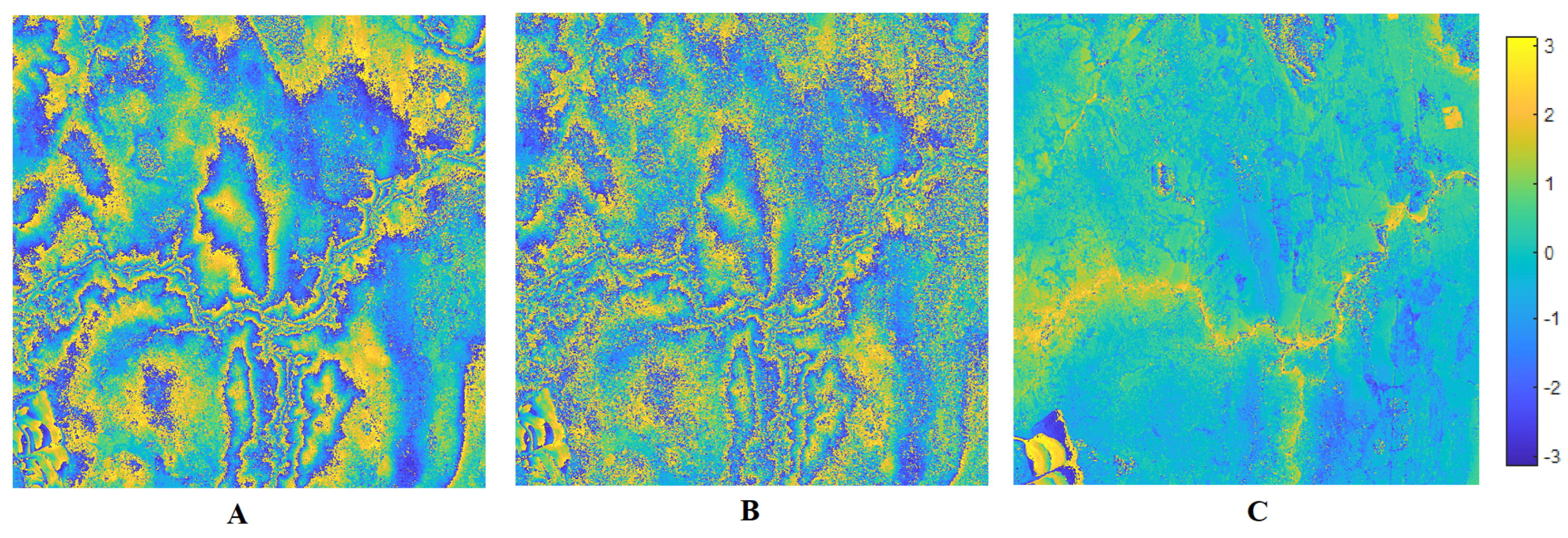
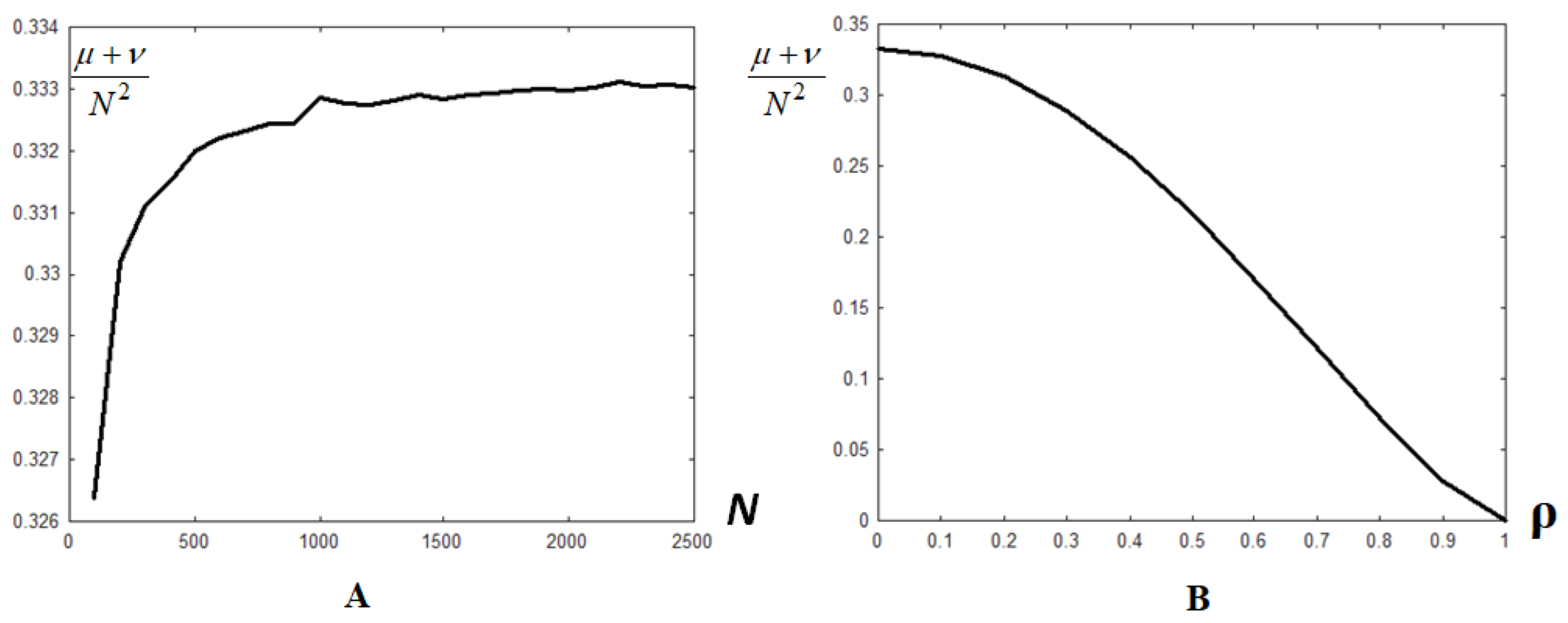
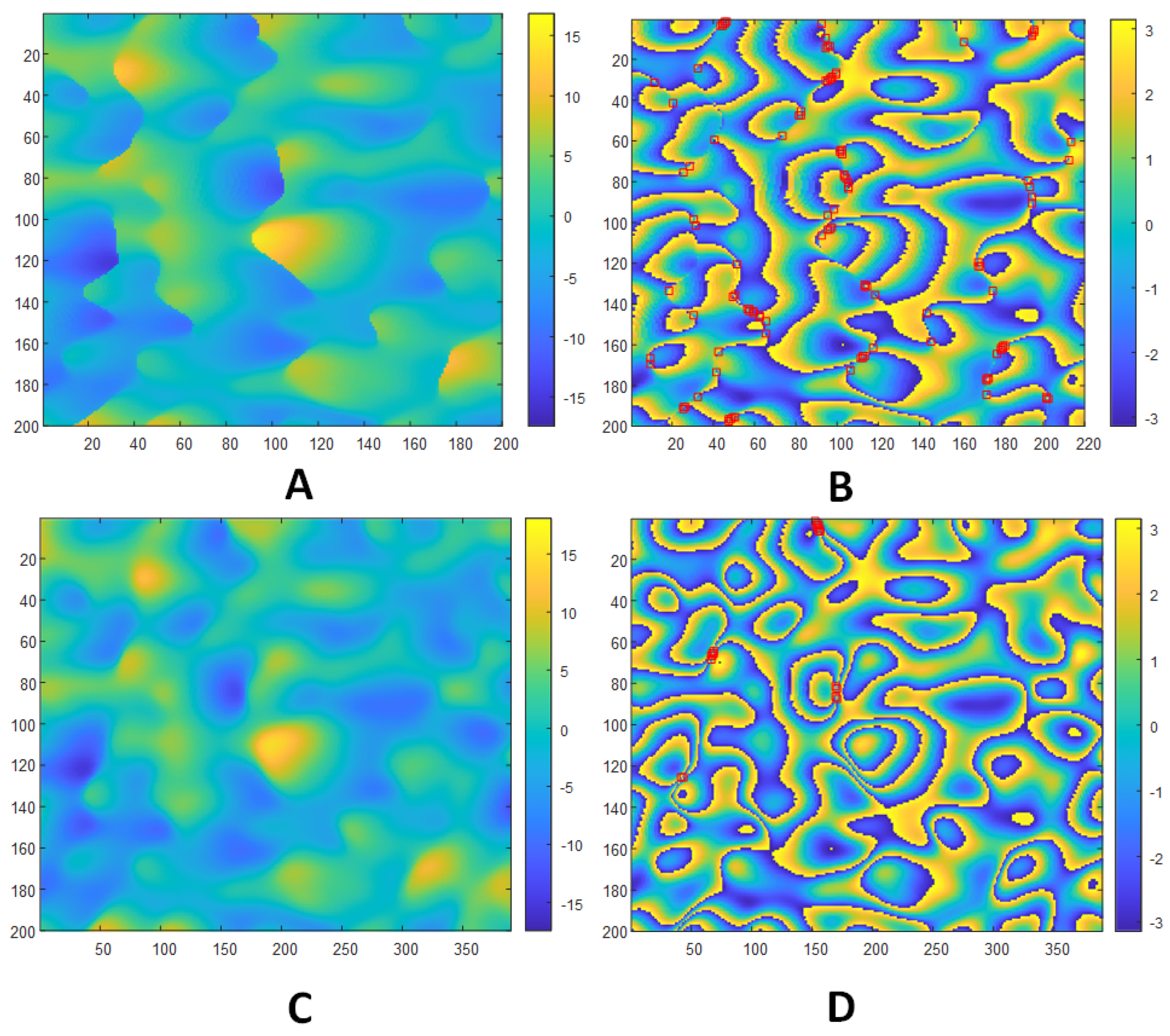
5. Numerical Experiments for Interferogram Models and OpenMP Performance

In the works [1,4], a classification of interferometric phase discontinuities is proposed, depending on the sources of origin and the forms of their manifestation on the interferogram. To solve problems related to evaluating the performance of phase unwrapping algorithms, it is proposed to use the following models of interferograms with phase discontinuities.

Data Models

A. A “rough surface” model is a flat surface with full or partial decorrelation of echo signals. The model is described as follows:

$${\Psi }_{m,n}=arg\{{\dot{X}}_{1,m,n}·X_{2,m,n}^{\ast }\},$$

(13)

where ${\dot{X}}_{1,m,n}$ is a complex uncorrelated Gaussian discrete random process, and ${\dot{X}}_{2,m,n}$ is a complex Gaussian discrete random process having a correlation coefficient with the process ${\dot{X}}_{1,m,n}$. It is obtained as follows:

$$X_{2,m,n}^{\ast }=\rho {\dot{X}}_{1,m,n}+\sqrt{1-{\rho }^2}{\dot{X}}_{20,m,n},$$

(14)

where ${\dot{X}}_{20,m,n}$ is a complex uncorrelated Gaussian discrete random process. This process is uncorrelated with the process ${\dot{X}}_{1,m,n}$. $\rho =0$ corresponds to a complete decorrelation of echo signals (phase noise, see Figure 10). $\rho \in (0,1)$ corresponds to a partial decorrelation. The density of singular points in the full decorrelation case ${\displaystyle \frac{\mu +\nu }{NM}}=1/3$ (Figure 11A). As the correlation coefficient increases, the average density of singular points decreases (Figure 11B).

This model makes it possible to estimate the computational time of phase unwrapping algorithms. It allows one to control the interferogram size and the number of singular points. At the same time, the model does not allow estimating the accuracy of phase unwrapping.

B. A “random smooth surface” model in an equidistant projection. It represents a random discrete low-frequency Gaussian field $H(m^{\prime },n^{\prime })$ with an amplitude spectral density of the form

$$S_{k,l}=exp\left\{-{\displaystyle \frac{1}{2}}\left[{\left({\displaystyle \frac{k-M/2}{F_S}}\right)}^2+{\left({\displaystyle \frac{l-N/2}{F_S}}\right)}^2\right]\right\},$$

(15)

where N and M are interferogram sizes, $k=\overline{1..M}$ and $l=\overline{1..N}$ are the spectral density sampling indices, and $F_S$ is the spectral density cutoff frequency (upper boundary frequency of the process). The transformation of the model into an equidistant projection, typical for side-view radars, is carried out as follows.

At first, the ranges $R(m^{\prime },n^{\prime })$ are calculated for each element of the model:

$$R(m^{\prime },n^{\prime })=\sqrt{{(H_B-H(m^{\prime },n^{\prime }))}^2+{(L_B+n^{\prime })}^2},$$

(16)

where $H_B$ is the height of the orbit; $L_B$ is the ground range from the satellite point to the nearest edge of the model; and $m^{\prime },n^{\prime }$ are pixel coordinates of the model elements before conversion to an equidistant projection, where $m^{\prime }$ is the line number, $n^{\prime }$ is the column number. Then, the coordinates of the model elements are converted so that the column number corresponds to the number of the radar range channel, and the row number does not change. So, we have

$$\begin{array}{c}m=m^{\prime },\hfill \\ n=\left[{\displaystyle \frac{R_1(m^{\prime },n^{\prime })-R_{min}}{\delta R}}\right],\hfill \end{array}$$

(17)

where $R_{min}$ is the minimum inclined range, and $\delta R$ is the spatial resolution of the radar along the inclined range. The absolute phase $\Delta {\Psi }_{m,n}$ for the model is calculated as follows:

$$\Delta {\Psi }_{m,n}={\displaystyle \frac{4\pi B_{\perp }H(m,n)}{\lambda R(m,n)sin{\theta }_0}},$$

(18)

where ${\theta }_0$ is the inclination angle, and ${\theta }_0\approx atan(L_B/H_B)$, $B_{\perp }$ is the length of the projection of the interferometric baseline on the slant range direction. The conversion of the absolute phase into the interferogram of the model is carried out by the operation of phase wrapping

$$\Delta {\varphi }_{m,n}=W\left\{{\Psi }_{0,m,n}\right\},$$

(19)

where $W\left\{{\Psi }_{0,m,n}\right\}$ is the operation of the phase wrapping into the range of values $[-\pi ,\pi )$. The model examples of absolute phases $\Delta {\Psi }_{m,n}$ and corresponding interferograms $\Delta {\varphi }_{m,n}$ for different inclination angles ${\theta }_0$ are shown in Figure 12. Low inclination angles lead to the appearance of the foreshortening phenomenon, which produces phase gaps and singular points. As the inclination angle increases, the number of singular points decreases.

The “random smooth surface” model allows one to estimate both the accuracy of the phase unwrapping and computational speed of the unwrapping algorithms. On the other hand, the number of singular points in this case is less predictable.

The numerical experiments for the phase unwrapping consist in the execution of the IVPF algorithm (5)–(12) over the model interferograms under different conditions (number of interferogram elements N, number of singular points $\mu +\nu$, interferogram smoothness).

The experiments were performed on an Intel(R) Core(TM) i7-8700 processor (3.2 GHz, 6 cores) using the MSVC compiler of the MS Visual Studio 2022 under Windows 10 operating system. The initial data had a size of $750\times 750$ elements and approximately 187,000 singular points. The results of the computation are adequate for the uncorrelated surfaces of SAR images.

The complexity of the IVPF algorithm has the form of $O(N·M·(\nu +\mu \left)\right)$. So, the computing time for the algorithm is proportional to the number of interferogram elements and the singular points. For real SAR image data, the interferogram size may exceed several tens of thousands of elements on each interferogram side, so the execution time may be several days.

1. Experiment consisted in the parallelization of the ”unwrap3” algorithm and reducing the computational time of the whole IVPF phase unwrapping algorithm using the “rough surface model A” under different parameters.

For studying the threading performance, we used the speedup $S_m=T_1/T_m$ and efficiency $E_m=S_m/m$ coefficients, where $T_m$ is the computing time on m OpenMP threads for the same problem.

Table 1. Performance for the model A ($750\times 750$ elements, 187,000 singular points).

Number m of OpenMP Threads	Time ${\mathit{T}}_{\mathit{m}}$ [min.]	Speedup ${\mathit{S}}_{\mathit{m}}$	Efficiency ${\mathit{E}}_{\mathit{m}}$
1	59.8	—	—
2	29.9	2.00	1.00
6	16.0	3.75	0.62
12	10.7	5.60	0.47

shows the results of solving the problem on various numbers of the OpenMP threads for the “rough surface model A”. The table contains the computing times of the algorithm, speedup and efficiency coefficients.

A speedup of 5.6 times on the 6-core processor was achieved. Using the parallel algorithm reduces the computing time proportional to the square root of the number of threads.

The further increase in the number of threads leads to longer computations due to increased data exchange between threads and RAM limitations. The minimum computing time is obtained with 12 threads for a 6-core processor (2 threads per core). In the future, to further reduce computing time, we plan to develop a parallel algorithm for a graphics processor (GPU) containing several thousand processor cores.

2. Experiment consisted in measuring both accuracy ${\sigma }_{\Psi }$ and computational speed for the IVPF algorithm using the model “random smooth surface” model. An example of such unwrapping is shown in Figure 13. The initial data had the size of $1000\dots 5000$ elements per each side and approximately 50,000 singular points. The accuracy ${\sigma }_{\Psi }$ of the unwrapped phase was about 1.2 radians.

Table 2. Performance of model B (approximately 50,000 singular points).

Interferogram Number	Number m of OpenMP Threads	Time ${\mathit{T}}_{\mathit{m}}$ [min]	Speedup ${\mathit{S}}_{\mathit{m}}$	Acurracy ${\mathit{\sigma }}_{\mathit{\Psi }}$ [Radians]
1	1	13.8	—	1.27
($1000\times 1000$)	12	2.7	5.1	1.27
2	1	64.3	—	1.22
($2500\times 2500$)	12	12.6	5.1	1.22
3	1	298	—	1.19
($5000\times 5000$)	12	53.3	5.6	1.19

shows the results of solving the problem on various numbers of the OpenMP threads for the “random smooth surface” model. The table contains the computing times of the algorithm, speedup and efficiency coefficients.

6. Conclusions

In this work, we construct the numerical method and the parallel algorithm for interferometric phase unwrapping for the radar remote sensing of the Earth systems. The method is based on the iterative computation of the inverse vortex phase field for the elimination of phase gaps on the interferogram. The advantages and novelty of the proposed method lie in its low (quasi-linear) computational complexity, high accuracy, and the possibility of its parallel implementation. For the large-sized interferograms (more than $2000\times 2000$ elements) processing, dividing the interferogram into independent blocks is proposed. For analysis of the computational efficiency, the “rough surface model” and “smooth surface model” are proposed. The parallel algorithm is implemented using a multicore processor and OpenMP technology. The speedup of 5.1 … 5.6 times on the 6-core processor for the algorithm is achieved. It is shown that parallel implementation does not affect the accuracy of the unwrapping method.

The further plans consist in the realization of the algorithm on the graphic processors (GPUs) for interferometric phase unwrapping with the big data.

References

- Hanssen, R.F. Radar Interferometry. Data Interpretation and Error Analysis; Kluwer Academic Publishers: Dordrecht, Germany, 2002; pp. 81–113. [Google Scholar]
- Verba, V.S.; Neronskiy, L.B.; Osipov, I.G.; Turuk, V.E. Space-Borne Earth Surveillance Radar Systems. Moscow: Radio Engineering; Radiotechnika: Moscow, Russia, 2010; pp. 475–485. [Google Scholar]
- Zhang, T.; Zhang, X.; Li, J.; Xu, X.; Wang, B.; Zhan, X.; Xu, Y.; Ke, X.; Zeng, T.; Su, H.; et al. SAR Ship Detection Dataset (SSDD): Official Release and Comprehensive Data Analysis. Remote Sens. 2021, 13, 3690. [Google Scholar] [CrossRef]
- Rosen, P.A.; Hensley, S.; Joughin, I.R.; Li, F.K.; Madsen, S.N.; Rodriguez, E.; Goldstein, R.M. Synthetic Aperture Radar Interferometry. IEEE Proc. 2000, 88, 33–82. [Google Scholar] [CrossRef]
- Constantini, M. A novel phase unwrapping method based on network programming. IEEE Trans. Geosci. Remote Sens. 1998, 36, 813–821. [Google Scholar] [CrossRef]
- Chen, C.W.; Zebker, H.A. Network approaches to two-dimensional phase unwrapping: Intractability and two new algorithms. J. Opt. Soc. Am. A Opt. Image Sci. Vis. 2000, 17, 401–414. [Google Scholar] [CrossRef]
- Wang, K.; Kemao, Q.; Di, J.; Zhao, J. Deep learning spatial phase unwrapping: A comparative review. Adv. Photonics Nexus 2022, 1, 014001. [Google Scholar] [CrossRef]
- Li, L.; Zhang, H.; Tang, Y.; Wang, C.; Gu, F. InSAR Phase Unwrapping by Deep Learning Based on Gradient Information Fusion. IEEE Geosci. Remote Sens. Lett. 2022, 19, 4502305. [Google Scholar]
- Wu, C.; Qiao, Z.; Zhang, N.; Li, X.; Fan, J.; Song, H.; Ai, D.; Yang, J.; Huang, Y. Phase unwrapping based on a residual en-decoder network for phase images in Fourier domain Doppler optical coherence tomography. Biomed. Opt. Express 2020, 11, 1760–1771. [Google Scholar] [CrossRef] [PubMed]
- Wang, K.; Li, Y.; Kemao, Q.; Di, J.; Zhao, J. One-step robust deep learning phase unwrapping. Opt. Express 2019, 27, 15100–15115. [Google Scholar] [CrossRef] [PubMed]
- Yu, H.; Lan, Y.; Yuan, Z.; Xu, J.; Lee, H. Phase Unwrapping in InSAR. A review. IEEE Geosci. Remote Sens. Mag. 2019, 7, 40–58. [Google Scholar] [CrossRef]
- Gao, J.; Jiang, H.; Sun, Z.; Wang, R.; Han, Y. A Parallel InSAR Phase Unwrapping Method Based on Separated Continuous Regions. Remote Sens. 2023, 15, 1370. [Google Scholar] [CrossRef]
- Aoki, T.; Sotomaru, T.; Ozawa, T.; Komiyama, T.; Miyamoto, Y.; Takeda, M. Two-dimensional phase unwrapping by direct elimination of rotational vector fields from phase gradients obtained by heterodyne techniques. Opt. Rev. 1998, 5, 374–379. [Google Scholar] [CrossRef]
- Tomioka, S.; Heshmat, S.; Miyamoto, N.; Nishiyama, S. Phase unwrapping for noisy phase maps using rotational compensator with virtual singular points. Appl. Opt. 2010, 49, 4735–4745. [Google Scholar] [CrossRef]
- Heshmat, S.; Tomioka, S.; Nishiyama, S. Performance Evaluation of Phase Unwrapping Algorithms for Noisy Phase Measurements. Int. J. Optomechatronics 2014, 8, 260–274. [Google Scholar] [CrossRef]
- Sosnovsky, A.V.; Kobernichenko, V.G. An InSAR phase unwrapping algorithm with the phase discontinuity compensation. CEUR Workshop Proc. 2017, 2005, 127–136. [Google Scholar]
- Sosnovsky, A.V.; Kobernichenko, V.G. Processing of large-size InSAR images: Parallel implementation of inverse vortex phase field algorithm. CEUR Workshop Proc. 2018, 2274, 75–81. [Google Scholar]