Application of Complex Neutrosophic Graphs in Hospital Infrastructure Design

Abstract

Complex neutrosophic graphs are created by combining complex neutrosophic sets with graph theory ideas. This provides a flexible framework for tackling complex problem-solving circumstances. Various processes, such as union, join, and composition, are thoroughly investigated to improve the administration of complicated neutrosophic graphs. This research also looks into the area of complicated neutrosophic graph homeomorphisms, investigating the transformations and mappings that occur inside these structures. This investigation advances our knowledge of the intrinsic features and linkages found in complicated neutrosophic graphs. Finally, our methodology’s practical usefulness is demonstrated by its use in the design of hospital infrastructure. We illustrate the effectiveness of complicated neutrosophic graphs in addressing difficult design concerns and optimizing infrastructure solutions for practical deployment in this real-world scenario.

1. Introduction

Many academics have disputed Zadeh’s initial claim that fuzzy sets (FSs) are a special technique to convey uncertainty that occurs in many different fields [1] and for many authors [2,3,4,5,6,7]. An FS is defined by a truth membership function with a range of $[0,1]$. To expand on the concept of FSs because it is not generally the case that an element in an FS has the falsity degree $1-\mu \left(x\right)$, Atanassov created intuitionistic fuzzy sets (IFSs) [8]. Truth and falsity membership functions are used separately to describe an IFS such that the sum of the truth and falsity degrees should not exceed more than one. Fuzzy sets simply offer the degree of membership of an element in a certain set, as opposed to IFSs, which also provide a degree of non-membership that is more or less independent from the other. Different kinds of centroid modifications of IF values were introduced by Liu et al. in their publication [9]. Additionally, Feng et al. [10] developed many additional procedures for generalized IF soft sets. To study the essence, source, and neutralities, as well as a neutrosophic set (NS), Smarandache introduced the concept of neutrosophic as a kind of IFS. An NS is defined by the membership functions for truth, indeterminacy, and falsity, respectively. An NS is used as an effective tool for mathematics to assist with the inconsistent facts that we face every day. Single-valued neutrosophic sets (SVNSs) were introduced by Smarandache [11] and Wang et al. [12] for the use of NSs in science and engineering. To manage uncertain information, an SVNS offers an alternative option. Ye [13] provided a method of decision making that uses the weighted correlation value of SVNSs to rank the options. He also gave an example to illustrate how the suggested decision-making method may be used. The SVN minimal spanning tree and associated clustering algorithm were defined by the same author [5,14,15,16,17,18,19,20], who also put out a multi-criteria decision-making approach for streamlined NSs that makes use of aggregation operators. These theories are useful in a variety of scientific fields, but they have one significant flaw, namely, the inability to represent two-dimensional events. Complex fuzzy sets (CFSs) were proposed by Ramot et al. [21] to overcome this problem. A membership function $\mu \left(x\right)$ that encompasses the complex plane’s unit circle and has a range greater than $[0,1]$r identifies a CF. Consequently, $\mu \left(x\right)$ is a complex-valued function that gives any element x in the discourse universe a membership grade of the kind $v\left(x\right)e^{i\alpha x},i=\sqrt{-1}.$ Thus, the amplitude term $v\left(x\right)$, which is in the unit interval $[0,1]$, and the phase term (periodic term), $\alpha \left(x\right)$ which is in the interval $[0,2\pi ]$, are the two components that make up the membership function of the CFS. A CFS model differs from every other model that is accessible in the scientific field due to this phase term. The range of membership degrees for the CFS includes the complex plane with the unit circle as opposed to a fuzzy characteristic function. Ramot et al.’s [22] discussion of the complement, intersection, and union of CFSs included examples for clarity. Yazdanbakhsh and Dick [23] offered a thorough analysis of CFSs. Complex intuitionistic fuzzy sets (CIFSs) were developed by Alkouri and Salleh [24] to build upon the concept of CFSs by introducing a non-membership degree $v\left(x\right)=s\left(x\right)e^{i\beta \left(x\right)}$ to CFSs that are subject to the restriction $r+s\le 1$. CIFSs are used to manage periodicity and uncertainty knowledge concurrently. Complex-valued truth and falsity membership degrees may be applied to express uncertainty in a variety of physical phenomena, including wave function, impedance in electrical engineering and problem-solving situations. In contrast to the CIFS, which contains two more phase words that are employed in concepts like projections, cylindrical extensions, and distance measurement, the CFS has just one extra aspect term. The concept of complex neutrosophic sets (CNSs), which may handle incorrect information with a periodic nature, was put out by Ali and Smarandache [25]. We can observe that ambiguity, consistency, and falsity in data are recurring phenomena, and the CNS plays a key role in resolving these sorts of problems. A complex-valued truth $t\left(x\right)$, complex-valued indeterminate $i\left(x\right)$, and complex-valued falsity $f\left(x\right)$ membership function, each with a range in the complex plane that extends from [0, 1] to the unit disc, are characteristics of a CNS. They showed the use of CNSs in signal processing and offered set-theoretic operations, including complement, union, intersection, complex neutrosophic product, Cartesian product, distance measure, and equalities of CNSs. Fuzzy graphs (FGs), which were initially established by Rosenfeld [26], were required due to the ambiguity in the representation of distinct items and the unpredictable interactions between them. He investigated several fundamental bridges and trees and determined some of their qualities. Bhattacharya [27] made some comments about FGs and demonstrated that the conclusions drawn from (crisp) graph theory are not necessarily applicable to FGs. By Thirunavukarasu et al. [28], FGs were expanded to complex fuzzy graphs (CFGs) to manage hazy and uncertain interactions with a periodic nature. They examined the lower and upper energy constraints of CFGs and provided numerical examples to clarify these ideas. Pairwise relation FGs and CFGs only reveal the truth degrees and uncertainty that occur frequently, respectively [29]. Intuitionistic fuzzy graphs (IFGs) were developed by Parvathi and Karunambigai [30] to take both the truth and falsity degrees of pairwise interactions into account. Complex intuitionistic fuzzy graphs (CIFGs) were developed by Yaqoob et al. [31] to manage the periodic character of falsity degrees in IFGs. They investigated CIFG homomorphisms and supplied a CIFG application to cellular network provider businesses for the testing of their suggested strategy. Complex neutrosophic graphs (CNGs) were introduced by Yaqoob and Akram to generalize the idea of neutrosophic graphs and CIFGs [32]. They talked about certain fundamental CNG operations and described them with the aid of specific illustrations. The existence of uncertain, recurring information in network models serves as the motivating factor behind this research. When dealing with complex indeterminacy and periodicity-related behavior, a complex neutrosophic graph model is crucial. The suggested model generalizes both the complex intuitionistic fuzzy model and the complex fuzzy model. We take into account two voting processes to demonstrate the applicability of our suggested model. Assume that in the first voting process, 0.8 voters choose “yes”, 0.4 choose “no”, and 0.3 choose “undecided”, and that in the second voting process, 0.4 people choose “yes”, 0.3 choose “no”, and 0.4 choose “undecided.” These two surgeries are thought to have taken place on different days. A CFS cannot manage this circumstance since it only presents the true voter participation rate of 0.8 while failing to account for false and uncertain degrees. Similarly to this, a CIFS does not show the 0.4 undecided voters, but it does show the truth 0.6 and falsehood 0.3 degrees of voters. Using a complicated neutrosophic structure, we can currently demonstrate this information if we set the amplitude terms as the membership degrees of the first voting technique and the phase terms as the membership degrees of the second voting procedure: $0.8e^{i0.4\pi },0.3e^{i0.3\pi },0.4e^{i0.4\pi }$. The goal of the proposed study is to cope with the periodic nature of inconsistent information already present in networks by applying an especially generalized idea of complex neutrosophic sets graphs. The suggested study addresses the limitations of earlier research and generalizes the ideas of CNGs, ICNGs, and CCNGs. The suggested model is a more open-ended framework since it takes into account the uses of graphs as well as the hesitant nature of imperfect information. Thus, combining the beneficial effects of CNSs with graph theory is the fundamental goal of this research project (

Table 1. Related works.

Year	Method	Application
[31]	Complex intuitionistic fuzzy graphs	Cellular network provider companies
[33]	On t-intuitionistic fuzzy graphs	Poverty reduction
[34]	Neutrosophic graph	Multicriteria decision-making model
[35]	Complex picture fuzzy graphs	The influence of the countries relationship
[17]	Complex fermatean neutrosophic graph	Education system
[6]	pentapartitioned neutrosophic graphs	Determining safest paths and towns in response to COVID-19

).

1.1. Motivation

(1)

Traditional techniques fail to cope with the complexity and ambiguity inherent in real-world data.

(2)

A complete mathematical foundation is required for successful management of complicated data structures.

(3)

There is practical relevance in addressing complicated neutrosophic graphs, as it is critical for a variety of problem-solving scenarios across several areas.

1.2. Novelty

(1)

A unique technique is introduced by combining complicated neutrosophic sets with graph theory.

(2)

The unified framework provides a new way to describe and analyze complicated data structures.

(3)

Investigating sophisticated neutrosophic graph homomorphisms elevates the field.

1.3. Goal

(1)

We aim to create an effective approach for dealing with complicated neutrosophic graphs.

(2)

We aim to provide practical solutions to key operations such as union, join, and composition.

(3)

In the field of hospital infrastructure design, we demonstrate the approach’s success through real-world application.

The following are the contents of this essay: Complex neutrosophic graphs, union graphs, sums of graphs, complements of graphs, and compositions of graphs are defined in Section 3. We define the isomorphism of weak and strong complex neutrosophic graphs in Section 4 and go through some of their homomorphism-related characteristics. We provide some specific instances to support the suggested notions. In Section 5, the complex neutrosophic graph complement is defined and discussed. We provide a brief implementation of our suggested paradigm in Section 6. The conclusions and recommendations are covered in Section 7.

2. Preliminaries

Definition 1 ([36]). 

A neutrosophic graph denoted as $G=〈T{\sigma }_1,I{\sigma }_2,F{\sigma }_3,T{\mu }_1,I{\mu }_2,F{\mu }_3〉$ is denoted by $G^{*}=(V,E)$, where V and E are the set of vertices and edges. The functions $T{\sigma }_1,I{\sigma }_2,$ and $F{\sigma }_3$ are mappings from V to the closed interval $[0,1]$, signifying the degrees of true, intermediate, and false membership, respectively. It holds that $0\le T{\sigma }_1\left(x_i\right)+I{\sigma }_2\left(x_i\right)+F{\sigma }_3\left(x_i\right)\le 3$ for all $x_i\in V.$ Moreover, in the context of $G^{*}$, the functions $T_{{\mu }_1},I_{{\mu }_2},$ and $F_{{\mu }_3}$ are mappings from $V\times V$ to the closed interval [0, 1], representing the degrees of true, intermediate, and false membership, respectively, for each edge $(x_i,x_j)\in E$, ${\stackrel{`}{w}}_i,{\stackrel{`}{w}}_j\in V\times V$

$$\begin{array}{c}T{\mu }_1({\stackrel{`}{w}}_i,{\stackrel{`}{w}}_j)\le T{\sigma }_1\left({\stackrel{`}{w}}_i\right)\wedge T{\sigma }_1\left({\stackrel{`}{w}}_j\right),\\ I{\mu }_1({\stackrel{`}{w}}_i,{\stackrel{`}{w}}_j)\le I{\sigma }_1\left({\stackrel{`}{w}}_i\right)\wedge I{\sigma }_1\left({\stackrel{`}{w}}_j\right),\\ F{\mu }_1({\stackrel{`}{w}}_i,{\stackrel{`}{w}}_j)\ge F{\sigma }_1\left({\stackrel{`}{w}}_i\right)\wedge F{\sigma }_1\left({\stackrel{`}{w}}_j\right),\end{array}$$

$0\le T{\sigma }_1({\stackrel{`}{w}}_i,{\stackrel{`}{w}}_j)+I{\sigma }_2({\stackrel{`}{w}}_i,{\stackrel{`}{w}}_j)+F{\sigma }_3({\stackrel{`}{w}}_i,{\stackrel{`}{w}}_j)\le 3$.

Definition 2. 

Let J be a universal set. A complex neutrosophic set (CNS) N can be expressed as $N=\{(u,T^R{\mu }_A\left(\stackrel{`}{w}\right)e^{i{T}^R\alpha \left(\stackrel{`}{w}\right)},I^D{\mu }_A\left(\stackrel{`}{w}\right)e^{i{I}^D\beta \left(\stackrel{`}{w}\right)},F^S{\mu }_A\left(\stackrel{`}{w}\right)e^{i{F}^S\gamma \left(\stackrel{`}{w}\right)}|\stackrel{`}{w}\in J\},$ where $i=\sqrt{-1}$; $T^R{\mu }_A\left(\stackrel{`}{w}\right),I^D{\mu }_A\left(\stackrel{`}{w}\right),F^S{\mu }_A\left(\stackrel{`}{w}\right)\in [0,1]$ are considered amplitude terms; $\alpha \left(\stackrel{`}{w}\right),\beta \left(\stackrel{`}{w}\right),\gamma \left(\stackrel{`}{w}\right)\in [0,\pi ]$ are known as phase terms; and for every $\stackrel{`}{w}\in J,T^R{\mu }_A\left(\stackrel{`}{w}\right)+I^D{\mu }_A\left(\stackrel{`}{w}\right)+F^S{\mu }_A\left(\stackrel{`}{w}\right)\le 3.$

Definition 3. 

A complex neutrosophic graph with an underlying set V is defined to be a pair $G=(A,B)$, where A is a complex neutrosophic set on $E\subseteq V\times V$ such that

$$\begin{array}{cc}\hfill T^R{\mu }_B(\stackrel{`}{w},\stackrel{`}{u})e^{i{\alpha }_B(\stackrel{`}{w},\stackrel{`}{u})}& \le \wedge \{T^R{\mu }_A\left(\stackrel{`}{w}\right),T^R{\mu }_A\left(\stackrel{`}{u}\right)\}{e}^{i\wedge \left\{T^R{\alpha }_A\left(\stackrel{`}{w}\right),T^R{\alpha }_A\left(\stackrel{`}{u}\right)\right\}}\hfill \\ \hfill I^N{\mu }_B(\stackrel{`}{w},\stackrel{`}{u})e^{i{\beta }_B(\stackrel{`}{w},\stackrel{`}{u})}& \le \wedge \{I^N{\mu }_A\left(\stackrel{`}{w}\right),I^N{\mu }_A\left(\stackrel{`}{u}\right)\}{e}^{i\wedge \left\{I^N{\beta }_A\left(\stackrel{`}{w}\right),I^N{\beta }_A\left(\stackrel{`}{u}\right)\right\}}\hfill \\ \hfill F^S{\mu }_B(\stackrel{`}{w},\stackrel{`}{u})e^{i{\gamma }_B(\stackrel{`}{w},\stackrel{`}{u})}& \ge \vee \{F^S{\mu }_A\left(\stackrel{`}{w}\right),F^S{\mu }_A\left(\stackrel{`}{u}\right)\}{e}^{i\vee \left\{F^S{\gamma }_A\left(\stackrel{`}{w}\right),F^S{\gamma }_A\left(\stackrel{`}{u}\right)\right\}}\hfill \end{array}$$

for all $\stackrel{`}{w},\stackrel{`}{u}\in V.$

Example 1. 

Let the vertex set $V=\{a,b,c,d\}$ and edge set $E=\{ab,ac,cd\}$ on $G^{*}=(V,E)$. Let A be a complex neutrosophic graph subset of V, and let B be a complex neutrosophic graph subset of $E\subseteq V\times V$, as given:$A=(\frac{(0.2e^{i0.3\pi },0.3e^{i0.5\pi },0.5e^{i0.6\pi })}{a},\frac{(0.9e^{i0.6\pi },0.1e^{i0.4\pi },0.3e^{i0.2\pi })}{b},\frac{(0.8e^{i0.4\pi },0.4e^{i1.3\pi },0.5e^{i0.6\pi })}{c},\frac{(0.9e^{i1.1\pi },0.3e^{i0.6\pi },0.4e^{i0.4\pi })}{d})$$B=(\frac{(0.2e^{i0.3\pi },0.1e^{i0.4\pi },0.5e^{i0.2\pi })}{ab},\frac{(0.2e^{i0.3\pi },0.3e^{i0.3\pi },0.5e^{i0.6\pi })}{ac},\frac{(0.8e^{i0.4\pi },0.1e^{i0.3\pi },0.5e^{i0.6\pi })}{bc},\frac{(0.8e^{i0.4\pi },0.3e^{i0.3\pi },0.5e^{i0.6\pi })}{cd}).$

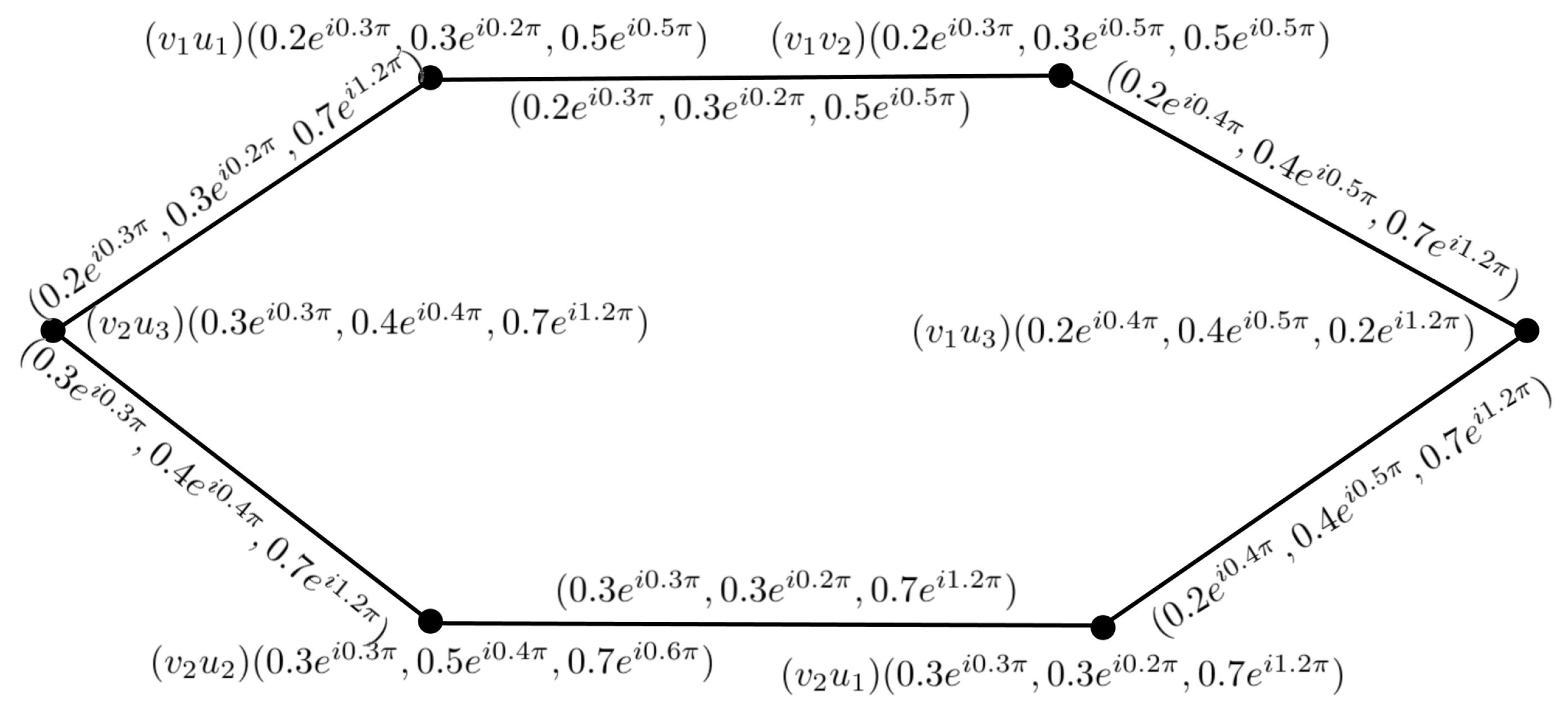
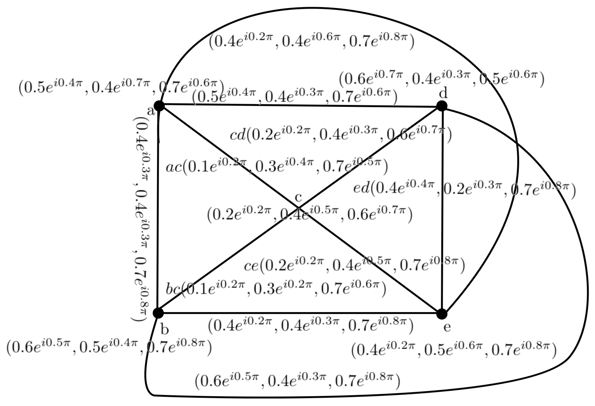
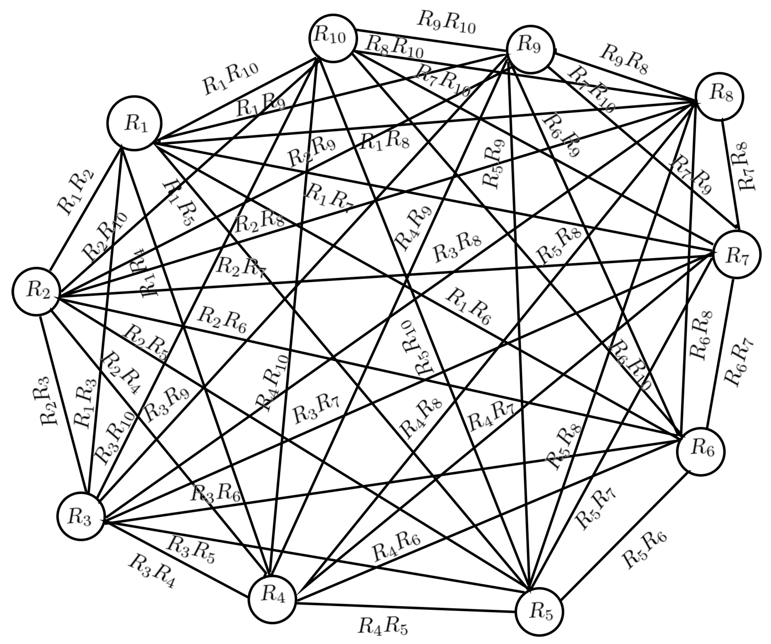
1.

It can be seen from simple calculations that the graph in Figure 1 is a complex neutrosophic graph.

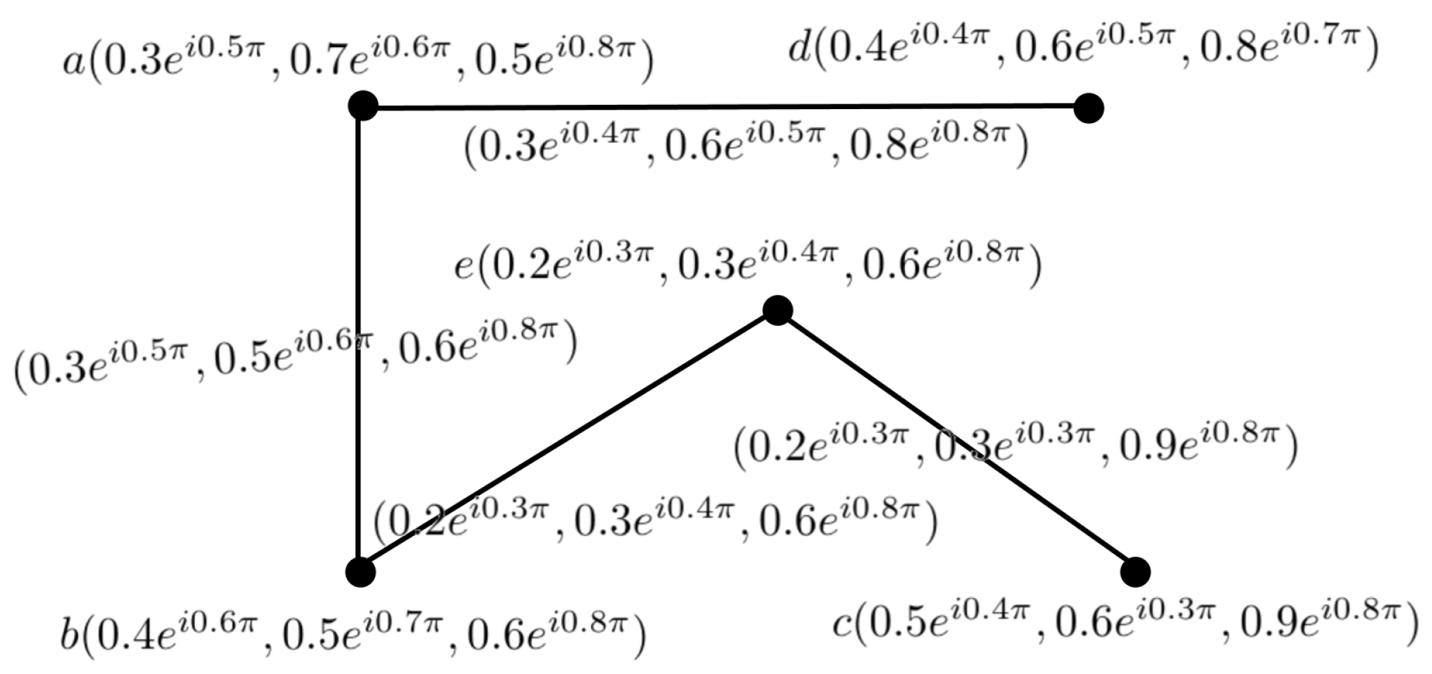
2.

$O\left(G\right)=(2.8e^{i2.4\pi },1.1e^{2.8\pi },1.7e^{1.4\pi })$

3.

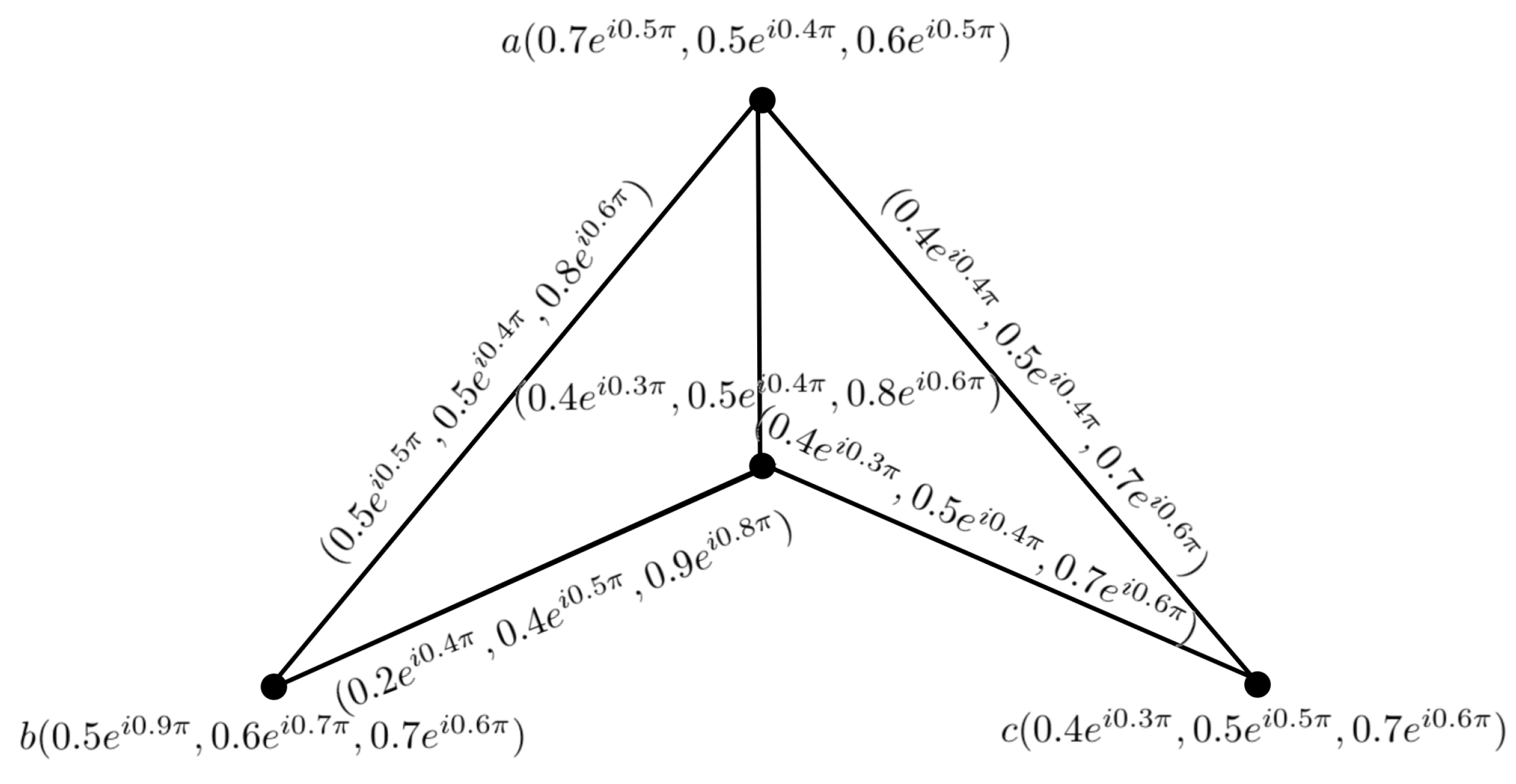
Each vertex in G has a degree of $deg\left(a\right)=0.4,deg\left(b\right)=1.0,deg\left(c\right)=1.8$, and $deg\left(c\right)=0.8$.

Definition 4. 

Let $G=(A,B)$ be a complex neutrosophic graph. The order of a complex neutrosophic graph is defined by

$$O\left(G\right)=(\sum _{\stackrel{`}{w}\in V}{T}^R{\mu }_A\left(\stackrel{`}{w}\right)e^{{\sum }_{\stackrel{`}{w}\in V}i{T}^R{\alpha }_A\left(\stackrel{`}{w}\right)},\sum _{\stackrel{`}{w}\in V}{I}^N{\mu }_A\left(\stackrel{`}{w}\right)e^{{\sum }_{\stackrel{`}{w}\in V}i{I}^D{\beta }_A\left(\stackrel{`}{w}\right)},\sum _{\stackrel{`}{w}\in V}{F}^S{\mu }_B\left(\stackrel{`}{w}\right)e^{{\sum }_{\stackrel{`}{w}\in V}i{F}^S{\gamma }_A\left(\stackrel{`}{w}\right)})$$

and the degree of a vertex $\stackrel{`}{w}$ in G is defined by

$$D\left(G\right)=(\sum _{\stackrel{`}{w}\in E}{T}^R{\mu }_B\left(\stackrel{`}{w}\stackrel{`}{u}\right)e^{{\sum }_{\stackrel{`}{w}\in E}i{T}^R{\alpha }_B\left(\stackrel{`}{w}\stackrel{`}{u}\right)},\sum _{\stackrel{`}{w}\in E}{I}^N{\mu }_B\left(\stackrel{`}{w}\stackrel{`}{u}\right)e^{{\sum }_{\stackrel{`}{w}\in E}i{I}^D{\beta }_B\left(\stackrel{`}{w}\stackrel{`}{u}\right)},\sum _{\stackrel{`}{w}\in E}{F}^S{\mu }_B\left(\stackrel{`}{w}\stackrel{`}{u}\right)e^{{\sum }_{\stackrel{`}{w}\in E}i{F}^S{\gamma }_B\left(\stackrel{`}{w}\stackrel{`}{u}\right)})$$

3. Operations of Complex Neutrosophic Graph

Definition 5. 

Let $G_1=(A_1,B_1)$ and $G_2=(A_2,B_2)$ be two complex neutrosophic graphs; the Cartesian product $G_1\times G_2$ of two complex neutrosophic graphs is defined as a pair $G_1\times G_2=(A_1\times A_2,B_1\times B_2)$, such that

$$\begin{array}{cc}\hfill 1.T^R{\mu }_{A_1\times A_2}({\stackrel{`}{w}}_1,{\stackrel{`}{w}}_2)e^{i{\alpha }_{A_1\times A_2}({\stackrel{`}{w}}_1,{\stackrel{`}{w}}_2)}& =\wedge \{T^R{\mu }_{A_1}\left({\stackrel{`}{w}}_1\right),T^R{\mu }_{A_2}\left({\stackrel{`}{w}}_2\right)\}{e}^{i\wedge \{T^R{\alpha }_{A_1}\left({\stackrel{`}{w}}_1\right),T^R{\alpha }_{A_2}\left({\stackrel{`}{w}}_2\right)\}}\hfill \\ \hfill I^D{\mu }_{A_1\times A_2}({\stackrel{`}{w}}_1,{\stackrel{`}{w}}_2)e^{i{\beta }_{A_1\times A_2}({\stackrel{`}{w}}_1,{\stackrel{`}{w}}_2)}& =\wedge \{I^D{\mu }_{A_1}\left({\stackrel{`}{w}}_1\right),I^D{\mu }_{A_2}\left({\stackrel{`}{w}}_2\right)\}{e}^{i\wedge \{I^D{\beta }_{A_1}\left({\stackrel{`}{w}}_1\right),I^D{\beta }_{A_2}\left({\stackrel{`}{w}}_2\right)\}}\hfill \\ \hfill F^S{\mu }_{A_1\times A_2}({\stackrel{`}{w}}_1,{\stackrel{`}{w}}_2)e^{i{\gamma }_{A_1\times A_2}({\stackrel{`}{w}}_1,{\stackrel{`}{w}}_2)}& =\vee \{F^S{\mu }_{A_1}\left({\stackrel{`}{w}}_1\right),F^S{\mu }_{A_2}\left({\stackrel{`}{w}}_2\right)\}{e}^{i\vee \{F^S{\gamma }_{A_1}\left({\stackrel{`}{w}}_1\right),F^S{\gamma }_{A_2}\left({\stackrel{`}{w}}_2\right)\}}\hfill \end{array}$$

For all ${\stackrel{`}{w}}_1,{\stackrel{`}{w}}_2\in V$.

$$\begin{array}{cc}\hfill 2.T^R{\mu }_{B_1\times B_2}({\stackrel{`}{w}}_1,{\stackrel{`}{w}}_2)e^{i{\alpha }_{B_1\times B_2}({\stackrel{`}{w}}_1,{\stackrel{`}{w}}_2)}& =\wedge \{T^R{\mu }_{B_1}\left({\stackrel{`}{w}}_1\right),T^R{\mu }_{B_2}\left({\stackrel{`}{w}}_2\right)\}{e}^{i\wedge \{T^R{\alpha }_{B_1}\left({\stackrel{`}{w}}_1\right),T^R{\alpha }_{B_2}\left({\stackrel{`}{w}}_2\right)\}}\hfill \\ \hfill I^D{\mu }_{B_1\times B_2}({\stackrel{`}{w}}_1,{\stackrel{`}{w}}_2)e^{i{\beta }_{B_1\times B_2}({\stackrel{`}{w}}_1,{\stackrel{`}{w}}_2)}& =\wedge \{I^D{\mu }_{B_1}\left({\stackrel{`}{w}}_1\right),I^D{\mu }_{B_2}\left({\stackrel{`}{w}}_2\right)\}{e}^{i\wedge \{I^D{\beta }_{B_1}\left({\stackrel{`}{w}}_1\right),I^D{\beta }_{B_2}\left({\stackrel{`}{w}}_2\right)\}}\hfill \\ \hfill F^S{\mu }_{B_1\times B_2}({\stackrel{`}{w}}_1,{\stackrel{`}{w}}_2)e^{i{\gamma }_{B_1\times B_2}({\stackrel{`}{w}}_1,{\stackrel{`}{w}}_2)}& =\vee \{F^S{\mu }_{B_1}\left({\stackrel{`}{w}}_1\right),F^S{\mu }_{B_2}\left({\stackrel{`}{w}}_2\right)\}{e}^{i\vee \{F^S{\gamma }_{B_1}\left({\stackrel{`}{w}}_1\right),F^S{\gamma }_{B_2}\left({\stackrel{`}{w}}_2\right)\}}\hfill \end{array}$$

For all ${\stackrel{`}{w}}_1\in V_1$ and ${\stackrel{`}{w}}_2{\stackrel{`}{u}}_2\in E_2$.

$$\begin{array}{cc}\hfill 3.T^R{\mu }_{B_1\times B_2}(({\stackrel{`}{w}}_1,z),({\stackrel{`}{u}}_1,\stackrel{`}{t}))e^{i{\alpha }_{B_1\times B_2}(({\stackrel{`}{w}}_1,\stackrel{`}{t}),({\stackrel{`}{u}}_1,\stackrel{`}{t}))}& =\wedge \left\{T^R{\mu }_{B_1}(\left({\stackrel{`}{w}}_1{\stackrel{`}{u}}_1\right),T^R{\mu }_{A_2}\left(\stackrel{`}{t}\right))\right\}{e}^{i\wedge \left\{T^R{\alpha }_{B_1}(\left({\stackrel{`}{w}}_1{\stackrel{`}{u}}_1\right),T^R{\alpha }_{A_2}\left(\stackrel{`}{t}\right))\right\}}\hfill \\ \hfill I^D{\mu }_{B_1\times B_2}(({\stackrel{`}{w}}_1,\stackrel{`}{t}),({\stackrel{`}{u}}_1,\stackrel{`}{t}))e^{i{\beta }_{B_1\times B_2}(({\stackrel{`}{w}}_1,\stackrel{`}{t}),({\stackrel{`}{u}}_1,\stackrel{`}{t}))}& =\wedge \left\{I^D{\mu }_{B_1}(\left({\stackrel{`}{w}}_1{\stackrel{`}{u}}_1\right),I^D{\mu }_{A_2}\left(\stackrel{`}{t}\right))\right\}{e}^{i\wedge \left\{I^D{\beta }_{B_1}(\left({\stackrel{`}{w}}_1{\stackrel{`}{u}}_1\right),I^D{\beta }_{A_2}\left(\stackrel{`}{t}\right))\right\}}\hfill \\ \hfill F^S{\mu }_{B_1\times B_2}(({\stackrel{`}{w}}_1,\stackrel{`}{t}),({\stackrel{`}{u}}_1,\stackrel{`}{t}))e^{i{\gamma }_{B_1\times B_2}(({\stackrel{`}{w}}_1,\stackrel{`}{t}),({\stackrel{`}{u}}_1,\stackrel{`}{t}))}& =\vee \{F^S{\mu }_{B_1}(\left({\stackrel{`}{w}}_1{\stackrel{`}{u}}_1\right),F^S{\mu }_{B_2}\left(\left({\stackrel{`}{w}}_1{\stackrel{`}{u}}_1\right)\right\}{e}^{i\vee \left\{F^S{\gamma }_{B_1}(\left({\stackrel{`}{w}}_1{\stackrel{`}{u}}_1\right),F^S{\gamma }_{A_2}\left(\stackrel{`}{t}\right))\right\}}\hfill \end{array}$$

For all $\stackrel{`}{t}\in V_2$ and ${\stackrel{`}{w}}_1{\stackrel{`}{u}}_1\in E_1$.

Definition 6. 

Let $G_1\times G_2$ be two complex neutrosophic graphs. The degree of a vertex in $G_1\times G_2$ can be defined as follows: for any $({\stackrel{`}{w}}_1,{\stackrel{`}{w}}_2)\in V_1\times V_2$,

$$\begin{array}{c}{D}_{G_1\times G_2}({\stackrel{`}{w}}_1,{\stackrel{`}{w}}_2)=\hfill \\ ({\sum }_{({\stackrel{`}{w}}_1,{\stackrel{`}{w}}_2)({\stackrel{`}{u}}_1,{\stackrel{`}{u}}_2)\in E}{T}^R{\mu }_{B_1\times B_2}(({\stackrel{`}{w}}_1,{\stackrel{`}{w}}_2),({\stackrel{`}{u}}_1,{\stackrel{`}{u}}_2))e^{i{\sum }_{({\stackrel{`}{w}}_1,{\stackrel{`}{w}}_2)({\stackrel{`}{u}}_1,{\stackrel{`}{u}}_2)\in E}{T}^R{\alpha }_{B_1\times B_2}(({\stackrel{`}{w}}_1,{\stackrel{`}{w}}_2),({\stackrel{`}{u}}_1,{\stackrel{`}{u}}_2))},\hfill \\ {\sum }_{({\stackrel{`}{w}}_1,{\stackrel{`}{w}}_2)({\stackrel{`}{u}}_1,{\stackrel{`}{u}}_2)\in E}{I}^D{\mu }_{B_1\times B_2}(({\stackrel{`}{w}}_1,{\stackrel{`}{w}}_2),({\stackrel{`}{u}}_1,{\stackrel{`}{u}}_2))e^{i{\sum }_{({\stackrel{`}{w}}_1,{\stackrel{`}{w}}_2)({\stackrel{`}{u}}_1,{\stackrel{`}{u}}_2)\in E}{I}^D{\beta }_{B_1\times B_2}(({\stackrel{`}{w}}_1,{\stackrel{`}{w}}_2),({\stackrel{`}{u}}_1,{\stackrel{`}{u}}_2))},\hfill \\ {\sum }_{({\stackrel{`}{w}}_1,{\stackrel{`}{w}}_2)({\stackrel{`}{u}}_1,{\stackrel{`}{u}}_2)\in E}{F}^S{\mu }_{B_1\times B_2}(({\stackrel{`}{w}}_1,{\stackrel{`}{w}}_2),({\stackrel{`}{u}}_1,{\stackrel{`}{u}}_2))e^{i{\sum }_{({\stackrel{`}{w}}_1,{\stackrel{`}{w}}_2)({\stackrel{`}{u}}_1,{\stackrel{`}{u}}_2)\in E}{F}^S{\gamma }_{B_1\times B_2}(({\stackrel{`}{w}}_1,{\stackrel{`}{w}}_2),({\stackrel{`}{u}}_1,{\stackrel{`}{u}}_2))})\hfill \end{array}$$

Example 2. 

Consider the two complex neutrosophic graphs $G_1$ and $G_2$, as shown in Figure 2 and Figure 3, and their Cartesian product, as shown in Figure 4.

Then, their corresponding Cartesian product $G_1\times G_2$ is shown in Figure 4.

Theorem 1. 

The Cartesian product of two complex neutrosophic graphs is a complex neutrosophic graph.

Proof. 

The conditions for $A_1\times A_2$ are obvious; therefore, we verify only the conditions for $B_1\times B_2$. Let $\stackrel{`}{w}\in V_1$ and ${\stackrel{`}{w}}_2{\stackrel{`}{u}}_2\in E_2$. Then,

$T^R{\mu }_{B_1\times B_2}((\stackrel{`}{w},{\stackrel{`}{w}}_2),(\stackrel{`}{w},{\stackrel{`}{u}}_2))e^{i{\alpha }_{B_1\times B_2}((\stackrel{`}{w},{\stackrel{`}{w}}_2),(\stackrel{`}{w},{\stackrel{`}{u}}_2))}$

$$\begin{array}{ccc}& =& \wedge \{T^R{\mu }_{A_1}\left(\stackrel{`}{w}\right),T^R{\mu }_{B_2}\left({\stackrel{`}{w}}_2{\stackrel{`}{u}}_2\right))\}{e}^{i\wedge \{T^R{\alpha }_{A_1}\left(\stackrel{`}{w}\right),T^R{\alpha }_{B_2}\left({\stackrel{`}{w}}_2{\stackrel{`}{u}}_2\right)\}}\hfill \\ & \le & \wedge \{T^R{\mu }_{A_1}\left(\stackrel{`}{w}\right),\wedge \left\{T^R{\mu }_{B_2}({\stackrel{`}{w}}_2,{\stackrel{`}{u}}_2)\right\}\}{e}^{i\wedge \{T^R{\mu }_{A_1}\left(\stackrel{`}{w}\right),\wedge \{T^R{\mu }_{A_2}\left({\stackrel{`}{w}}_2\right),T^R{\mu }_{A_2}\left({\stackrel{`}{u}}_2\right)\}\}}\hfill \\ & =& \wedge \{\wedge \{T^R{\mu }_{A_1}\left(\stackrel{`}{w}\right),T^R{\mu }_{A_2}\left({\stackrel{`}{w}}_2\right)\},\wedge \{T^R{\mu }_{A_1}\left(\stackrel{`}{w}\right),T^R{\mu }_{A_2}\left({\stackrel{`}{u}}_2\right)\}\},\hfill \\ & & e^{i\wedge \{\wedge \{T^R{\mu }_{A_1}\left(\stackrel{`}{w}\right),T^R{\mu }_{A_2}\left({\stackrel{`}{w}}_2\right)\},\wedge \{T^R{\mu }_{A_1}\left(\stackrel{`}{w}\right),T^R{\mu }_{A_2}\left({\stackrel{`}{u}}_2\right)\}\}}\hfill \\ & =& \wedge \{T^R{\mu }_{A_1\times A_2}((\stackrel{`}{w},{\stackrel{`}{w}}_2),T^R{\mu }_{A_1\times A_2}\left((\stackrel{`}{w},{\stackrel{`}{u}}_2)\right\}{e}^{i\wedge \{T^R{\mu }_{A_1\times A_2}((\stackrel{`}{w},{\stackrel{`}{w}}_2),T^R{\mu }_{A_1\times A_2}\left((\stackrel{`}{w},{\stackrel{`}{u}}_2)\right\}}\hfill \end{array}$$

$I^D{\mu }_{B_1\times B_2}((\stackrel{`}{w},{\stackrel{`}{w}}_2),(\stackrel{`}{w},{\stackrel{`}{u}}_2))e^{i{\beta }_{B_1\times B_2}((\stackrel{`}{w},{\stackrel{`}{w}}_2),(\stackrel{`}{w},{\stackrel{`}{u}}_2))}$

$$\begin{array}{ccc}& =& \wedge \{I^D{\mu }_{A_1}\left(\stackrel{`}{w}\right),I^D{\mu }_{B_2}\left({\stackrel{`}{w}}_2{\stackrel{`}{u}}_2\right))\}{e}^{i\wedge \{I^D{\beta }_{A_1}\left(\stackrel{`}{w}\right),I^D{\beta }_{B_2}\left({\stackrel{`}{w}}_2{\stackrel{`}{u}}_2\right)\}}\hfill \\ & \le & \wedge \{I^D{\mu }_{A_1}\left(\stackrel{`}{w}\right),\wedge \left\{I^D{\mu }_{B_2}({\stackrel{`}{w}}_2,{\stackrel{`}{u}}_2)\right\}\}{e}^{i\wedge \{I^D{\beta }_{A_1}\left(\stackrel{`}{w}\right),\wedge \{I^D{\beta }_{A_2}\left({\stackrel{`}{w}}_2\right),I^D{\beta }_{A_2}\left({\stackrel{`}{u}}_2\right)\}\}}\hfill \\ & =& \wedge \{\wedge \{I^D{\mu }_{A_1}\left(\stackrel{`}{w}\right),I^D{\mu }_{A_2}\left({\stackrel{`}{w}}_2\right)\},\wedge \{I^D{\mu }_{A_1}\left(\stackrel{`}{w}\right),I^D{\mu }_{A_2}\left({\stackrel{`}{u}}_2\right)\}\},\hfill \\ & & e^{i\wedge \{\wedge \{I^D{\beta }_{A_1}\left(\stackrel{`}{w}\right),I^D{\beta }_{A_2}\left({\stackrel{`}{w}}_2\right)\},\wedge \{I^D{\beta }_{A_1}\left(\stackrel{`}{w}\right),I^D{\beta }_{A_2}\left({\stackrel{`}{u}}_2\right)\}\}}\hfill \\ & =& \wedge \{I^D{\mu }_{A_1\times A_2}((\stackrel{`}{w},{\stackrel{`}{w}}_2),I^D{\mu }_{A_1\times A_2}\left((\stackrel{`}{w},{\stackrel{`}{u}}_2)\right\}{e}^{i\wedge \{I^D{\beta }_{A_1\times A_2}((\stackrel{`}{w},{\stackrel{`}{w}}_2),I^D{\beta }_{A_1\times A_2}\left((\stackrel{`}{w},{\stackrel{`}{u}}_2)\right\}}\hfill \end{array}$$

$F^S{\mu }_{B_1\times B_2}((\stackrel{`}{w},{\stackrel{`}{w}}_2),(\stackrel{`}{w},{\stackrel{`}{u}}_2))e^{i{\gamma }_{B_1\times B_2}((\stackrel{`}{w},{\stackrel{`}{w}}_2),(\stackrel{`}{w},{\stackrel{`}{u}}_2))}$

$$\begin{array}{ccc}& =& \vee \{F^S{\mu }_{A_1}\left(\stackrel{`}{w}\right),F^S{\mu }_{B_2}\left(\stackrel{`}{w}2\stackrel{`}{u}2\right))\}{e}^{i\vee \{A^S{\gamma }_{A_1}\left(\stackrel{`}{w}\right),F^S{\gamma }_{B_2}\left(\stackrel{`}{w}2\stackrel{`}{u}2\right)\}}\hfill \\ & \le & \vee \{F^S{\mu }_{A_1}\left(\stackrel{`}{w}\right),\vee \left\{F^S{\mu }_{B_2}(\stackrel{`}{w}2,\stackrel{`}{u}2)\right\}\}{e}^{i\vee \{F^S{\gamma }_{A_1}\left(\stackrel{`}{w}\right),\vee \{T^R{\gamma }_{A_2}\left(\stackrel{`}{w}2\right),T^R\gamma A_2\left({\stackrel{`}{u}}_2\right)\}\}}\hfill \\ & =& \vee \{\vee \{F^S{\mu }_{A_1}\left(\stackrel{`}{w}\right),F^S{\mu }_{A_2}\left(\stackrel{`}{w}2\right)\},\vee \{F^S{\mu }_{A_1}\left(\stackrel{`}{w}\right),F^S{\mu }_{A_2}\left(\stackrel{`}{u}2\right)\}\},\hfill \\ & & e^{i\vee \{\vee \{F^S{\gamma }_{A_1}\left(\stackrel{`}{w}\right),F^S{\gamma }_{A_2}\left(\stackrel{`}{w}2\right)\},\vee \{F^S{\gamma }_{A_1}\left(\stackrel{`}{w}\right),F^S{\gamma }_{A_2}\left({\stackrel{`}{u}}_2\right)\}\}}\hfill \\ & =& \vee \{F^S{\gamma }_{A_1\times A_2}((\stackrel{`}{w},\stackrel{`}{w}2),F^S{\gamma }_{A_1\times A_2}\left((\stackrel{`}{w},\stackrel{`}{u}2)\right\}{e}^{i\vee \{F^S{\gamma }_{A_1\times A_2}((\stackrel{`}{w},\stackrel{`}{w}2),F^S{\gamma }_{A_1\times A_2}\left((\stackrel{`}{w},{\stackrel{`}{u}}_2)\right\}}\hfill \end{array}$$

Similarly, we can prove it for $\stackrel{`}{t}\in V_2$ and ${\stackrel{`}{w}}_1{\stackrel{`}{u}}_1\in E_1.$ □

Definition 7. 

Let $G_1=(A_1,B_1)$ and $G_2=(A_2,B_2)$ be two complex neutrosophic graphs; then, the composition $G_1\circ G_2$ of two complex neutrosophic graphs is defined as a pair $G_1\circ G_2=(A_1\circ A_2,B_1\circ B_2$), such that

$$\begin{array}{c}\hfill 1.T^R{\mu }_{A_1\circ A_2}\left(({\stackrel{`}{w}}_1,{\stackrel{`}{w}}_2)\right)e^{i{T}^R{\alpha }_{A_1\circ A_2}\left(({\stackrel{`}{w}}_1,{\stackrel{`}{w}}_2)\right)}=\wedge \{T^R{\mu }_{A_1}\left({\stackrel{`}{w}}_1\right),T^R{\mu }_{A_1}\left({\stackrel{`}{w}}_2\right)\}{e}^{i\wedge \{T^R{\alpha }_{A_1}\left({\stackrel{`}{w}}_1\right),T^R{\alpha }_{A_2}\left({\stackrel{`}{w}}_2\right)\}}\\ \hfill I^D{\mu }_{A_1\circ A_2}\left(({\stackrel{`}{w}}_1,{\stackrel{`}{w}}_2)\right)e^{i{I}^D\_A_1\circ A_2\left(({\stackrel{`}{w}}_1,{\stackrel{`}{w}}_2)\right)}=\wedge \{I^D{\mu }_{A_1}\left({\stackrel{`}{w}}_1\right),I^D{\mu }_{A_1}\left({\stackrel{`}{w}}_2\right)\}{e}^{i\wedge \{I^D{\beta }_{A_1}\left({\stackrel{`}{w}}_1\right),I^D{\beta }_{A_1}\left({\stackrel{`}{w}}_2\right)\}}\\ \hfill F^S{\mu }_{A_1\circ A_2}\left(({\stackrel{`}{w}}_1,{\stackrel{`}{w}}_2)\right)e^{i{F}^S{\gamma }_{A_1\circ A_2}\left(({\stackrel{`}{w}}_1,{\stackrel{`}{w}}_2)\right)}=\vee \{F^S{\mu }_{A_1}\left({\stackrel{`}{w}}_1\right),F^S{\mu }_{A_1}\left({\stackrel{`}{w}}_2\right)\}{e}^{i\vee \{F^S{\gamma }_{A_1}\left({\stackrel{`}{w}}_1\right),F^S{\gamma }_{A_2}\left({\stackrel{`}{w}}_2\right)\}}\end{array}$$

For all ${\stackrel{`}{w}}_1,{\stackrel{`}{w}}_2\in V$.

$$\begin{array}{c}\hfill 2.T^R{\mu }_{B_1\circ B_2}\left(({\stackrel{`}{w}}_1,{\stackrel{`}{w}}_2)\right)e^{i{T}^R{\alpha }_{B_1\circ B_2}\left(({\stackrel{`}{w}}_1,{\stackrel{`}{w}}_2)\right)}=\wedge \{T^R{\mu }_{B_1}\left({\stackrel{`}{w}}_1\right),T^R{\mu }_{B_1}\left({\stackrel{`}{w}}_2\right)\}{e}^{i\wedge \{T^R{\alpha }_{B_1}\left({\stackrel{`}{w}}_1\right),T^R{\alpha }_{B_2}\left({\stackrel{`}{w}}_2\right)\}}\\ \hfill I^D{\mu }_{B_1\circ B_2}\left(({\stackrel{`}{w}}_1,{\stackrel{`}{w}}_2)\right)e^{i{I}^D{\beta }_{B_1\circ B_2}\left(({\stackrel{`}{w}}_1,{\stackrel{`}{w}}_2)\right)}=\wedge \{I^D{\mu }_{B_1}\left({\stackrel{`}{w}}_1\right),I^D{\mu }_{B_1}\left({\stackrel{`}{w}}_2\right)\}{e}^{i\wedge \{I^D{\beta }_{B_1}\left({\stackrel{`}{w}}_1\right),I^D{\beta }_{B_1}\left({\stackrel{`}{w}}_2\right)\}}\\ \hfill F^S{\mu }_{B_1\circ B_2}\left(({\stackrel{`}{w}}_1,{\stackrel{`}{w}}_2)\right)e^{i{F}^S{\gamma }_{B_1\circ B_2}\left(({\stackrel{`}{w}}_1,{\stackrel{`}{w}}_2)\right)}=\vee \{F^S{\mu }_{B_1}\left({\stackrel{`}{w}}_1\right),F^S{\mu }_{B_1}\left({\stackrel{`}{w}}_2\right)\}{e}^{i\vee \{F^S{\gamma }_{B_1}\left({\stackrel{`}{w}}_1\right),F^S{\gamma }_{B_2}\left({\stackrel{`}{w}}_2\right)\}}\end{array}$$

For all ${\stackrel{`}{w}}_1\in V_1,$ and ${\stackrel{`}{w}}_2{\stackrel{`}{u}}_2\in E_2$.

$$\begin{array}{c}\hfill 3.T^R{\mu }_{B_1\circ B_2}\left(({\stackrel{`}{w}}_1,\stackrel{`}{t})({\stackrel{`}{u}}_1,\stackrel{`}{t})\right)e^{i{T}^R{\alpha }_{B_1\circ B_2}\left(({\stackrel{`}{w}}_1,\stackrel{`}{t})({\stackrel{`}{u}}_1,\stackrel{`}{t})\right)}=\wedge \{T^R{\mu }_{B_1}\left({\stackrel{`}{w}}_1{\stackrel{`}{u}}_1\right),T^R{\mu }_{A_2}\left(\stackrel{`}{t}\right)\}{e}^{i\wedge \{T^R{\alpha }_{B_1}\left({\stackrel{`}{w}}_1{\stackrel{`}{u}}_1\right),T^R{\alpha }_{A_2}\left(\stackrel{`}{t}\right)\}}\\ \hfill I^D{\mu }_{B_1\circ B_2}\left(({\stackrel{`}{w}}_1,\stackrel{`}{t})({\stackrel{`}{u}}_1,\stackrel{`}{t})\right)e^{i{I}^D\_B_1\circ B_2\left(({\stackrel{`}{w}}_1,\stackrel{`}{t})({\stackrel{`}{u}}_1,\stackrel{`}{t})\right)}=\wedge \{I^D{\mu }_{B_1}\left({\stackrel{`}{w}}_1{\stackrel{`}{u}}_1\right),I^D{\mu }_{A_2}\left(\stackrel{`}{t}\right)\}{e}^{i\wedge \{I^D{\beta }_{B_1}\left({\stackrel{`}{w}}_1{\stackrel{`}{u}}_1\right),I^D{\beta }_{A_2}\left(\stackrel{`}{t}\right)\}}\\ \hfill F^S{\mu }_{B_1\circ B_2}\left(({\stackrel{`}{w}}_1,\stackrel{`}{t})({\stackrel{`}{u}}_1,\stackrel{`}{t})\right)e^{i{F}^S{\gamma }_{B_1\circ B_2}\left(({\stackrel{`}{w}}_1,\stackrel{`}{t})({\stackrel{`}{u}}_1,\stackrel{`}{t})\right)}=\vee \{F^S{\mu }_{B_1}\left({\stackrel{`}{w}}_1{\stackrel{`}{u}}_1\right),F^S{\mu }_{A_2}\left(\stackrel{`}{t}\right)\}{e}^{i\vee \{F^S{\gamma }_{B_1}\left({\stackrel{`}{w}}_1{\stackrel{`}{u}}_1\right),F^S{\gamma }_{A_2}\left(\stackrel{`}{t}\right)\}}\end{array}$$

For all $\stackrel{`}{t}\in V_2,$ and ${\stackrel{`}{w}}_1{\stackrel{`}{u}}_1\in E_1$.

$$\begin{array}{ccc}\hfill 4.T^R{\mu }_{B_1\circ B_2}\left(({\stackrel{`}{w}}_1,{\stackrel{`}{w}}_2)({\stackrel{`}{u}}_1,{\stackrel{`}{u}}_2)\right)e^{i{T}^R{\alpha }_{B_1\circ B_2}\left(({\stackrel{`}{w}}_1,{\stackrel{`}{w}}_2)({\stackrel{`}{u}}_1,{\stackrel{`}{u}}_2)\right)}& =& \wedge \{T^R{\mu }_{A_2}\left({\stackrel{`}{w}}_2\right),T^R{\mu }_{A_2}\left({\stackrel{`}{u}}_2\right),T^R{\mu }_{B_1}\left({\stackrel{`}{w}}_1{\stackrel{`}{u}}_1\right)\}\hfill \\ & & e^{i\wedge \{T^R{\alpha }_{A_2}\left({\stackrel{`}{w}}_2\right),T^R{\alpha }_{A_2}{\stackrel{`}{u}}_2),T^R{\alpha }_{B_1}\left({\stackrel{`}{w}}_1{\stackrel{`}{u}}_1\right)\}}\hfill \\ \hfill I^D{\mu }_{B_1\circ B_2}\left(({\stackrel{`}{w}}_1,{\stackrel{`}{w}}_2)({\stackrel{`}{u}}_1,{\stackrel{`}{u}}_2)\right)e^{i{I}^D{\beta }_{B_1\circ B_2}\left(({\stackrel{`}{w}}_1,{\stackrel{`}{w}}_2)({\stackrel{`}{u}}_1,{\stackrel{`}{u}}_2)\right)}& =& \wedge \{I^D{\mu }_{A_2}\left({\stackrel{`}{w}}_2\right),I^D{\mu }_{A_2}\left({\stackrel{`}{u}}_2\right),I^D{\mu }_{B_1}\left({\stackrel{`}{w}}_1{\stackrel{`}{u}}_1\right)\}\hfill \\ & & e^{i\wedge \{I^D{\beta }_{A_2}\left({\stackrel{`}{w}}_2\right),I^D{\beta }_{A_2}{\stackrel{`}{u}}_2),I^D{\beta }_{B_1}\left({\stackrel{`}{w}}_1{\stackrel{`}{u}}_1\right)\}}\hfill \\ \hfill F^S{\mu }_{B_1\circ B_2}\left(({\stackrel{`}{w}}_1,{\stackrel{`}{w}}_2)({\stackrel{`}{u}}_1,{\stackrel{`}{u}}_2)\right)e^{i{F}^S{\gamma }_{B_1\circ B_2}\left(({\stackrel{`}{w}}_1,{\stackrel{`}{w}}_2)({\stackrel{`}{u}}_1,{\stackrel{`}{u}}_2)\right)}& =& \vee \{F^S{\mu }_{A_2}\left({\stackrel{`}{w}}_2\right),F^S{\mu }_{A_2}\left({\stackrel{`}{u}}_2\right),F^S{\mu }_{B_1}\left({\stackrel{`}{w}}_1{\stackrel{`}{u}}_1\right)\}\hfill \\ & & e^{i\vee \{F^S{\gamma }_{A_2}\left({\stackrel{`}{w}}_2\right),F^S{\gamma }_{A_2}{\stackrel{`}{u}}_2),F^S{\gamma }_{B_1}\left({\stackrel{`}{w}}_1{\stackrel{`}{u}}_1\right)\}}\hfill \end{array}$$

For all ${\stackrel{`}{w}}_2,{\stackrel{`}{u}}_2\in V_2,{\stackrel{`}{w}}_2\ne {\stackrel{`}{u}}_2$, and ${\stackrel{`}{w}}_1{\stackrel{`}{u}}_1\in E_1$.

Definition 8. 

Let $G_1=(A_1,B_1)$ and $G_2=(A_2,B_2)$ be two complex neutrosophic graphs; then, the $G_1\circ G_2$ be two complex neutrosophic graphs. The degree of a vertex in $G_1\circ G_2$ can be defined as follows: for any $({\stackrel{`}{w}}_1,{\stackrel{`}{w}}_2)\in V_1\circ V_2$,

$$\begin{array}{c}{D}_{G_1\circ G_2}({\stackrel{`}{w}}_1,{\stackrel{`}{w}}_2)=\hfill \\ ({\sum }_{({\stackrel{`}{w}}_1,{\stackrel{`}{w}}_2)({\stackrel{`}{u}}_1,{\stackrel{`}{u}}_2)\in E}{T}^R{\mu }_{B_1\circ B_2}(({\stackrel{`}{w}}_1,{\stackrel{`}{w}}_2),({\stackrel{`}{u}}_1,{\stackrel{`}{u}}_2))e^{i{\sum }_{({\stackrel{`}{w}}_1,{\stackrel{`}{w}}_2)({\stackrel{`}{u}}_1,{\stackrel{`}{u}}_2)\in E}{T}^R{\alpha }_{B_1\circ B_2}(({\stackrel{`}{w}}_1,{\stackrel{`}{w}}_2),({\stackrel{`}{u}}_1,{\stackrel{`}{u}}_2))},\hfill \\ {\sum }_{({\stackrel{`}{w}}_1,{\stackrel{`}{w}}_2)({\stackrel{`}{u}}_1,{\stackrel{`}{u}}_2)\in E}{I}^D{\mu }_{B_1\circ B_2}(({\stackrel{`}{w}}_1,{\stackrel{`}{w}}_2),({\stackrel{`}{u}}_1,{\stackrel{`}{u}}_2))e^{i{\sum }_{({\stackrel{`}{w}}_1,{\stackrel{`}{w}}_2)({\stackrel{`}{u}}_1,{\stackrel{`}{u}}_2)\in E}{I}^D{\beta }_{B_1\circ B_2}(({\stackrel{`}{w}}_1,{\stackrel{`}{w}}_2),({\stackrel{`}{u}}_1,{\stackrel{`}{u}}_2))},\hfill \\ {\sum }_{({\stackrel{`}{w}}_1,{\stackrel{`}{w}}_2)({\stackrel{`}{u}}_1,{\stackrel{`}{u}}_2)\in E}{F}^S{\mu }_{B_1\circ B_2}(({\stackrel{`}{w}}_1,{\stackrel{`}{w}}_2),({\stackrel{`}{u}}_1,{\stackrel{`}{u}}_2))e^{i{\sum }_{({\stackrel{`}{w}}_1,{\stackrel{`}{w}}_2)({\stackrel{`}{u}}_1,{\stackrel{`}{u}}_2)\in E}{F}^S{\gamma }_{B_1\circ B_2}(({\stackrel{`}{w}}_1,{\stackrel{`}{w}}_2),({\stackrel{`}{u}}_1,{\stackrel{`}{u}}_2))}).\hfill \end{array}$$

Example 3. 

Consider the two complex neutrosophic graphs, as shown in Figure 5, and their composition, as shown in Figure 6.

Then, their composition $G_1\circ G_2$ is shown in Figure 6.

Definition 9. 

Let $G_1=(A_1,B_1)$ and $G_2=(A_2,B_2)$ be two complex neutrosophic graphs; then, the union $G_1\cup G_2=\left(A_1\cup A_2,B_1\cup B_2\right)$ of two complex neutrosophic graphs is defined as follows:

1.

$T^R{\mu }_{A_1\cup A_2}\left(\stackrel{`}{w}\right)e^{{iT}^{R_{{\alpha }_{A_1\cup A_2}}}\left(\stackrel{`}{w}\right)}=T^R{\mu }_{A_1}\left(\stackrel{`}{w}\right)e^{{iT}^{R_{{\alpha }_{A_1}}}\left(\stackrel{`}{w}\right)}$

$I^D{\mu }_{A_1\cup A_2}\left(\stackrel{`}{w}\right)e^{i{I}^D{\beta }_{A_1\cup A_2}\left(\stackrel{`}{w}\right)}=I^D{\mu }_{A_1}\left(\stackrel{`}{w}\right)e^{i{I}^D{\beta }_{A_1}\left(\stackrel{`}{w}\right)}$

$F^S{\mu }_{A_1\cup A_2}\left(\stackrel{`}{w}\right)e^{i{F}^S{\gamma }_{A_1\cup A_2}\left(\stackrel{`}{w}\right)}=F^S{\mu }_{A_1}\left(\stackrel{`}{w}\right)e^{i{F}^S{\gamma }_{A_1}\left(\stackrel{`}{w}\right)}$, for $\stackrel{`}{w}\in V_1$ and $\stackrel{`}{w}\notin V_2$.

2.

$T^R{\mu }_{A_1\cup A_2}\left(\stackrel{`}{w}\right)e^{i{T}^R{\alpha }_{A_1\cup A_2}\left(\stackrel{`}{w}\right)}=T^R{\mu }_{A_2}\left(\stackrel{`}{w}\right)e^{i{T}^R{\alpha }_{A_2}\left(\stackrel{`}{w}\right)}$

$I^D{\mu }_{A_1\cup A_2}\left(\stackrel{`}{w}\right)e^{i{I}^D{\beta }_{A_1\cup A_2}\left(\stackrel{`}{w}\right)}=I^D{\mu }_{A_2}\left(\stackrel{`}{w}\right)e^{i{I}^D{\beta }_{A_2}\left(\stackrel{`}{w}\right)}$

$F^S{\mu }_{A_1\cup A_2}\left(\stackrel{`}{w}\right)e^{i{F}^S{\gamma }_{A_1\cup A_2}\left(\stackrel{`}{w}\right)}=F^S{\mu }_{A_2}\left(\stackrel{`}{w}\right)e^{i{F}^S{\gamma }_{A_2}\left(\stackrel{`}{w}\right)}$, for $\stackrel{`}{w}\in V_2$ and $\stackrel{`}{w}\notin V_1$.

3.

$T^R{\mu }_{A_1\cup A_2}\left(\stackrel{`}{w}\right)e^{i{T}^R{\alpha }_{A_1\cup A_2}\left(\stackrel{`}{w}\right)}=\vee \{T^R{\mu }_{A_2}\left(\stackrel{`}{w}\right),T^R{\mu }_{A_2}\left(\stackrel{`}{w}\right)\}{e}^{i\vee \{T^R{\alpha }_{A_2}\left(\stackrel{`}{w}\right),T^R{\alpha }_{A_2}\left(\stackrel{`}{w}\right)\}}$

$I^D{\mu }_{A_1\cup A_2}\left(\stackrel{`}{w}\right)e^{i{I}^D{\beta }_{A_1\cup A_2}\left(\stackrel{`}{w}\right)}=\vee \{I^D{\mu }_{A_2}\left(\stackrel{`}{w}\right),I^D{\mu }_{A_2}\left(\stackrel{`}{w}\right)\}{e}^{i\vee \{I^D{\beta }_{A_2}\left(\stackrel{`}{w}\right),I^D{\beta }_{A_2}\left(\stackrel{`}{w}\right)\}}$

$F^S{\mu }_{A_1\cup A_2}\left(\stackrel{`}{w}\right)e^{i{F}^S{\gamma }_{A_1\cup A_2}\left(\stackrel{`}{w}\right)}=\wedge \{F^D{\mu }_{A_2}\left(\stackrel{`}{w}\right),F^S{\mu }_{A_2}\left(\stackrel{`}{w}\right)\}{e}^{i\wedge \{F^S{\gamma }_{A_2}\left(\stackrel{`}{w}\right),F^S{\gamma }_{A_2}\left(\stackrel{`}{w}\right)\}}$,

for $\stackrel{`}{w}\in V_1\cap V_2$.

4.

$T^R{\mu }_{B_1\cup B_2}\left(\stackrel{`}{w}\stackrel{`}{u}\right)e^{i{T}^R{\alpha }_{B_1\cup B_2}\left(\stackrel{`}{w}\stackrel{`}{u}\right)}=T^R{\mu }_{B_1}\left(\stackrel{`}{w}\stackrel{`}{u}\right)e^{i{T}^R{\alpha }_{B_1}\left(\stackrel{`}{w}\stackrel{`}{u}\right)}$

$I^D{\mu }_{B_1\cup B_2}\left(\stackrel{`}{w}\stackrel{`}{u}\right)e^{i{I}^D{\beta }_{B_1\cup B_2}\left(\stackrel{`}{w}\stackrel{`}{u}\right)}=I^D{\mu }_{B_1}\left(\stackrel{`}{w}\stackrel{`}{u}\right)e^{i{I}^D{\beta }_{B_1}\left(\stackrel{`}{w}\stackrel{`}{u}\right)}$

$F^S{\mu }_{B_1\cup B_2}\left(\stackrel{`}{w}\stackrel{`}{u}\right)e^{i{F}^S{\gamma }_{B_1\cup B_2}\left(\stackrel{`}{w}\stackrel{`}{u}\right)}=F^S{\gamma }_{B_1}\left(\stackrel{`}{w}\stackrel{`}{u}\right)e^{i{F}^S{\gamma }_{B_1}\left(\stackrel{`}{w}\stackrel{`}{u}\right)}$, for $\stackrel{`}{w}\stackrel{`}{u}\in E_1$ and $\stackrel{`}{w}\stackrel{`}{u}\notin E_2$.

5.

$T^R{\mu }_{B_1\cup B_2}\left(\stackrel{`}{w}\stackrel{`}{u}\right)e^{i{T}^R{\alpha }_{B_1\cup B_2}\left(\stackrel{`}{w}\stackrel{`}{u}\right)}=T^R{\mu }_{B_2}\left(\stackrel{`}{w}\stackrel{`}{u}\right)e^{i{T}^R{\alpha }_{B_2}\left(\stackrel{`}{w}\stackrel{`}{u}\right)}$

$I^D{\mu }_{B_1\cup B_2}\left(\stackrel{`}{w}\stackrel{`}{u}\right)e^{i{I}^D{\beta }_{B_1\cup B_2}\left(\stackrel{`}{w}\stackrel{`}{u}\right)}=I^D{\mu }_{B_2}\left(\stackrel{`}{w}\stackrel{`}{u}\right)e^{i{I}^D{\beta }_{B_2}\left(\stackrel{`}{w}\stackrel{`}{u}\right)}$

$F^S{\mu }_{B_1\cup B_2}\left(\stackrel{`}{w}\stackrel{`}{u}\right)e^{i{F}^S{\gamma }_{B_1\cup B_2}\left(\stackrel{`}{w}\stackrel{`}{u}\right)}=F^S{\mu }_{B_2}\left(\stackrel{`}{w}\stackrel{`}{u}\right)e^{i{F}^S{\gamma }_{B_2}\left(\stackrel{`}{w}\stackrel{`}{u}\right)}$, for $\stackrel{`}{w}\stackrel{`}{u}\in E_2$ and $\stackrel{`}{w}\stackrel{`}{u}\notin E_1$.

6.

$T^R{\mu }_{B_1\cup B_2}\left(\stackrel{`}{w}\stackrel{`}{u}\right)e^{i{T}^R{\alpha }_{B_1\cup B_2}\left(\stackrel{`}{w}\stackrel{`}{u}\right)}=\vee \{T^R{\mu }_{B_2}\left(\stackrel{`}{w}\stackrel{`}{u}\right),T^R{\mu }_{B_2}\left(\stackrel{`}{w}\stackrel{`}{u}\right)\}{e}^{i\vee \{T^R{\alpha }_{B_2}\left(\stackrel{`}{w}\stackrel{`}{u}\right),T^R{\alpha }_{B_2}\left(\stackrel{`}{w}\stackrel{`}{u}\right)\}}$

$I^D{\mu }_{B_1\cup B_2}\left(\stackrel{`}{w}\stackrel{`}{u}\right)e^{i{I}^D{\beta }_{B_1\cup B_2}\left(\stackrel{`}{w}\stackrel{`}{u}\right)}=\vee \{I^D{\mu }_{B_2}\left(\stackrel{`}{w}\stackrel{`}{u}\right),I^D{\mu }_{B_2}\left(\stackrel{`}{w}\stackrel{`}{u}\right)\}{e}^{i\vee \{I^D{\beta }_{B_2}\left(\stackrel{`}{w}\stackrel{`}{u}\right),I^D{\beta }_{B_2}\left(\stackrel{`}{w}\stackrel{`}{u}\right)\}}$

$F^S{\mu }_{B_1\cup B_2}\left(\stackrel{`}{w}\stackrel{`}{u}\right)e^{i{F}^S{\gamma }_{B_1\cup B_2}\left(\stackrel{`}{w}\stackrel{`}{u}\right)}=\wedge \{I^D{\mu }_{B_2}\left(\stackrel{`}{w}\stackrel{`}{u}\right),F^S{\mu }_{B_2}\left(\stackrel{`}{w}\stackrel{`}{u}\right)\}{e}^{i\wedge \{F^S{\gamma }_{B_2}\left(\stackrel{`}{w}\stackrel{`}{u}\right),F^S{\gamma }_{B_2}\left(\stackrel{`}{w}\stackrel{`}{u}\right)\}}$,

for $\stackrel{`}{w}\stackrel{`}{u}\in E_1\cap E_2$.

Example 4. 

Consider the two complex neutrosophic graphs, as shown in Figure 7, and their union, as shown in Figure 8.

Definition 10. 

Let $G_1=(A_1,B_1)$ and $G_2=(A_2,B_2)$ be two complex neutrosophic graphs; then, the join $G_1+G_2=(A_1+A_2,B_1+B_2)$ of the two complex neutrosophic graphs, where $V_1\bigcap V_2=⌀$, is defined as follows:

1.

$T^R{\mu }_{A_1|A_2}\left(\stackrel{`}{w}\right)e^{i{T}^R{\alpha }_{A_1+A_2}\left(\stackrel{`}{w}\right)}=T^R{\mu }_{A_1\cup A_2}\left(\stackrel{`}{w}\right)e^{i{T}^R{\alpha }_{A_1\cup A_2}\left(\stackrel{`}{w}\right)}$

$I^D{\mu }_{A_1|A_2}\left(\stackrel{`}{w}\right)e^{i{I}^D{\beta }_{A_1+A_2}\left(\stackrel{`}{w}\right)}=I^D{\mu }_{A_1\cup A_2}\left(\stackrel{`}{w}\right)e^{i{I}^D{\beta }_{A_1\cup A_2}\left(\stackrel{`}{w}\right)}$

$F^S{\mu }_{A_1+A_2}\left(\stackrel{`}{w}\right)e^{i{F}^S{\gamma }_{A_1+A_2}\left(\stackrel{`}{w}\right)}=F^S{\mu }_{A_1\cup A_2}\left(\stackrel{`}{w}\right)e^{i{F}^S{\gamma }_{A_1\cup A_2}\left(\stackrel{`}{w}\right)}$, if $\stackrel{`}{w}\in V_1\cup V_2$.

2.

$T^R{\mu }_{B_1|B_2}\left(\stackrel{`}{w}\stackrel{`}{u}\right)e^{i{T}^R{\alpha }_{B_1+B_2}\left(\stackrel{`}{w}\right)}=T^R{\mu }_{A_1\cup A_2}\left(\stackrel{`}{w}\stackrel{`}{u}\right)e^{i{T}^R{\alpha }_{A_1\cup A_2}\left(\stackrel{`}{w}\right)}$

$I^D{\mu }_{B_1|B_2}\left(\stackrel{`}{w}\stackrel{`}{u}\right)e^{i{I}^D{\beta }_{B_1+B_2}\left(\stackrel{`}{w}\right)}=I^D{\mu }_{A_1\cup A_2}\left(\stackrel{`}{w}\stackrel{`}{u}\right)e^{i{I}^D{\beta }_{A_1\cup A_2}\left(\stackrel{`}{w}\right)}$

$F^S{\mu }_{B_1+B_2}\left(\stackrel{`}{w}\stackrel{`}{u}\right)e^{i{F}^S{\gamma }_{B_1+B_2}\left(\stackrel{`}{w}\right)}=F^S{\mu }_{A_1\cup A_2}\left(\stackrel{`}{w}\stackrel{`}{u}\right)e^{i{F}^S{\gamma }_{A_1\cup A_2}\left(\stackrel{`}{w}\right)}$, for $\stackrel{`}{w}\stackrel{`}{u}\in E_1\cap E_2$.

3.

$T^R{\mu }_{B_1+B_2}\left(\stackrel{`}{w}\stackrel{`}{u}\right)e^{i{T}^R{\alpha }_{B_1+B_2}\left(\stackrel{`}{w}\stackrel{`}{u}\right)}=\wedge \{T^R{\mu }_{A_1}\left(\stackrel{`}{w}\right),T^R{\mu }_{A_1}\left(\stackrel{`}{u}\right)\}{e}^{i\wedge \{T^R{\alpha }_{A_1}\left(\stackrel{`}{w}\right),T^R{\alpha }_{A_1}\left(\stackrel{`}{u}\right)\}}$

$I^D{\mu }_{B_1+B_2}\left(\stackrel{`}{w}\stackrel{`}{u}\right)e^{i{I}^D{\beta }_{B_1+B_2}\left(\stackrel{`}{w}\stackrel{`}{u}\right)}=\wedge \{I^D{\mu }_{A_1}\left(\stackrel{`}{w}\right),I^D{\mu }_{A_1}\left(\stackrel{`}{u}\right)\}{e}^{i\wedge \{I^D{\beta }_{A_1}\left(\stackrel{`}{w}\right),I^D{\beta }_{A_1}\left(\stackrel{`}{u}\right)\}}$

$F^S{\mu }_{B_1+B_2}\left(\stackrel{`}{w}\stackrel{`}{u}\right)e^{i{F}^S{\gamma }_{B_1+B_2}\left(\stackrel{`}{w}\stackrel{`}{u}\right)}=\vee \{F^S{\mu }_{A_1}\left(\stackrel{`}{w}\right),F^S{\mu }_{A_1}\left(\stackrel{`}{u}\right)\}{e}^{i\vee \{F^S{\gamma }_{A_1}\left(\stackrel{`}{w}\right),F^S{\gamma }_{A_1}\left(\stackrel{`}{u}\right)\}}$.

Here, $\stackrel{`}{w}\stackrel{`}{u}\in E$, where E is the set of all edges joining the vertices of $V_1$ and $V_2$.

Example 5. 

Consider the two complex neutrosophic graphs, as shown in Figure 9, and their join, as shown in Figure 10.

Proposition 1. 

The join of two complex neutrosophic graphs is a neutrosophic graph.

Theorem 2. 

Let $G_1=(A_1,B_1)$ and $G_2=(A_2,B_2)$ be complex neutrosophic graphs of the graphs $G_1^{*}$ and $G_2^{*}$ and let $V_1\cap V_2=⌀$. Then, union $G_1\cup G_2=(A_1\cup A_2,B_1\cup B_2)$ is a complex neutrosophic graph of $G_{*}$ if and only if $G_1$ and $G_2$ are complex neutrosophic graphs of the graphs $G_1^{*}$ and $G_2^{*}$, respectively.

Proof. 

Suppose that $G_1\cup G_2$ is a complex neutrosophic graph. Let $\stackrel{`}{w}\stackrel{`}{u}\notin E_1$ and $\stackrel{`}{w},\stackrel{`}{u}\in V_1-V_2$. Thus,

$$\begin{array}{ccc}\hfill T^R{\mu }_{B_1}\left(\stackrel{`}{w}\stackrel{`}{u}\right)e^{i{T}^R{\alpha }_{B_1}\left(\stackrel{`}{w}\right)}& =& T^R{\mu }_{B_1\cup B_2}\left(\stackrel{`}{w}\stackrel{`}{u}\right)e^{i{T}^R{\alpha }_{B_1\cup B_2}\left(\stackrel{`}{w}\right)}\hfill \\ & =& \wedge \{T^R{\mu }_{A_1\cap A_2}\left(\stackrel{`}{w}\right),T^R{\mu }_{A_1\cap A_2}\left(\stackrel{`}{u}\right)\}{e}^{i\wedge \{T^R{\alpha }_{A_1\cap A_2}\left(\stackrel{`}{w}\right),T^R{\alpha }_{A_1\cap A_2}\left(\stackrel{`}{u}\right)\}}\hfill \\ & =& \wedge \{T^R{\mu }_{A_1}\left(\stackrel{`}{w}\right),T^R{\mu }_{A_1}\left(\stackrel{`}{u}\right)\}{e}^{i\wedge \{T^R{\alpha }_{A_1}\left(\stackrel{`}{w}\right),T^R{\alpha }_{A_1}\left(\stackrel{`}{u}\right)\}}\hfill \\ \hfill I^D{\mu }_{B_1}\left(\stackrel{`}{w}\stackrel{`}{u}\right)e^{i{I}^D{\beta }_{B_1}\left(\stackrel{`}{w}\right)}& =& I^D{\mu }_{B_1\cup B_2}\left(\stackrel{`}{w}\stackrel{`}{u}\right)e^{i{I}^D{\beta }_{B_1\cup B_2}\left(\stackrel{`}{w}\right)}\hfill \\ & =& \wedge \{I^D{\mu }_{A_1\cap A_2}\left(\stackrel{`}{w}\right),I^D{\mu }_{A_1\cap A_2}\left(\stackrel{`}{u}\right)\}{e}^{i\wedge \{I^D{\beta }_{A_1\cap A_2}\left(\stackrel{`}{w}\right),I^D{\alpha }_{A_1\cap A_2}\left(\stackrel{`}{u}\right)\}}\hfill \\ & =& \wedge \{I^D{\mu }_{A_1}\left(\stackrel{`}{w}\right),I^D{\mu }_{A_1}\left(\stackrel{`}{u}\right)\}{e}^{i\wedge \{I^D{\beta }_{A_1}\left(\stackrel{`}{w}\right),I^D{\beta }_{A_1}\left(\stackrel{`}{u}\right)\}}\hfill \\ \hfill F^S{\mu }_{B_1}\left(\stackrel{`}{w}\stackrel{`}{u}\right)e^{i{F}^S{\gamma }_{B_1}\left(\stackrel{`}{w}\right)}& =& F^S{\mu }_{B_1\cup B_2}\left(\stackrel{`}{w}\stackrel{`}{u}\right)e^{i{F}^S{\gamma }_{B_1\cup B_2}\left(\stackrel{`}{w}\right)}\hfill \\ & =& \vee \{F^S{\mu }_{A_1\cap A_2}\left(\stackrel{`}{w}\right),F^S{\mu }_{A_1\cap A_2}\left(\stackrel{`}{u}\right)\}{e}^{i\vee \{F^S{\gamma }_{A_1\cap A_2}\left(\stackrel{`}{w}\right),F^S{\gamma }_{A_1\cap A_2}\left(\stackrel{`}{u}\right)\}}\hfill \\ & =& \vee \{F^S{\gamma }_{A_1}\left(\stackrel{`}{w}\right),F^S{\gamma }_{A_1}\left(\stackrel{`}{u}\right)\}{e}^{i\vee \{F^S{\gamma }_{A_1}\left(\stackrel{`}{w}\right),F^S{\gamma }_{A_1}\left(\stackrel{`}{u}\right)\}}\hfill \end{array}$$

This shows that $G_1=(A_1,B_1)$ is a complex neutrosophic graph. Similarly, we can show that $G_2=(A_2,B_2)$ is a complex neutrosophic graph. The converse part is obvious. □

Theorem 3. 

Let $G_1=(A_1,B_1)$ and $G_2=(A_2,B_2)$ be complex neutrosophic graphs of the graphs $G_1^{*}$ and $G_2^{*}$, and let $V_1\cap V_2=⌀$. Then, join $G_1+G_2=(A_1+A_2,B_1+B_2)$ is a complex neutrosophic graph of $G_{*}$ if and only if $G_1$ and $G_2$ are complex neutrosophic graphs of the graphs $G_1^{*}$ and $G_2^{*}$, respectively.

4. Isomorphism of Complex Neutrosophic Graphs

Definition 11. 

Let $G_1=(A_1,B_1)$ and $G_2=(A_2,B_2)$ be two complex neutrosophic graphs. A homomorphism $g:G_1\to G_2$ is a mapping $g:V_1\to V_2$ such that:

$$1.\left\{\begin{array}{c}{T}^R{\mu }_{A_1}\left({\stackrel{`}{w}}_1\right)e^{i{T}^R{\alpha }_{A_1}\left({\stackrel{`}{w}}_1\right)}\le T^R{\mu }_{A_2}\left(\phi \left({\stackrel{`}{w}}_1\right)\right)e^{i{T}^R{\alpha }_{A_2}\left(\phi \left({\stackrel{`}{w}}_1\right)\right)}\hfill \\ I^D{\mu }_{A_1}\left({\stackrel{`}{w}}_1\right)e^{i{I}^D{\beta }_{A_1}\left({\stackrel{`}{w}}_1\right)}\le I^D{\mu }_{A_2}\left(\phi \left({\stackrel{`}{w}}_1\right)\right)e^{i{I}^D{\beta }_{A_2}\left(\phi \left({\stackrel{`}{w}}_1\right)\right)}forall{\stackrel{`}{w}}_1{\stackrel{`}{u}}_1\in V_1\hfill \\ F^S{\mu }_{A_1}\left({\stackrel{`}{w}}_1\right)e^{i{F}^S{\gamma }_{A_1}\left({\stackrel{`}{w}}_1\right)}\ge F^S{\mu }_{A_2}\left(\phi \left({\stackrel{`}{w}}_1\right)\right)e^{i{F}^S{\gamma }_{A_2}\left(\phi \left({\stackrel{`}{w}}_1\right)\right)}\hfill \end{array}\right.$$

$$2.\left\{\begin{array}{c}{T}^R{\mu }_{B_1}\left({\stackrel{`}{w}}_1{\stackrel{`}{u}}_1\right)e^{i{T}^R{\alpha }_{B_1}\left({\stackrel{`}{w}}_1{\stackrel{`}{u}}_1\right)}\le T^R{\mu }_{B_2}\left(\phi \left({\stackrel{`}{w}}_1\right)\phi \left({\stackrel{`}{u}}_1\right)\right)e^{i{T}^R{\alpha }_{B_2}\left(\phi \left({\stackrel{`}{w}}_1\right)\phi \left({\stackrel{`}{u}}_1\right)\right)}\hfill \\ I^D{\mu }_{B_1}\left({\stackrel{`}{w}}_1{\stackrel{`}{u}}_1\right)e^{i{I}^D{\beta }_{B_1}\left({\stackrel{`}{w}}_1{\stackrel{`}{u}}_1\right)}\le I^D{\mu }_{B_2}\left(\phi \left({\stackrel{`}{w}}_1\right)\phi \left({\stackrel{`}{u}}_1\right)\right)e^{i{I}^D{\beta }_{B_2}\left(\phi \left({\stackrel{`}{w}}_1\right)\phi \left({\stackrel{`}{u}}_1\right)\right)}forall{\stackrel{`}{w}}_1{\stackrel{`}{u}}_1\in E_1\hfill \\ F^S{\mu }_{B_1}\left({\stackrel{`}{w}}_1{\stackrel{`}{u}}_1\right)e^{i{I}^D{\gamma }_{B_1}\left({\stackrel{`}{w}}_1{\stackrel{`}{u}}_1\right)}\ge F^S{\mu }_{B_2}\left(\phi \left({\stackrel{`}{w}}_1\right)\phi \left({\stackrel{`}{u}}_1\right)\right)e^{i{F}^S{\gamma }_{B_2}\left(\phi \left({\stackrel{`}{w}}_1\right)\phi \left({\stackrel{`}{u}}_1\right)\right)}\hfill \end{array}\right.$$

A bijective homomorphism with the property

$$3.\left\{\begin{array}{c}{T}^R{\mu }_{A_1}\left({\stackrel{`}{w}}_1\right)e^{i{T}^R{\alpha }_{A_1}\left({\stackrel{`}{w}}_1\right)}=T^R{\mu }_{A_2}\left(\phi \left({\stackrel{`}{w}}_1\right)\right)e^{i{T}^R{\alpha }_{A_2}\left(\phi \left({\stackrel{`}{w}}_1\right)\right)}\hfill \\ I^D{\mu }_{A_1}\left({\stackrel{`}{w}}_1\right)e^{i{I}^D{\beta }_{A_1}\left({\stackrel{`}{w}}_1\right)}=I^D{\mu }_{A_2}\left(\phi \left({\stackrel{`}{w}}_1\right)\right)e^{i{I}^D{\beta }_{A_2}\left(\phi \left({\stackrel{`}{w}}_1\right)\right)}forall{\stackrel{`}{w}}_1\in V_1\hfill \\ F^S{\mu }_{A_1}\left({\stackrel{`}{w}}_1\right)e^{i{F}^S{\gamma }_{A_1}\left({\stackrel{`}{w}}_1\right)}=F^S{\mu }_{A_2}\left(\phi \left({\stackrel{`}{w}}_1\right)\right)e^{i{F}^S{\gamma }_{A_2}\left(\phi \left({\stackrel{`}{w}}_1\right)\right)}\hfill \end{array}\right.$$

is called a week isomorphism. A bijective homomorphism with the property

$$4.\left\{\begin{array}{c}{T}^R{\mu }_{B_1}\left({\stackrel{`}{w}}_1{\stackrel{`}{u}}_1\right)e^{i{T}^R{\alpha }_{B_1}\left({\stackrel{`}{w}}_1{\stackrel{`}{u}}_1\right)}=T^R{\mu }_{B_2}\left(\phi \left({\stackrel{`}{w}}_1\right)\phi \left({\stackrel{`}{u}}_1\right)\right)e^{i{T}^R{\alpha }_{B_2}\left(\phi \left({\stackrel{`}{w}}_1\right)\phi \left({\stackrel{`}{u}}_1\right)\right)}\hfill \\ I^D{\mu }_{B_1}\left({\stackrel{`}{w}}_1{\stackrel{`}{u}}_1\right)e^{i{I}^D{\beta }_{B_1}\left({\stackrel{`}{w}}_1{\stackrel{`}{u}}_1\right)}=I^D{\mu }_{B_2}\left(\phi \left({\stackrel{`}{w}}_1\right)\phi \left({\stackrel{`}{u}}_1\right)\right)e^{i{I}^D{\beta }_{B_2}\left(\phi \left({\stackrel{`}{w}}_1\right)\phi \left({\stackrel{`}{u}}_1\right)\right)}forall{\stackrel{`}{w}}_1{\stackrel{`}{u}}_1\in E_1\hfill \\ F^S{\mu }_{B_1}\left({\stackrel{`}{w}}_1{\stackrel{`}{u}}_1\right)e^{i{I}^D{\gamma }_{B_1}\left({\stackrel{`}{w}}_1{\stackrel{`}{u}}_1\right)}=F^S{\mu }_{B_2}\left(\phi \left({\stackrel{`}{w}}_1\right)\phi \left({\stackrel{`}{u}}_1\right)\right)e^{i{F}^S{\gamma }_{B_2}\left(\phi \left({\stackrel{`}{w}}_1\right)\phi \left({\stackrel{`}{u}}_1\right)\right)}\hfill \end{array}\right.$$

is called a strong co-isomorphism. A bijective mapping $\phi :G_1\to G_2$ satisfying 3 and 4 is called an isomorphism.

Theorem 4. 

An isomorphism between complex neutrosophic graphs is an equivalence relation.

Proof. 

The reflexivity and symmetry are obvious. To prove the transitivity, we let $\psi :V_1\to V_2$ and $\phi :V_2\to V_3$ be the isomorphism of $G_1$ onto $G_2$ and $G_2$ onto $G_3$, respectively. Then, $\phi \circ \psi :V_1\to V_3$ is a bijective map from $V_1$ to $V_3$, where $(\phi \circ \psi )\left({\stackrel{`}{w}}_1\right)=\phi \left(\psi \left({\stackrel{`}{w}}_1\right)\right)$ for all ${\stackrel{`}{w}}_1\in V_1$. Since a map $\psi :V_1\to V_2$ defined by $\psi \left({\stackrel{`}{w}}_1\right)={\stackrel{`}{w}}_2$ for ${\stackrel{`}{w}}_1\in V_1$ is an isomorphism, here,

$$\begin{array}{}& \hfill T^R{\mu }_{A_1}\left({\stackrel{`}{w}}_1\right)e^{i{T}^R{\alpha }_{A_1}\left({\stackrel{`}{w}}_1\right)}& =T^R{\mu }_{A_2}\left(\psi \left({\stackrel{`}{w}}_1\right)\right)e^{i{T}^R{\alpha }_{A_2}\left(\psi \left({\stackrel{`}{w}}_1\right)\right)}\hfill \hfill \mathrm{(1)}& & =T^R{\mu }_{A_2}\left({\stackrel{`}{w}}_2\right)e^{i{T}^R{\alpha }_{A_2}\left({\stackrel{`}{w}}_2\right)},forall{\stackrel{`}{w}}_1\in V_1\hfill & I^D{\mu }_{A_1}\left({\stackrel{`}{w}}_1\right)e^{i{I}^D{\beta }_{A_1}\left({\stackrel{`}{w}}_1\right)}\hfill & =I^D{\mu }_{A_2}\left(\psi \left({\stackrel{`}{w}}_1\right)\right)e^{i{I}^D{\beta }_{A_2}\left(\psi \left({\stackrel{`}{w}}_1\right)\right)}\hfill \hfill \mathrm{(2)}& & =I^D{\mu }_{A_2}\left({\stackrel{`}{w}}_2\right)e^{i{I}^D{\beta }_{A_2}\left({\stackrel{`}{w}}_2\right)},forall{\stackrel{`}{w}}_1\in V_1\hfill & F^S{\mu }_{A_1}\left({\stackrel{`}{w}}_1\right)e^{i{F}^S{\gamma }_{A_1}\left({\stackrel{`}{w}}_1\right)}\hfill & =F^S{\mu }_{A_2}\left(\phi \left({\stackrel{`}{w}}_1\right)\right)e^{i{F}^S{\gamma }_{A_2}\left(\phi \left({\stackrel{`}{w}}_1\right)\right)}\hfill \hfill \mathrm{(3)}& & =F^S{\mu }_{A_2}\left({\stackrel{`}{w}}_2\right)e^{i{F}^S{\gamma }_{A_2}\left({\stackrel{`}{w}}_2\right)},forall{\stackrel{`}{w}}_1\in V_1\hfill & T^R{\mu }_{B_1}\left({\stackrel{`}{w}}_1{\stackrel{`}{u}}_1\right)e^{i{T}^R{\alpha }_{B_1}\left({\stackrel{`}{w}}_1{\stackrel{`}{u}}_1\right)}\hfill & =T^R{\mu }_{B_2}\left(\psi \left({\stackrel{`}{w}}_1\right)\psi \left({\stackrel{`}{u}}_1\right)\right)e^{i{T}^R{\alpha }_{B_2}\left(\psi \left({\stackrel{`}{w}}_1\right)\psi \left({\stackrel{`}{u}}_1\right)\right)}\hfill \hfill \mathrm{(4)}& & =T^R{\mu }_{B_2}\left({\stackrel{`}{w}}_2{\stackrel{`}{u}}_2\right)e^{i{T}^R{\alpha }_{B_2}\left({\stackrel{`}{w}}_2{\stackrel{`}{u}}_2\right)},forall{\stackrel{`}{w}}_1{\stackrel{`}{u}}_1\in E_1\hfill & I^D{\mu }_{B_1}\left({\stackrel{`}{w}}_1{\stackrel{`}{u}}_1\right)e^{i{I}^D{\beta }_{B_1}\left({\stackrel{`}{w}}_1{\stackrel{`}{u}}_1\right)}\hfill & =I^D{\mu }_{B_2}\left(\psi \left({\stackrel{`}{w}}_1\right)\psi \left({\stackrel{`}{u}}_1\right)\right)e^{i{I}^D{\beta }_{B_2}\left(\psi \left({\stackrel{`}{w}}_1\right)\psi \left({\stackrel{`}{u}}_1\right)\right)}\hfill \hfill \mathrm{(5)}& & =I^D{\mu }_{B_2}\left({\stackrel{`}{w}}_2{\stackrel{`}{u}}_2\right)e^{i{I}^D{\beta }_{B_2}\left({\stackrel{`}{w}}_2{\stackrel{`}{u}}_2\right)},forall{\stackrel{`}{w}}_1{\stackrel{`}{u}}_1\in E_1\hfill & F^S{\mu }_{B_1}\left({\stackrel{`}{w}}_1{\stackrel{`}{u}}_1\right)e^{i{F}^S{\gamma }_{B_1}\left({\stackrel{`}{w}}_1{\stackrel{`}{u}}_1\right)}\hfill & =F^S{\mu }_{B_2}\left(\psi \left({\stackrel{`}{w}}_1\right)\psi \left({\stackrel{`}{u}}_1\right)\right)e^{i{F}^S{\gamma }_{B_2}\left(\psi \left({\stackrel{`}{w}}_1\right)\psi \left({\stackrel{`}{u}}_1\right)\right)}\hfill \hfill \mathrm{(6)}& & =F^S{\mu }_{B_2}\left({\stackrel{`}{w}}_2{\stackrel{`}{u}}_2\right)e^{i{F}^S{\gamma }_{B_2}\left({\stackrel{`}{w}}_2{\stackrel{`}{u}}_2\right)},forall{\stackrel{`}{w}}_1{\stackrel{`}{u}}_1\in E_1.\hfill \end{array}$$

Since a map $\phi :V_2\to V_3$ defined by $\phi \left({\stackrel{`}{w}}_2\right)={\stackrel{`}{w}}_3$ for ${\stackrel{`}{w}}_2\in V_2$ is an isomorphism,

$$\begin{array}{}& \hfill T^R{\mu }_{A_2}\left({\stackrel{`}{w}}_2\right)e^{i{T}^R{\alpha }_{A_2}\left({\stackrel{`}{w}}_2\right)}& =T^R{\mu }_{A_3}\left(\psi \left({\stackrel{`}{w}}_2\right)\right)e^{i{T}^R{\alpha }_{A_3}\left(\psi \left({\stackrel{`}{w}}_2\right)\right)}\hfill \hfill \mathrm{(7)}& & =T^R{\mu }_{A_3}\left({\stackrel{`}{w}}_3\right)e^{i{T}^R{\alpha }_{A_3}\left({\stackrel{`}{w}}_3\right)},forall{\stackrel{`}{w}}_2\in V_1\hfill & \hfill I^D{\mu }_{A_2}\left({\stackrel{`}{w}}_2\right)e^{i{I}^D{\beta }_{A_2}\left({\stackrel{`}{w}}_2\right)}& =I^D{\mu }_{A_3}\left(\psi \left({\stackrel{`}{w}}_2\right)\right)e^{i{I}^D{\beta }_{A_3}\left(\psi \left({\stackrel{`}{w}}_2\right)\right)}\hfill \hfill \mathrm{(8)}& & =I^D{\mu }_{A_3}\left({\stackrel{`}{w}}_3\right)e^{i{I}^D{\beta }_{A_3}\left({\stackrel{`}{w}}_3\right)},forall{\stackrel{`}{w}}_2\in V_1\hfill & \hfill F^S{\mu }_{A_2}\left({\stackrel{`}{w}}_2\right)e^{i{F}^S{\gamma }_{A_2}\left({\stackrel{`}{w}}_2\right)}& =F^S{\mu }_{A_3}\left(\phi \left({\stackrel{`}{w}}_2\right)\right)e^{i{F}^S{\gamma }_{A_3}\left(\phi \left({\stackrel{`}{w}}_2\right)\right)}\hfill \hfill \mathrm{(9)}& & =F^S{\mu }_{A_3}\left({\stackrel{`}{w}}_3\right)e^{i{F}^S{\gamma }_{A_3}\left({\stackrel{`}{w}}_3\right)},forall{\stackrel{`}{w}}_2\in V_1\hfill & \hfill T^R{\mu }_{B_2}\left({\stackrel{`}{w}}_2{\stackrel{`}{u}}_2\right)e^{i{T}^R{\alpha }_{B_2}\left({\stackrel{`}{w}}_2{\stackrel{`}{u}}_2\right)}& =T^R{\mu }_{B_3}\left(\psi \left({\stackrel{`}{w}}_2\right)\psi \left({\stackrel{`}{u}}_2\right)\right)e^{i{T}^R{\alpha }_{B_3}\left(\psi \left({\stackrel{`}{w}}_2\right)\psi \left({\stackrel{`}{u}}_2\right)\right)}\hfill \hfill \mathrm{(10)}& & =T^R{\mu }_{B_3}\left({\stackrel{`}{w}}_3{\stackrel{`}{u}}_3\right)e^{i{T}^R{\alpha }_{B_3}\left({\stackrel{`}{w}}_3{\stackrel{`}{u}}_3\right)},forall{\stackrel{`}{w}}_2{\stackrel{`}{u}}_2\in E_1\hfill & \hfill I^D{\mu }_{B_2}\left({\stackrel{`}{w}}_2{\stackrel{`}{u}}_2\right)e^{i{I}^D{\beta }_{B_2}\left({\stackrel{`}{w}}_2{\stackrel{`}{u}}_2\right)}& =I^D{\mu }_{B_3}\left(\psi \left({\stackrel{`}{w}}_2\right)\psi \left({\stackrel{`}{u}}_2\right)\right)e^{i{I}^D{\beta }_{B_3}\left(\psi \left({\stackrel{`}{w}}_2\right)\psi \left({\stackrel{`}{u}}_2\right)\right)}\hfill \hfill \mathrm{(11)}& & =I^D{\mu }_{B_3}\left({\stackrel{`}{w}}_3{\stackrel{`}{u}}_3\right)e^{i{I}^D{\beta }_{B_3}\left({\stackrel{`}{w}}_3{\stackrel{`}{u}}_3\right)},forall{\stackrel{`}{w}}_2{\stackrel{`}{u}}_2\in E_1\hfill & \hfill F^S{\mu }_{B_2}\left({\stackrel{`}{w}}_2{\stackrel{`}{u}}_2\right)e^{i{F}^S{\gamma }_{B_2}\left({\stackrel{`}{w}}_2{\stackrel{`}{u}}_2\right)}& =F^S{\mu }_{B_3}(\phi \left({\stackrel{`}{w}}_2\phi \left({\stackrel{`}{u}}_2\right)\right)e^{i{F}^S{\gamma }_{B_3}\left(\phi \left({\stackrel{`}{w}}_2\right)\phi \left({\stackrel{`}{u}}_2\right)\right)}\hfill \hfill \mathrm{(12)}& & =F^S{\mu }_{B_3}\left({\stackrel{`}{w}}_3{\stackrel{`}{u}}_3\right)e^{i{F}^S{\gamma }_{B_3}\left({\stackrel{`}{w}}_3{\stackrel{`}{u}}_3\right)},forall{\stackrel{`}{w}}_2{\stackrel{`}{u}}_2\in E_1.\hfill \end{array}$$

From (1), (7), and $\psi \left({\stackrel{`}{w}}_1\right)={\stackrel{`}{w}}_2,{\stackrel{`}{w}}_1\in V_1$, we have

$$\begin{array}{cc}\hfill T^R{\mu }_{A_1}\left({\stackrel{`}{w}}_1\right)e^{i{T}^R{\alpha }_{A_1}\left({\stackrel{`}{w}}_1\right)}& =T^R{\mu }_{A_2}\left(\psi \left({\stackrel{`}{w}}_1\right)\right)e^{i{T}^R{\alpha }_{A_2}\left(\psi \left({\stackrel{`}{w}}_1\right)\right)}\hfill \\ \hfill & =T^R{\mu }_{A_2}\left({\stackrel{`}{w}}_2\right)e^{i{T}^R{\alpha }_{A_2}\left({\stackrel{`}{w}}_2\right)}\hfill \\ \hfill & =T^R{\mu }_{A_2}\left(\phi \left({\stackrel{`}{w}}_2\right)\right)e^{i{T}^R{\alpha }_{A_3}\left(\phi \left({\stackrel{`}{w}}_2\right)\right)}\hfill \\ \hfill & =T^R{\mu }_{A_2}\left(\phi \left(\psi \left({\stackrel{`}{w}}_1\right)\right)\right)e^{i{T}^R{\alpha }_{A_3}\left(\phi \left(\psi \left({\stackrel{`}{w}}_2\right)\right)\right)}.\hfill \end{array}$$

From (2), (8), and $\psi \left({\stackrel{`}{w}}_1\right)={\stackrel{`}{w}}_2,{\stackrel{`}{w}}_1\in V_1$, we have

$$\begin{array}{cc}\hfill I^D{\mu }_{A_1}\left({\stackrel{`}{w}}_1\right)e^{i{I}^D{\beta }_{A_1}\left({\stackrel{`}{w}}_1\right)}& =I^D{\mu }_{A_2}\left(\psi \left({\stackrel{`}{w}}_1\right)\right)e^{i{I}^D{\beta }_{A_2}\left(\psi \left({\stackrel{`}{w}}_1\right)\right)}\hfill \\ \hfill & =I^D{\mu }_{A_2}\left({\stackrel{`}{w}}_2\right)e^{i{I}^D{\beta }_{A_2}\left({\stackrel{`}{w}}_2\right)}\hfill \\ \hfill & =I^D{\mu }_{A_2}\left(\phi \left({\stackrel{`}{w}}_2\right)\right)e^{i{I}^D{\beta }_{A_3}\left(\phi \left({\stackrel{`}{w}}_2\right)\right)}\hfill \\ \hfill & =I^D{\mu }_{A_2}\left(\phi \left(\psi \left({\stackrel{`}{w}}_1\right)\right)\right)e^{i{I}^D{\beta }_{A_3}\left(\phi \left(\psi \left({\stackrel{`}{w}}_2\right)\right)\right)}.\hfill \end{array}$$

From (3), (9), and $\psi \left({\stackrel{`}{w}}_1\right)={\stackrel{`}{w}}_2,{\stackrel{`}{w}}_1\in V_1$, we have

$$\begin{array}{cc}\hfill F^S{\mu }_{A_1}\left({\stackrel{`}{w}}_1\right)e^{i{F}^S{\gamma }_{A_1}\left({\stackrel{`}{w}}_1\right)}& =F^S{\mu }_{A_2}\left(\psi \left({\stackrel{`}{w}}_1\right)\right)e^{i{F}^S{\gamma }_{A_2}\left(\psi \left({\stackrel{`}{w}}_1\right)\right)}\hfill \\ \hfill & =F^S{\mu }_{A_2}\left({\stackrel{`}{w}}_2\right)e^{i{F}^S{\gamma }_{A_2}\left({\stackrel{`}{w}}_2\right)}\hfill \\ \hfill & =F^S{\mu }_{A_2}\left(\phi \left({\stackrel{`}{w}}_2\right)\right)e^{i{F}^S{\gamma }_{A_3}\left(\phi \left({\stackrel{`}{w}}_2\right)\right)}\hfill \\ \hfill & =F^S{\mu }_{A_2}\left(\phi \left(\psi \left({\stackrel{`}{w}}_1\right)\right)\right)e^{i{F}^S{\gamma }_{A_3}\left(\phi \left(\psi \left({\stackrel{`}{w}}_2\right)\right)\right)}.\hfill \end{array}$$

From (4) and (10), we have

$$\begin{array}{cc}\hfill T^R{\mu }_{B_1}\left({\stackrel{`}{w}}_1{\stackrel{`}{u}}_1\right)e^{i{T}^R{\alpha }_{B_1}\left({\stackrel{`}{w}}_1{\stackrel{`}{u}}_1\right)}& =T^R{\mu }_{B_2}\left(\psi \left({\stackrel{`}{w}}_1\right)\psi \left({\stackrel{`}{u}}_1\right)\right)e^{i{T}^R{\alpha }_{B_2}\left(\psi \left({\stackrel{`}{w}}_1\right)\psi \left({\stackrel{`}{u}}_1\right)\right)}\hfill \\ \hfill & =T^R{\mu }_{B_2}\left({\stackrel{`}{w}}_2{\stackrel{`}{u}}_2\right)e^{i{T}^R{\alpha }_{B_2}\left({\stackrel{`}{w}}_2{\stackrel{`}{u}}_2\right)}\hfill \\ \hfill & =T^R{\mu }_{B_3}\left(\phi \left({\stackrel{`}{w}}_2\right)\phi \left({\stackrel{`}{u}}_2\right)\right)e^{i{T}^R{\alpha }_{B_3}\left(\phi \left({\stackrel{`}{w}}_2\right)\phi \left({\stackrel{`}{u}}_2\right)\right)}\hfill \\ \hfill & =T^R{\mu }_{B_3}\left(\phi \left(\psi \left({\stackrel{`}{w}}_2\right)\right)\phi \left(\psi \left({\stackrel{`}{u}}_2\right)\right)\right)e^{i{T}^R{\alpha }_{B_3}\left(\phi \left(\psi \left({\stackrel{`}{w}}_2\right)\right)\phi \left(\psi \left({\stackrel{`}{u}}_2\right)\right)\right)}.\hfill \end{array}$$

From (5) and (11), we have

$$\begin{array}{cc}\hfill I^D{\mu }_{B_1}\left({\stackrel{`}{w}}_1{\stackrel{`}{u}}_1\right)e^{i{I}^D{\beta }_{B_1}\left({\stackrel{`}{w}}_1{\stackrel{`}{u}}_1\right)}& =I^D{\mu }_{B_2}\left(\psi \left({\stackrel{`}{w}}_1\right)\psi \left({\stackrel{`}{u}}_1\right)\right)e^{i{I}^D{\beta }_{B_2}\left(\psi \left({\stackrel{`}{w}}_1\right)\psi \left({\stackrel{`}{u}}_1\right)\right)}\hfill \\ \hfill & =I^D{\mu }_{B_2}\left({\stackrel{`}{w}}_2{\stackrel{`}{u}}_2\right)e^{i{I}^D{\beta }_{B_2}\left({\stackrel{`}{w}}_2{\stackrel{`}{u}}_2\right)}\hfill \\ \hfill & =I^D{\mu }_{B_3}\left(\phi \left({\stackrel{`}{w}}_2\right)\phi \left({\stackrel{`}{u}}_2\right)\right)e^{i{I}^D{\beta }_{B_3}\left(\phi \left({\stackrel{`}{w}}_2\right)\phi \left({\stackrel{`}{u}}_2\right)\right)}\hfill \\ \hfill & =I^D{\mu }_{B_3}\left(\phi \left(\psi \left({\stackrel{`}{w}}_2\right)\right)\phi \left(\psi \left({\stackrel{`}{u}}_2\right)\right)\right)e^{i{I}^D{\beta }_{B_3}\left(\phi \left(\psi \left({\stackrel{`}{w}}_2\right)\right)\phi \left(\psi \left({\stackrel{`}{u}}_2\right)\right)\right)}.\hfill \end{array}$$

From (6) and (12), we have

$$\begin{array}{cc}\hfill F^S{\mu }_{B_1}\left({\stackrel{`}{w}}_1{\stackrel{`}{u}}_1\right)e^{i{F}^S{\gamma }_{B_1}\left({\stackrel{`}{w}}_1{\stackrel{`}{u}}_1\right)}& =F^S{\mu }_{B_2}\left(\psi \left({\stackrel{`}{w}}_1\right)\psi \left({\stackrel{`}{u}}_1\right)\right)e^{i{F}^S{\gamma }_{B_2}\left(\psi \left({\stackrel{`}{w}}_1\right)\psi \left({\stackrel{`}{u}}_1\right)\right)}\hfill \\ \hfill & =F^S{\mu }_{B_2}\left({\stackrel{`}{w}}_2{\stackrel{`}{u}}_2\right)e^{i{F}^S{\gamma }_{B_2}\left({\stackrel{`}{w}}_2{\stackrel{`}{u}}_2\right)}\hfill \\ \hfill & =F^S{\mu }_{B_3}\left(\phi \left({\stackrel{`}{w}}_2\right)\phi \left({\stackrel{`}{u}}_2\right)\right)e^{i{F}^S{\gamma }_{B_3}\left(\phi \left({\stackrel{`}{w}}_2\right)\phi \left({\stackrel{`}{u}}_2\right)\right)}\hfill \\ \hfill & =F^S{\mu }_{B_3}\left(\phi \left(\psi \left({\stackrel{`}{w}}_2\right)\right)\phi \left(\psi \left({\stackrel{`}{u}}_2\right)\right)\right)e^{i{F}^S{\gamma }_{B_3}\left(\phi \left(\psi \left({\stackrel{`}{w}}_2\right)\right)\phi \left(\psi \left({\stackrel{`}{u}}_2\right)\right)\right)}.\hfill \end{array}$$

For all ${\stackrel{`}{w}}_1{\stackrel{`}{u}}_2\in E_1$. Here, $\phi \circ \psi$ is an isomorphism between $G_1$ and $G_3$. This completes the proof. □

Theorem 5. 

A weak isomorphism between complex neutrosophic graphs is a partial ordering relation.

Proof. 

The reflexivity and transitivity are obvious. To prove the anti-symmetry, we let $\psi :V_1\to V_2$ be a strong isomorphism of $G_1$ onto $G_2$. Then, $\psi$ is a bijective map defined by $\psi \left({\stackrel{`}{w}}_1\right)={\stackrel{`}{w}}_2$ for all ${\stackrel{`}{w}}_2\in V_1$, satisfying

$$\begin{array}{cc}\hfill T^R{\mu }_{A_2}\left({\stackrel{`}{w}}_1\right)e^{i{T}^R{\alpha }_{A_2}\left({\stackrel{`}{w}}_1\right)}& =T^R{\mu }_{A_2}\left(\psi \left({\stackrel{`}{w}}_1\right)\right)e^{i{T}^R{\alpha }_{A_2}\left(\psi \left({\stackrel{`}{w}}_1\right)\right)},forall{\stackrel{`}{w}}_1\in V_1,\hfill \\ \hfill I^D{\mu }_{A_2}\left({\stackrel{`}{w}}_1\right)e^{i{T}^R{\beta }_{A_2}\left({\stackrel{`}{w}}_1\right)}& =I^D{\mu }_{A_2}\left(\psi \left({\stackrel{`}{w}}_1\right)\right)e^{i{I}^D{\beta }_{A_2}\left(\psi \left({\stackrel{`}{w}}_1\right)\right)},forall{\stackrel{`}{w}}_1\in V_1,\hfill \\ \hfill F^S{\mu }_{A_2}\left({\stackrel{`}{w}}_1\right)e^{i{F}^S{\gamma }_{A_2}\left({\stackrel{`}{w}}_1\right)}& =F^S{\mu }_{A_2}\left(\psi \left({\stackrel{`}{w}}_1\right)\right)e^{i{F}^S{\alpha }_{A_2}\left(\psi \left({\stackrel{`}{w}}_1\right)\right)},forall{\stackrel{`}{w}}_1\in V_1\hfill \end{array}$$

$$\begin{array}{cc}\hfill T^R{\mu }_{B_1}\left({\stackrel{`}{w}}_1{\stackrel{`}{u}}_1\right)e^{i{T}^R{\alpha }_{B_1}\left({\stackrel{`}{w}}_1{\stackrel{`}{u}}_1\right)}& \le T^R{\mu }_{B_2}\left(\psi \left({\stackrel{`}{w}}_1\right)\psi \left({\stackrel{`}{u}}_1\right)\right)e^{i{T}^R{\alpha }_{B_2}\left(\psi \left({\stackrel{`}{w}}_1\right)\psi \left({\stackrel{`}{u}}_1\right)\right)},forall{\stackrel{`}{w}}_1{\stackrel{`}{u}}_1\in E_1\hfill \end{array}$$

(13)

$$\begin{array}{cc}\hfill I^D{\mu }_{B_1}\left({\stackrel{`}{w}}_1{\stackrel{`}{u}}_1\right)e^{i{I}^D{\beta }_{B_1}\left({\stackrel{`}{w}}_1{\stackrel{`}{u}}_1\right)}& \le I^D{\mu }_{B_2}\left(\psi \left({\stackrel{`}{w}}_1\right)\psi \left({\stackrel{`}{u}}_1\right)\right)e^{i{I}^D{\beta }_{B_2}\left(\psi \left({\stackrel{`}{w}}_1\right)\psi \left({\stackrel{`}{u}}_1\right)\right)},forall{\stackrel{`}{w}}_1{\stackrel{`}{u}}_1\in E_1\hfill \end{array}$$

(14)

$$\begin{array}{cc}\hfill F^S{\mu }_{B_1}\left({\stackrel{`}{w}}_1{\stackrel{`}{u}}_1\right)e^{i{F}^S{\gamma }_{B_1}\left({\stackrel{`}{w}}_1{\stackrel{`}{u}}_1\right)}& \ge I^D{\mu }_{B_2}\left(\psi \left({\stackrel{`}{w}}_1\right)\psi \left({\stackrel{`}{u}}_1\right)\right)e^{i{I}^D{\gamma }_{B_2}\left(\psi \left({\stackrel{`}{w}}_1\right)\psi \left({\stackrel{`}{u}}_1\right)\right)},forall{\stackrel{`}{w}}_1{\stackrel{`}{u}}_1\in E_1.\hfill \end{array}$$

(15)

Let $\phi :V_2\to V_1$ be a strong isomorphism of $G_2$ and $G_1$. Then, g is a bijective map defined by $\phi \left({\stackrel{`}{w}}_2\right)={\stackrel{`}{w}}_1$ for all ${\stackrel{`}{w}}_2\in V_2$, satisfying

$$\begin{array}{cc}\hfill T^R{\mu }_{A_2}\left({\stackrel{`}{w}}_2\right)e^{i{T}^R{\alpha }_{A_2}\left({\stackrel{`}{w}}_2\right)}& =T^R{\mu }_{A_1}\left(\phi \left({\stackrel{`}{w}}_2\right)\right)e^{i{T}^R{\alpha }_{A_1}\left(\phi \left({\stackrel{`}{w}}_2\right)\right)},forall{\stackrel{`}{w}}_2\in V_2\hfill \\ \hfill I^D{\mu }_{A_2}\left({\stackrel{`}{w}}_2\right)e^{i{I}^D{\beta }_{A_2}\left({\stackrel{`}{w}}_2\right)}& =I^D{\mu }_{A_1}\left(\phi \left({\stackrel{`}{w}}_2\right)\right)e^{i{I}^D{\beta }_{A_1}\left(\phi \left({\stackrel{`}{w}}_2\right)\right)},forall{\stackrel{`}{w}}_2\in V_2\hfill \\ \hfill F^S{\mu }_{A_2}\left({\stackrel{`}{w}}_2\right)e^{i{F}^S{\gamma }_{A_2}\left({\stackrel{`}{w}}_2\right)}& =F^S{\mu }_{A_1}\left(\phi \left({\stackrel{`}{w}}_2\right)\right)e^{i{F}^S{\gamma }_{A_1}\left(\phi \left({\stackrel{`}{w}}_2\right)\right)},forall{\stackrel{`}{w}}_2\in V_2\hfill \end{array}$$

$$\begin{array}{cc}\hfill T^R{\mu }_{B_2}\left({\stackrel{`}{w}}_2{\stackrel{`}{u}}_2\right)e^{i{T}^R{\alpha }_{B_2}\left({\stackrel{`}{w}}_2{\stackrel{`}{u}}_2\right)}& \le T^R{\mu }_{B_2}\left(\phi \left({\stackrel{`}{w}}_2\right)\phi \left({\stackrel{`}{u}}_2\right)\right)e^{i{T}^R{\alpha }_{B_2}\left(\phi \left({\stackrel{`}{w}}_2\right)\phi \left({\stackrel{`}{u}}_2\right)\right)},forall{\stackrel{`}{w}}_2{\stackrel{`}{u}}_2\in E_1\hfill \end{array}$$

(16)

$$\begin{array}{cc}\hfill I^D{\mu }_{B_2}\left({\stackrel{`}{w}}_2{\stackrel{`}{u}}_2\right)e^{i{I}^D{\beta }_{B_2}\left({\stackrel{`}{w}}_2{\stackrel{`}{u}}_2\right)}& \le I^D{\mu }_{B_2}\left(\phi \left({\stackrel{`}{w}}_2\right)\phi \left({\stackrel{`}{u}}_2\right)\right)e^{i{I}^D{\beta }_{B_2}\left(\phi \left({\stackrel{`}{w}}_2\right)\phi \left({\stackrel{`}{u}}_2\right)\right)},forall{\stackrel{`}{w}}_2{\stackrel{`}{u}}_2\in E_1\hfill \end{array}$$

(17)

$$\begin{array}{cc}\hfill F^S{\mu }_{B_2}\left({\stackrel{`}{w}}_2{\stackrel{`}{u}}_2\right)e^{i{F}^S{\gamma }_{B_2}\left({\stackrel{`}{w}}_2{\stackrel{`}{u}}_2\right)}& \ge I^D{\mu }_{B_2}\left(\phi \left({\stackrel{`}{w}}_2\right)\phi \left({\stackrel{`}{u}}_2\right)\right)e^{i{I}^D{\gamma }_{B_2}\left(\phi \left({\stackrel{`}{w}}_2\right)\phi \left({\stackrel{`}{u}}_2\right)\right)},forall{\stackrel{`}{w}}_2{\stackrel{`}{u}}_2\in E_1.\hfill \end{array}$$

(18)

Inequalities (13)–(18) hold on the finite sets $V_1$ and $V_2$ only when $G_1$ and $G_2$ have the same number of edges and the corresponding edges have the same weight. Hence, $G_1$ and $G_2$ are identical. Therefore, $\phi \circ \psi$ is a strong isomorphism between $G_1$ and $G_3$. This completes the proof. □

5. Complement of Complex Neutrosophic Graphs

Definition 12. 

The complement of a week complex neutrosophic graph $G=(A,B)$ of $G^{*}=(V,E)$ is a weak complex neutrosophic graph $\overline{G}=(\overline{A},\overline{B})$ on $\overline{G^{*}}$, as defined by

1. $\overline{V}=V$

$$2.\left\{\begin{array}{cc}{T}^R{\mu }_{\overline{A}}\left(\stackrel{`}{w}\right)e^{i{T}^R{\alpha }_{\overline{A}}\left(\stackrel{`}{w}\right)}\hfill & =T^R{\mu }_A\left(\stackrel{`}{w}\right)e^{i{T}^R{\alpha }_A\left(\stackrel{`}{w}\right)}\hfill \\ I^D{\mu }_{\overline{A}}\left(\stackrel{`}{w}\right)e^{i{I}^D{\beta }_{\overline{A}}\left(\stackrel{`}{w}\right)}\hfill & =I^D{\mu }_A\left(\stackrel{`}{w}\right)e^{i{I}^D{\beta }_A\left(\stackrel{`}{w}\right)}forall\stackrel{`}{w}\in V\hfill \\ F^S{\mu }_{\overline{A}}\left(\stackrel{`}{w}\right)e^{i{F}^S{\gamma }_{\overline{A}}\left(\stackrel{`}{w}\right)}\hfill & =F^S{\mu }_A\left(\stackrel{`}{w}\right)e^{i{F}^S{\gamma }_A\left(\stackrel{`}{w}\right)}\hfill \end{array}\right.$$

$$3.\left\{\begin{array}{c}{T}^R{\mu }_{\overline{B}}\left(\stackrel{`}{w}\stackrel{`}{u}\right)e^{i{T}^R{\alpha }_{\overline{B}}\left(\stackrel{`}{w}\stackrel{`}{u}\right)}=\left\{\begin{array}{cc}0\hfill & if{T}^R{\mu }_B\left(\stackrel{`}{w}\stackrel{`}{u}\right)e^{i{T}^R{\alpha }_B\left(\stackrel{`}{w}\stackrel{`}{u}\right)}\ne 0\\ \wedge \{T^R{\mu }_A\left(\stackrel{`}{w}\right),T^R{\mu }_A\left(\stackrel{`}{u}\right)\}{e}^{i\wedge \{T^R{\alpha }_A\left(\stackrel{`}{w}\right),T^R{\alpha }_A\left(\stackrel{`}{u}\right)\}}\hfill & if{T}^R{\mu }_B\left(\stackrel{`}{w}\stackrel{`}{u}\right)e^{i{T}^R{\alpha }_B\left(\stackrel{`}{w}\stackrel{`}{u}\right)}=0\end{array}\right.\hfill \\ I^D{\mu }_{\overline{B}}\left(\stackrel{`}{w}\stackrel{`}{u}\right)e^{i{T}^R{\beta }_{\overline{B}}\left(\stackrel{`}{w}\stackrel{`}{u}\right)}=\left\{\begin{array}{cc}0\hfill & if{I}^D{\mu }_B\left(\stackrel{`}{w}\stackrel{`}{u}\right)e^{i{I}^D{\beta }_B\left(\stackrel{`}{w}\stackrel{`}{u}\right)}\ne 0\\ \wedge \{I^D{\mu }_A\left(\stackrel{`}{w}\right),I^D{\mu }_A\left(\stackrel{`}{u}\right)\},e^{i\wedge \{I^D{\beta }_B\left(\stackrel{`}{w}\right),I^D{\beta }_B\left(\stackrel{`}{u}\right)\}}\hfill & if{I}^D{\mu }_B\left(\stackrel{`}{w}\stackrel{`}{u}\right)e^{i{I}^D{\beta }_B\left(\stackrel{`}{w}\stackrel{`}{u}\right)}=0\end{array}\right.\hfill \\ F^S{\mu }_{\overline{B}}\left(\stackrel{`}{w}\stackrel{`}{u}\right)e^{i{F}^S{\gamma }_{\overline{B}}\left(\stackrel{`}{w}\stackrel{`}{u}\right)}=\left\{\begin{array}{cc}0\hfill & if{F}^S{\mu }_B\left(\stackrel{`}{w}\stackrel{`}{u}\right)e^{i{F}^S{\gamma }_B\left(\stackrel{`}{w}\stackrel{`}{u}\right)}\ne 0\\ \vee \{F^S{\mu }_A\left(\stackrel{`}{w}\right),F^S{\mu }_A\left(\stackrel{`}{u}\right)\},e^{i\vee \{F^S{\gamma }_B\left(\stackrel{`}{w}\right),F^S{\gamma }_B\left(\stackrel{`}{u}\right)\}}\hfill & if{F}^S{\mu }_B\left(\stackrel{`}{w}\stackrel{`}{u}\right)e^{i{F}^S{\gamma }_B\left(\stackrel{`}{w}\stackrel{`}{u}\right)}=0\end{array}\right.\hfill \end{array}\right.$$

Example 6. 

Consider a complex neutrosophic graph G, as shown in Figure 11, and the complement of a neutrosophic graph, as shown in Figure 12.

Definition 13. 

A complex neutrosophic graph G is called self-complement if $\overline{G}\approx G$.

Proposition 2. 

Let $G=(A,B)$ be a self-complementary complex neutrosophic graph. Then,

$$\begin{array}{cc}\hfill 1.\sum _{\stackrel{`}{w}\ne \stackrel{`}{u}}{T}^R{\mu }_B\left(\stackrel{`}{w}\stackrel{`}{u}\right)e^{i{T}^R{\alpha }_B\left(\stackrel{`}{w}\stackrel{`}{u}\right)}& =\sum _{\stackrel{`}{w}\ne \stackrel{`}{u}}\wedge \{T^R{\mu }_A\left(\stackrel{`}{w}\right),T^R{\mu }_A\left(\stackrel{`}{u}\right)\}{e}^{i\wedge \{T^R{\alpha }_A\left(\stackrel{`}{w}\right),T^R{\alpha }_A\left(\stackrel{`}{u}\right)\}}\hfill \\ \hfill 2.\sum _{\stackrel{`}{w}\ne \stackrel{`}{u}}{I}^D{\mu }_B\left(\stackrel{`}{w}\stackrel{`}{u}\right)e^{i{I}^D{\beta }_B\left(\stackrel{`}{w}\stackrel{`}{u}\right)}& =\sum _{\stackrel{`}{w}\ne \stackrel{`}{u}}\wedge \{I^D{\mu }_A\left(\stackrel{`}{w}\right),I^D{\mu }_A\left(\stackrel{`}{u}\right)\}{e}^{i\wedge \{I^D{\beta }_A\left(\stackrel{`}{w}\right),I^D{\beta }_A\left(\stackrel{`}{u}\right)\}}\hfill \\ \hfill 3.\sum _{\stackrel{`}{w}\ne \stackrel{`}{u}}{F}^S{\mu }_B\left(\stackrel{`}{w}\stackrel{`}{u}\right)e^{i{F}^S{\gamma }_B\left(\stackrel{`}{w}\stackrel{`}{u}\right)}& =\sum _{\stackrel{`}{w}\ne \stackrel{`}{u}}\vee \{F^S{\mu }_A\left(\stackrel{`}{w}\right),F^S{\mu }_A\left(\stackrel{`}{u}\right)\}{e}^{i\vee \{F^S{\gamma }_A\left(\stackrel{`}{w}\right),F^S{\gamma }_A\left(\stackrel{`}{u}\right)\}}\hfill \end{array}$$

Proposition 3. 

Let $G=(A,B)$ be a complex neutrosophic graph. If

$$\begin{array}{cc}\hfill 1.T^R{\mu }_B\left(\stackrel{`}{w}\stackrel{`}{u}\right)e^{i{T}^R{\alpha }_B\left(\stackrel{`}{w}\stackrel{`}{u}\right)}& =\wedge \{T^R{\mu }_A\left(\stackrel{`}{w}\right),T^R{\mu }_A\left(\stackrel{`}{u}\right)\}{e}^{i\wedge \{T^R{\alpha }_A\left(\stackrel{`}{w}\right),T^R{\alpha }_A\left(\stackrel{`}{u}\right)\}}\hfill \\ \hfill 2.I^D{\mu }_B\left(\stackrel{`}{w}\stackrel{`}{u}\right)e^{i{I}^D{\beta }_B\left(\stackrel{`}{w}\stackrel{`}{u}\right)}& =\wedge \{I^D{\mu }_A\left(\stackrel{`}{w}\right),I^D{\mu }_A\left(\stackrel{`}{u}\right)\}{e}^{i\wedge \{I^D{\beta }_A\left(\stackrel{`}{w}\right),I^D{\beta }_A\left(\stackrel{`}{u}\right)\}}\hfill \\ \hfill 3.F^S{\mu }_B\left(\stackrel{`}{w}\stackrel{`}{u}\right)e^{i{F}^S{\gamma }_B\left(\stackrel{`}{w}\stackrel{`}{u}\right)}& =\vee \{F^S{\mu }_A\left(\stackrel{`}{w}\right),F^S{\mu }_A\left(\stackrel{`}{u}\right)\}{e}^{i\vee \{F^S{\gamma }_A\left(\stackrel{`}{w}\right),F^S{\gamma }_A\left(\stackrel{`}{u}\right)\}}\hfill \end{array}$$

$\stackrel{`}{w},\stackrel{`}{u}\in V$, then G is self-complementary.

Proposition 4. 

Let $G_1$ and $G_2$ be complex neutrosophic graphs. If there is a strong isomorphism between $G_1$ and $G_2$, then there is a strong isomorphism between $\overline{G_1}$ and $\overline{G_2}$.

Proof. 

Let $\psi$ be a strong isomorphism between $G_1$ and $G_2$. Then, $\psi :V_1\to V_2$ is a bijective map that satisfies $\psi \left({\stackrel{`}{w}}_1\right)={\stackrel{`}{w}}_2$ for all $\stackrel{`}{w_1}\in V_1$ and $\stackrel{`}{u_1}\in V_1$,

$$\begin{array}{cc}\hfill T^R{\mu }_{A_1}\left({\stackrel{`}{w}}_1\right)e^{i{T}^R{\alpha }_{A_1}\left({\stackrel{`}{w}}_1\right)}& =T^R{\mu }_{A_2}\left(\psi \left({\stackrel{`}{w}}_1\right)\right)e^{i{T}^R{\alpha }_{A_2}\left(\psi \left({\stackrel{`}{w}}_1\right)\right)},forall\stackrel{`}{w}\in V_1.\hfill \\ \hfill I^D{\mu }_{A_1}\left({\stackrel{`}{w}}_1\right)e^{i{I}^D{\beta }_{A_1}\left({\stackrel{`}{w}}_1\right)}& =I^D{\mu }_{A_2}\left(\psi \left({\stackrel{`}{w}}_1\right)\right)e^{i{I}^D{\beta }_{A_2}\left(\psi \left({\stackrel{`}{w}}_1\right)\right)},forall\stackrel{`}{w}\in V_1.\hfill \\ \hfill F^S{\mu }_{A_1}\left({\stackrel{`}{w}}_1\right)e^{i{F}^S{\gamma }_{A_1}\left({\stackrel{`}{w}}_1\right)}& =F^S{\mu }_{A_2}\left(\psi \left({\stackrel{`}{w}}_1\right)\right)e^{i{F}^S{\gamma }_{A_2}\left(\psi \left({\stackrel{`}{w}}_1\right)\right)},forall\stackrel{`}{w}\in V_1\hfill \\ \hfill T^R{\mu }_{A_1}\left({\stackrel{`}{w}}_1{\stackrel{`}{u}}_1\right)e^{i{T}^R{\alpha }_{A_1}\left({\stackrel{`}{w}}_1{\stackrel{`}{u}}_1\right)}& \le T^R{\mu }_{A_2}\left(\psi \left({\stackrel{`}{w}}_1\right)\psi \left({\stackrel{`}{u}}_1\right)\right)e^{i{T}^R{\alpha }_{A_2}\left(\psi \left({\stackrel{`}{w}}_1\right)\psi \left({\stackrel{`}{u}}_1\right)\right)},forall{\stackrel{`}{w}}_1{\stackrel{`}{u}}_1\in E_1.\hfill \\ \hfill I^D{\mu }_{A_1}\left({\stackrel{`}{w}}_1{\stackrel{`}{u}}_1\right)e^{i{I}^D{\beta }_{A_1}\left({\stackrel{`}{w}}_1{\stackrel{`}{u}}_1\right)}& \le I^D{\mu }_{A_2}\left(\psi \left({\stackrel{`}{w}}_1\right)\psi \left({\stackrel{`}{u}}_1\right)\right)e^{i{I}^D{\beta }_{A_2}\left(\psi \left({\stackrel{`}{w}}_1\right)\psi \left({\stackrel{`}{u}}_1\right)\right)},forall{\stackrel{`}{w}}_1{\stackrel{`}{u}}_1\in E_1.\hfill \\ \hfill F^S{\mu }_{A_1}\left({\stackrel{`}{w}}_1{\stackrel{`}{u}}_1\right)e^{i{F}^S{\gamma }_{A_1}\left({\stackrel{`}{w}}_1{\stackrel{`}{u}}_1\right)}& \le F^S{\mu }_{A_2}\left(\psi \left({\stackrel{`}{w}}_1\right)\psi \left({\stackrel{`}{u}}_1\right)\right)e^{i{F}^S{\gamma }_{A_2}\left(\psi \left({\stackrel{`}{w}}_1\right)\psi \left({\stackrel{`}{u}}_1\right)\right)},forall{\stackrel{`}{w}}_1{\stackrel{`}{u}}_1\in E_1.\hfill \end{array}$$

Since $\psi :V_1\to V_2$ is a bijective map, ${\psi }^{-1}:V_1\to V_2$ is a bijective map such that

${\psi }^{-1}({\stackrel{`}{w}}_2={\stackrel{`}{w}}_1)$ for all ${\stackrel{`}{w}}_2\in V_2$. Thus,

$$\begin{array}{cc}\hfill T^R{\mu }_{A_1}\left({\psi }^{-1}\left({\stackrel{`}{w}}_2\right)\right)e^{i{T}^R{\alpha }_{A_1}\left({\psi }^{-2}\left({\stackrel{`}{w}}_2\right)\right)}& =T^R{\mu }_{A_2}\left({\stackrel{`}{w}}_2\right)e^{i{T}^R{\alpha }_{A_2}\left({\stackrel{`}{w}}_2\right)},forall{\stackrel{`}{w}}_2\in V_2.\hfill \\ \hfill I^D{\mu }_{A_1}\left({\psi }^{-1}\left({\stackrel{`}{w}}_2\right)\right)e^{i{I}^D{\beta }_{A_1}\left({\psi }^{-2}\left({\stackrel{`}{w}}_2\right)\right)}& =I^D{\mu }_{A_2}\left({\stackrel{`}{w}}_2\right)e^{i{I}^D{\beta }_{A_2}\left({\stackrel{`}{w}}_2\right)},forall{\stackrel{`}{w}}_2\in V_2.\hfill \\ \hfill F^S{\mu }_{A_1}\left({\psi }^{-1}\left({\stackrel{`}{w}}_2\right)\right)e^{i{F}^S{\gamma }_{A_1}\left({\psi }^{-2}\left({\stackrel{`}{w}}_2\right)\right)}& =F^S{\mu }_{A_2}\left({\stackrel{`}{w}}_2\right)e^{i{F}^S{\gamma }_{A_2}\left({\stackrel{`}{w}}_2\right)},forall{\stackrel{`}{w}}_2\in V_2.\hfill \end{array}$$

By the definition of the complement, we have

$$\begin{array}{cc}\hfill T^R{\mu }_{\overline{B_1}}\left({\stackrel{`}{w}}_1{\stackrel{`}{u}}_1\right)e^{i{T}^R{\alpha }_{\overline{B_1}}\left({\stackrel{`}{w}}_1{\stackrel{`}{u}}_2\right)}& =\wedge \{T^R{\mu }_{A_2}\left({\stackrel{`}{w}}_1\right),T^R{\mu }_{A_2}\left({\stackrel{`}{u}}_1\right)\}{e}^{i\wedge \{T^R{\alpha }_{A_2}\left({\stackrel{`}{w}}_1\right),T^R{\alpha }_{A_2}\left({\stackrel{`}{u}}_1\right)\}}\hfill \\ \hfill & \le \wedge \{T^R{\mu }_{A_2}\left(\psi \left({\stackrel{`}{w}}_2\right)\right),T^R{\mu }_{A_2}\left(\psi \left({\stackrel{`}{u}}_2\right)\right\}{e}^{i\wedge \{T^R{\alpha }_{A_2}\left(\psi \left({\stackrel{`}{w}}_2\right)\right),T^R{\alpha }_{A_2}\left(\psi \left({\stackrel{`}{u}}_2\right)\right)\}}\hfill \\ \hfill & =\wedge \{T^R{\mu }_{A_2}\left({\stackrel{`}{w}}_2\right),T^R{\mu }_{A_2}\left({\stackrel{`}{u}}_2\right)\}{e}^{i\wedge \{T^R{\alpha }_{A_2}\left({\stackrel{`}{w}}_2\right),T^R{\alpha }_{A_2}\left({\stackrel{`}{u}}_2\right)\}}\hfill \\ \hfill & =T^R{\mu }_{B_2}\left({\stackrel{`}{w}}_2{\stackrel{`}{u}}_2\right)e^{i{T}^R{\alpha }_{B_2}\left({\stackrel{`}{w}}_2{\stackrel{`}{u}}_2\right)}.\hfill \\ \hfill I^D{\mu }_{\overline{B_1}}\left({\stackrel{`}{w}}_1{\stackrel{`}{u}}_1\right)e^{i{I}^D{\beta }_{\overline{B_1}}\left({\stackrel{`}{w}}_1{\stackrel{`}{u}}_2\right)}& =\wedge \{I^D{\mu }_{A_2}\left({\stackrel{`}{w}}_1\right),I^D{\mu }_{A_2}\left({\stackrel{`}{u}}_1\right)\}{e}^{i\wedge \{I^D{\beta }_{A_2}\left({\stackrel{`}{w}}_1\right),I^D{\beta }_{A_2}\left({\stackrel{`}{u}}_1\right)\}}\hfill \\ \hfill & \le \wedge \{I^D{\mu }_{A_2}\left(\psi \left({\stackrel{`}{w}}_2\right)\right),I^D{\mu }_{A_2}\left(\psi \left({\stackrel{`}{u}}_2\right)\right\}{e}^{i\wedge \{I^D{\beta }_{A_2}\left(\psi \left({\stackrel{`}{w}}_2\right)\right),I^D{\beta }_{A_2}\left(\psi \left({\stackrel{`}{u}}_2\right)\right)\}}\hfill \\ \hfill & =\wedge \{I^D{\mu }_{A_2}\left({\stackrel{`}{w}}_2\right),I^D{\mu }_{A_2}\left({\stackrel{`}{u}}_2\right)\}{e}^{i\wedge \{I^D{\beta }_{A_2}\left({\stackrel{`}{w}}_2\right),I^D{\beta }_{A_2}\left({\stackrel{`}{u}}_2\right)\}}\hfill \\ \hfill & =I^D{\mu }_{B_2}\left({\stackrel{`}{w}}_2{\stackrel{`}{u}}_2\right)e^{i{I}^D{\beta }_{B_2}\left({\stackrel{`}{w}}_2{\stackrel{`}{u}}_2\right)}.\hfill \\ \hfill F^S{\mu }_{\overline{B_1}}\left({\stackrel{`}{w}}_1{\stackrel{`}{u}}_1\right)e^{i{F}^S{\gamma }_{\overline{B_1}}\left({\stackrel{`}{w}}_1{\stackrel{`}{u}}_2\right)}& =\vee \{F^S{\mu }_{A_2}\left({\stackrel{`}{w}}_1\right),F^S{\mu }_{A_2}\left({\stackrel{`}{u}}_1\right)\}{e}^{i\vee \{F^S{\gamma }_{A_2}\left({\stackrel{`}{w}}_1\right),F^S{\gamma }_{A_2}\left({\stackrel{`}{u}}_1\right)\}}\hfill \\ \hfill & \le \vee \{F^S{\mu }_{A_2}\left(\psi \left({\stackrel{`}{w}}_2\right)\right),F^S{\mu }_{A_2}\left(\psi \left({\stackrel{`}{u}}_2\right)\right\}{e}^{i\vee \{F^S{\gamma }_{A_2}\left(\psi \left({\stackrel{`}{w}}_2\right)\right),F^S{\gamma }_{A_2}\left(\psi \left({\stackrel{`}{u}}_2\right)\right)\}}\hfill \\ \hfill & =\vee \{F^S{\mu }_{A_2}\left({\stackrel{`}{w}}_2\right),F^S{\mu }_{A_2}\left({\stackrel{`}{u}}_2\right)\}{e}^{i\vee \{F^S{\gamma }_{A_2}\left({\stackrel{`}{w}}_2\right),F^S{\gamma }_{A_2}\left({\stackrel{`}{u}}_2\right)\}}\hfill \\ \hfill & =F^S{\mu }_{B_2}\left({\stackrel{`}{w}}_2{\stackrel{`}{u}}_2\right)e^{i{F}^S{\gamma }_{B_2}\left({\stackrel{`}{w}}_2{\stackrel{`}{u}}_2\right)}.\hfill \end{array}$$

Thus, ${\psi }^{-1}:V_2\to V_1$ is a bijective map that is a strong isomorphism between $\overline{G_1}$ and $\overline{G_2}$. Hence, this is the proof. □

6. Application

In the field of hospital infrastructure design, applying the ideas of complicated neutrosophic sets and graph theory might be quite beneficial. Assume a healthcare planning team wants to strategically place medical facilities throughout many areas to guarantee extensive access for the population. The team takes into account aspects such as population density, current healthcare infrastructure, demographic trends, and geographic accessibility.

Vertex Set Definition: Let $H=\{Assam,$ $Chhattisgarh,$ $Haryana,$ $Jammu$ $and$ $Kashmir,$ $Manipur,$ $Meghalaya,$ $Mizoram,$ $Nagaland,$ $Rajasthan,$ $and$ $Orissa\}$ represent the set of regions to be considered. Each area represents a prospective site for a medical facility. Expert Opinions: $60\%$ of healthcare planners say that there is no imminent need to establish healthcare facilities, $40\%$ are unsure about the necessity, and $70\%$ percent say Assam already has healthcare facilities. Further exploration reveals the phase terms $70\%$ disagree, $50\%$ have a moderate attitude, and $60\%$ believe Assam leads. The representation for Assam is $\langle A$: $0.7e^{i0.6\pi },0.6e^{i0.7\pi },0.4e^{i0.5\pi }\rangle .$ Moreover, 60% of healthcare planners believe there is no need to establish healthcare facilities, $30\%$ are doubtful of the criterion, and $80\%$ believe that Chhattisgarh already has healthcare facilities. Further exploration reveals the phase terms $60\%$ disagree, $20\%$ have a moderate attitude, and $90\%$ believe Chhattisgarh leads. The representation for Chhattisgarh is $\langle CG:0.8e^{i0.9\pi },0.6e^{i0.6\pi },0.3e^{i0.2\pi }\rangle$. In a similar way, they design every other location as $\langle HA:0.6e^{i0.1\pi },0.5e^{i0.7\pi },0.8e^{i0.2\pi }\rangle$, $\langle JK:0.8e^{i0.9\pi },0.4e^{i0.6\pi },0.4e^{i0.2\pi }\rangle$, $\langle MP:0.5e^{i0.4\pi },0.7e^{i0.1\pi },0.9e^{i0.1\pi }\rangle$, $\langle MH:0.8e^{i0.3\pi },0.4e^{i0.2\pi },0.5e^{i0.6\pi }\rangle$, $\langle MZ:0.4e^{i0.7\pi },0.6e^{i0.7\pi },0.7e^{i0.8\pi }\rangle$, $\langle NL:0.8e^{i0.8\pi },0.3e^{i0.7\pi },0.4e^{i0.8\pi }\rangle$, $\langle RA:0.5e^{i0.2\pi },0.1e^{i0.6\pi },0.6e^{i0.5\pi }\rangle$ and $\langle OI:0.9e^{i0.3\pi },0.5e^{i0.7\pi },0.8e^{i0.4\pi }\rangle .$ We denote this model as

$$A=\left\{\begin{array}{c}\langle A:0.7e^{i0.6\pi },0.6e^{i0.7\pi },0.4e^{i0.5\pi }\rangle \hfill \\ \langle CG:0.8e^{i0.9\pi },0.6e^{i0.6\pi },0.3e^{i0.2\pi }\rangle \hfill \\ \langle HA:0.6e^{i0.1\pi },0.5e^{i0.7\pi },0.8e^{i0.2\pi }\rangle \hfill \\ \langle JK:0.8e^{i0.9\pi },0.4e^{i0.6\pi },0.4e^{i0.2\pi }\rangle \hfill \\ \langle MP:0.5e^{i0.4\pi },0.7e^{i0.1\pi },0.9e^{i0.1\pi }\rangle \hfill \\ \langle MH:0.8e^{i0.3\pi },0.4e^{i0.2\pi },0.5e^{i0.6\pi }\rangle \hfill \\ \langle MZ:0.4e^{i0.7\pi },0.6e^{i0.7\pi },0.6e^{i0.8\pi }\rangle \hfill \\ \langle NL:0.8e^{i0.8\pi },0.3e^{i0.7\pi },0.4e^{i0.8\pi }\rangle \hfill \\ \langle RA:0.5e^{i0.2\pi },0.1e^{i0.6\pi },0.7e^{i0.5\pi }\rangle \hfill \\ \langle OI:0.9e^{i0.3\pi },0.5e^{i0.7\pi },0.8e^{i0.4\pi }\rangle \hfill \end{array}\right.$$

the positive features of a particular parameter for a particular location are shown by the complex true and indeterminacy membership of the vertices, while the negative characteristics are indicated by the complex false membership of the vertices. Finding the absolute values now requires that we

$$\begin{gathered} \left|A\right|=(0.7,0.6,0.4) \\ \left|CG\right|=(0.8,0.6,0.3) \\ \left|HA\right|=(0.6,0.5,0.8) \\ \left|JK\right|=(0.8,0.4,0.4) \\ \left|MP\right|=(0.5,0.7,0.9) \\ \left|MH\right|=(0.8,0.4,0.5) \\ \left|MZ\right|=(0.4,0.6,0.6) \\ \left|NL\right|=(0.8,0.3,0.4) \\ \left|RA\right|=(0.5,0.1,0.7) \\ \left|OI\right|=(0.9,0.5,0.8) \end{gathered}$$

The complex neutrosophic number score function is helpful in making decisions to choose the best option. $Q=(T^R{\mu }^{i\alpha Q},I^D{\mu }^{i\beta Q},F^S{\mu }^{i\gamma Q})$ is defined as follows: $S\left(Q\right)=(T^R{\mu }^{i\alpha Q}-I^D{\mu }^{i\beta Q}-F^S{\mu }^{i\gamma Q})-\frac{1}{2\pi }(\alpha Q-\beta Q-\gamma Q)$

$$\begin{array}{cc}\hfill S\left(Q\right)& =(T^R{\mu }^{i\alpha Q}-I^D{\mu }^{i\beta Q}-F^S{\mu }^{i\gamma Q})-\frac{1}{2\pi }(\alpha Q-\beta Q-\gamma Q)\hfill \\ \hfill S\left(A\right)& =(0.7-0.6-0.4)-\frac{1}{2\pi }(0.6-0.7-0.5)=0.64\hfill \\ \hfill S\left(CG\right)& =(0.8-0.6-0.3)-\frac{1}{2\pi }(0.9-0.6-0.2)=-0.25\hfill \\ \hfill S\left(HA\right)& =(0.6-0.5-0.8)-\frac{1}{2\pi }(0.1-0.7-0.2)=0.55\hfill \\ \hfill S\left(JK\right)& =(0.8-0.4-0.4)-\frac{1}{2\pi }(0.9-0.6-0.2)=-0.15\hfill \\ \hfill S\left(MP\right)& =(0.5-0.7-0.9)-\frac{1}{2\pi }(0.4-0.1-0.1)=-1.41\hfill \\ \hfill S\left(MH\right)& =(0.8-0.4-0.5)-\frac{1}{2\pi }(0.3-0.2-0.6)=0.69\hfill \\ \hfill S\left(MZ\right)& =(0.4-0.6-0.7)-\frac{1}{2\pi }(0.7-0.7-0.8)=0.35\hfill \\ \hfill S\left(NL\right)& =(0.8-0.1-0.7)-\frac{1}{2\pi }(0.8-0.7-0.8)=1.09\hfill \\ \hfill S\left(RA\right)& =(0.5-0.1-0.7)-\frac{1}{2\pi }(0.2-0.6-0.5)=1.11\hfill \\ \hfill S\left(OI\right)& =(0.9-0.5-0.8)-\frac{1}{2\pi }(0.3-0.7-0.4)=0.85.\hfill \end{array}$$

Since the $RA$ score has the highest value, it is better suited to start the hospital infrastructure design. There is no edge between the vertices in this complex neutrosophic application, as shown in Figure 13.

Here, for situation 2, we proceed as follows:

Take $S=\left\{Assam\right(A),Chhattisgarh(CG),Haryana(HA),JammuandKashmir(JK)$, $Manipur\left(MP\right),Meghalaya\left(MH\right),Mizoram\left(MZ\right),Nagaland\left(NL\right),Rajasthan\left(RA\right),and$$Orissa\left(OI\right)\}=\{R_1,R_2,R_3,R_4,R_5,R_6,R_7,R_8,R_9,R_{10}\}.$ The group then examines circumstance two as follows: depending on the team’s state, we identify more edges

$$A=\left\{\begin{array}{c}\langle R_1{R}_2:0.8e^{i0.9\pi },0.6e^{i0.6\pi },0.3e^{i0.2\pi }\rangle \hfill \\ \langle R_1{R}_3:0.7e^{i0.8\pi },0.5e^{i0.9\pi },0.9e^{i0.5\pi }\rangle \hfill \\ \langle R_1{R}_4:0.6e^{i0.4\pi },0.6e^{i0.5\pi },0.7e^{i0.2\pi }\rangle \hfill \\ \langle R_1{R}_5:0.4e^{i0.8\pi },0.7e^{i0.6\pi },0.8e^{i0.9\pi }\rangle \hfill \\ \langle R_1{R}_6:0.8e^{i0.3\pi },0.4e^{i0.2\pi },0.6e^{i0.6\pi }\rangle \hfill \\ \langle R_1{R}_7:0.4e^{i0.6\pi },0.6e^{i0.7\pi },0.6e^{i0.8\pi }\rangle \hfill \\ \langle R_1{R}_8:0.7e^{i0.6\pi },0.3e^{i0.7\pi },0.8e^{i0.5\pi }\rangle \hfill \\ \langle R_1{R}_9:0.5e^{i0.2\pi },0.1e^{i0.6\pi },0.7e^{i0.5\pi }\rangle \hfill \\ \langle R_1{R}_{10}:0.7e^{i0.6\pi },0.5e^{i0.7\pi },0.8e^{i0.5\pi }\rangle \hfill \\ \langle R_2{R}_3:0.6e^{i0.1\pi },0.5e^{i0.6\pi },0.8e^{i0.2\pi }\rangle \hfill \\ \langle R_2{R}_4:0.8e^{i0.9\pi },0.4e^{i0.6\pi },0.4e^{i0.2\pi }\rangle \hfill \\ \langle R_2{R}_5:0.5e^{i0.4\pi },0.6e^{i0.1\pi },0.9e^{i0.2\pi }\rangle \hfill \\ \langle R_2{R}_6:0.8e^{i0.3\pi },0.4e^{i0.2\pi },0.5e^{i0.6\pi }\rangle \hfill \\ \langle R_2{R}_7:0.4e^{i0.7\pi },0.6e^{i0.6\pi },0.6e^{i0.8\pi }\rangle \hfill \\ \langle R_2{R}_8:0.8e^{i0.8\Pi },0.3e^{i0.6\pi },0.4e^{i0.8\pi }\rangle \hfill \\ \langle R_2{R}_9:0.5e^{i0.2\pi },0.1e^{i0.6\pi },0.8e^{i0.5\pi }\rangle \hfill \\ \langle R_2{R}_{10}:0.8e^{i0.3\pi },0.5e^{i0.6\pi },0.8e^{i0.4\pi }\rangle \hfill \\ \langle R_3{R}_4:0.6e^{i0.1\pi },0.4e^{i0.6\pi },0.8e^{i0.2\pi }\rangle \hfill \\ \langle R_3{R}_5:0.5e^{i0.1\pi },0.5e^{i0.1\pi },0.9e^{i0.2\pi }\rangle \hfill \\ \langle R_3{R}_6:0.6e^{i0.1\pi },0.4e^{i0.2\pi },0.8e^{i0.6\pi }\rangle \hfill \\ \langle R_3{R}_7:0.4e^{i0.1\pi },0.5e^{i0.7\pi },0.8e^{i0.8\pi }\rangle \hfill \\ \langle R_3{R}_8:0.6e^{i0.1\pi },0.3e^{i0.7\pi },0.8e^{i0.8\pi }\rangle \hfill \\ \langle R_3{R}_9:0.5e^{i0.1\pi },0.3e^{i0.7\pi },0.8e^{i0.5\pi }\rangle \hfill \\ \langle R_3{R}_{10}:0.6e^{i0.1\pi },0.5e^{i0.7\pi },0.8e^{i0.4\pi }\rangle \hfill \\ \langle R_4{R}_5:0.5e^{i0.4\pi },0.4e^{i0.1\pi },0.9e^{i0.1\pi }\rangle \hfill \\ \langle R_4{R}_6:0.8e^{i0.3\pi },0.4e^{i0.2\pi },0.8e^{i0.6\pi }\rangle \hfill \\ \langle R_4{R}_7:0.4e^{i0.7\pi },0.4e^{i0.6\pi },0.6e^{i0.8\pi }\rangle \hfill \\ \langle R_4{R}_8:0.8e^{i0.8\pi },0.3e^{i0.6\pi },0.4e^{i0.8\pi }\rangle \hfill \\ \langle R_4{R}_9:0.5e^{i0.2\pi },0.1e^{i0.6\pi },0.7e^{i0.5\pi }\rangle \hfill \\ \langle R_4{R}_{10}:0.8e^{i0.3\pi },0.4e^{i0.6\pi },0.8e^{i0.2\pi }\rangle \hfill \\ \langle R_5{R}_6:0.5e^{i0.3\pi },0.4e^{i0.2\pi },0.9e^{i0.6\pi }\rangle \hfill \\ \langle R_5{R}_7:0.4e^{i0.4\pi },0.6e^{i0.7\pi },0.9e^{i0.8\pi }\rangle \hfill \\ \langle R_5{R}_8:0.5e^{i0.4\pi },0.3e^{i0.1\pi },0.9e^{i0.8\pi }\rangle \hfill \\ \langle R_5{R}_9:0.5e^{i0.2\pi },0.1e^{i0.6\pi },0.9e^{i0.5\pi }\rangle \hfill \\ \langle R_5{R}_{10}:0.5e^{i0.3\pi },0.5e^{i0.1\pi },0.9e^{i0.4\pi }\rangle \hfill \\ \langle R_6{R}_7:0.4e^{i0.3\pi },0.4e^{i0.2\pi },0.6e^{i0.8\pi }\rangle \hfill \\ \langle R_6{R}_8:0.8e^{i0.3\pi },0.3e^{i0.2\pi },0.5e^{i0.8\pi }\rangle \hfill \\ \langle R_6{R}_9:0.5e^{i0.2\pi },0.3e^{i0.1\pi },0.7e^{i0.6\pi }\rangle \hfill \\ \langle R_6{R}_{10}:0.8e^{i0.5\pi },0.4e^{i0.2\pi },0.8e^{i0.6\pi }\rangle \hfill \\ \langle R_7{R}_8:0.4e^{i0.7\pi },0.5e^{i0.7\pi },0.8e^{i0.8\pi }\rangle \hfill \\ \langle R_7{R}_9:0.4e^{i0.2\pi },0.1e^{i0.6\pi },0.7e^{i0.8\pi }\rangle \hfill \\ \langle R_7{R}_{10}:0.4e^{i0.3\pi },0.5e^{i0.7\pi },0.8e^{i0.8\pi }\rangle \hfill \\ \langle R_8{R}_9:0.5e^{i0.2\pi },0.1e^{i0.6\pi },0.7e^{i0.8\pi }\rangle \hfill \\ \langle R_8{R}_{10}:0.8e^{i0.3\pi },0.3e^{i0.7\pi },0.8e^{i0.8\pi }\rangle \hfill \\ \langle R_9{R}_{10}:0.5e^{i0.2\pi },0.1e^{i0.6\pi },0.8e^{i0.5\pi }\rangle \hfill \end{array}\right.$$

traditional neutrosophic membership values of edges are given

$$\begin{array}{ccccccccccc}\hfill R_1{R}_2& =-0.22,\hfill & \hfill R_1{R}_3& =-0.5,\hfill & \hfill R_1{R}_4& =0.0,\hfill & \hfill R_1{R}_5& =-1,\hfill & \hfill R_1{R}_6& =0.0,\hfill & \\ \hfill R_1{R}_7& =-0.7\hfill & \hfill R_1{R}_8& =1,\hfill & \hfill R_1{R}_9& =-1.5,\hfill & \hfill R_1{R}_{10}& =-0.5,\hfill & \hfill R_2{R}_3& =-0.6,\hfill \\ \hfill R_2{R}_4& =0.0,\hfill & \hfill R_2{R}_5& =-1\hfill & \hfill R_2{R}_6& =0.0,\hfill & \hfill R_2{R}_7& =-0.7,\hfill & \hfill R_2{R}_8& =1.1955,\hfill \\ \hfill R_2{R}_9& =-0.3,\hfill & \hfill R_2{R}_{10}& =-0.4,\hfill & \hfill R_3{R}_4& =-0.5\hfill & \hfill R_3{R}_5& =-0.9,\hfill & \hfill R_3{R}_6& =-0.5,\hfill \\ \hfill R_3{R}_7& =-0.7,\hfill & \hfill R_3{R}_8& =-0.3,\hfill & \hfill R_3{R}_9& =-0.4,\hfill & \hfill R_3{R}_{10}& =-0.5\hfill & \hfill R_4{R}_5& =-0.8,\hfill \\ \hfill R_4{R}_6& =-0.3,\hfill & \hfill R_4{R}_7& =-0.5,\hfill & \hfill R_4{R}_8& =1.145,\hfill & \hfill R_4{R}_9& =-0.2,\hfill & \hfill R_4{R}_{10}& =-0.3\hfill \\ \hfill R_5{R}_6& =-0.7,\hfill & \hfill R_5{R}_7& =-0.9,\hfill & \hfill R_5{R}_8& =-0.6,\hfill & \hfill R_5{R}_9& =-0.4,\hfill & \hfill R_5{R}_{10}& =-0.9,\hfill \\ \hfill R_6{R}_7& =-0.5\hfill & \hfill R_6{R}_8& =0.1,\hfill & \hfill R_6{R}_9& =-0.2,\hfill & \hfill R_6{R}_{10}& =-0.3,\hfill & \hfill R_7{R}_8& =-0.8,\hfill \\ \hfill R_7{R}_9& =-0.7,\hfill & \hfill R_7{R}_{10}& =-0.7\hfill & \hfill R_8{R}_9& =-0.1,\hfill & \hfill R_8{R}_{10}& =-0.1,\hfill & \hfill R_9{R}_{10}& =-0.3\hfill \end{array}$$

$R_2{R}_8$ is the largest value and, therefore, more suitable for starting hospital infrastructure design. A complex neutrosophic graph with an edge is shown in Figure 14, and a graphical representation of the score value with edges is shown in Figure 15.

Comparative Analysis

In hospital infrastructure design, complex neutrosophic graphs outperform neutrosophic graphs because complex neutrosophic graphs can manage multiple uncertainties more effectively than neutrosophic graphs. Both methods expand classical graph theory to incorporate uncertainty. Neutrosophic numbers are used by neutrosophic graphs to indicate uncertainty; however, complex neutrosophic graphs represent complicated uncertainties in a more nuanced manner by adding interval neutrosophic sets. When designing hospitals, where there are many different and related variables, complex neutrosophic graphs are excellent at capturing the complex dynamics of patient requirements, resource allocation, and operational restrictions. Modeling the intricate relationships across healthcare systems is made easier and more resilient with the help of complex neutrosophic graphs, which offer a more thorough framework. Complex neutrosophic graphs also ensure the effective analysis and optimization of hospital infrastructure since they have better computing capabilities, even if they may add some computational overhead. As a result, complex neutrosophic graphs are the method of choice for designing hospital infrastructure as they can effectively represent and handle the complex uncertainties that are present in these kinds of systems.

7. Conclusions

Complex neutrosophic models provide higher versatility and comparability than standard neutrosophic models. Within this domain, one noteworthy addition is the difficult neutrosophic graph, which includes three complex membership grades for each vertex and edge. By exploiting this complex architecture, we can improve approximation accuracy. In recent research, several vertex degrees were investigated, with a focus on understanding the entire contribution of amplitude within the neutrosophic network. The degrees of vertices in a complex neutrosophic network not only give detailed information but also show the contributions of both amplitude and phase components. This study concentrated solely on complicated neutrosophic graphs and their accompanying network structures, with a special emphasis on the linkages between many major colleges. Certain methods, such as directed cognition, were shown to be only practicable inside a linked, complex neutrosophic graphical system. However, exact data gathering proved difficult, forcing attempts to identify the size and sequence of the intricate neutrosophic network. Furthermore, the study revealed several operations applicable to complicated neutrosophic graphs, such as union, intersection, and join. Finally, the possible use of complex neutrosophic graphs to solve decision-making problems for hospital infrastructure design was considered.

References

- Zadeh, L.A. Fuzzy sets. Inf. Control 1965, 8, 338–353. [Google Scholar] [CrossRef]
- Rajeshwari, M.; Murugesan, R.; Kaviyarasu, M.; Subrahmanyam, C. Bipolar Fuzzy Graph on Certain Topological Indices. J. Algebr. Struct. 2022, 13, 2476–2481. [Google Scholar]
- Al-Masarwah, A.; Qamar, M.A. Some new concepts of fuzzy soft graphs. Fuzzy Inf. Eng. 2016, 8, 427–438. [Google Scholar] [CrossRef]
- Al-Masarwah, A.; Abu Qamar, M. Certain types of fuzzy soft graphs. New Math. Nat. Comput. 2018, 14, 145–156. [Google Scholar] [CrossRef]
- Alkouri, A.; AbuHijleh, E.A.; Alafifi, G.; Almuhur, E.; Al-Zubi, F.M.A. More on complex hesitant fuzzy graphs. AIMS Math. 2022, 8, 30429–30444. [Google Scholar] [CrossRef]
- Quek, S.G.; Selvachandran, G.; Ajay, D.; Chellamani, P.; Taniar, D.; Fujita, H.; Duong, P.; Son, L.H.; Giang, N.L. New concepts of pentapartitioned neutrosophic graphs and applications for determining safest paths and towns in response to COVID-19. Comp. Appl. Math. 2022, 41, 151. [Google Scholar] [CrossRef]
- AL Al-Omeri, W.F.; Kaviyarasu, M.M.R. Identifying Internet Streaming Services using Max Product of Complement in Neutrosophic Graphs. Int. J. Neutrosophic Sci. 2024, 23, 257–272. [Google Scholar] [CrossRef]
- Atanassov, K.T. Intuitionistic fuzzy sets. Fuzzy Sets Syst. 1986, 20, 87–96. [Google Scholar] [CrossRef]
- Liu, X.; Kim, H.S.; Feng, F.; Alcantud, J.C.R. Centroid transformations of intuitionistic fuzzy values based on aggregation operators. Mathematics 2018, 6, 215. [Google Scholar] [CrossRef]
- Feng, F.; Fujita, H.; Ali, M.I.; Yager, R.R.; Liu, X. Another view on generalized intuitionistic fuzzy soft sets and related multiattribute decision making methods. IEEE Trans. Fuzzy Syst. 2018, 27, 474–488. [Google Scholar] [CrossRef]
- Smarandache, F. Neutrosophy Neutrosophic Probability; Set and Logic; American Research Press: Rehoboth, DE, USA, 1998. [Google Scholar]
- Wang, H.; Smarandache, F.; Zhang, Y.Q.; Sunderraman, R. Single valued neutrosophic sets. Multispace Multistructure 2010, 4, 410–413. [Google Scholar]
- Ye, J. Multicriteria decision-making method using the correlation coefficient under singlevalued neutrosophic environment. Int. J. Gen. Syst. 2013, 42, 386–394. [Google Scholar] [CrossRef]
- Ye, J. Single-valued neutrosophic minimum spanning tree and its clustering method. J. Intell. Syst. 2014, 23, 311–324. [Google Scholar] [CrossRef]
- Ye, J. A multicriteria decision-making method using aggregation operators for simplified neutrosophic sets. J. Intell. Fuzzy Syst. 2014, 26, 2459–2466. [Google Scholar] [CrossRef]
- Broumi, S.; Talea, M.; Bakali, A.; Smarandache, F. Single valued neutrosophic graphs. J. New Theory 2016, 10, 86–101. [Google Scholar]
- Broumi, S.; Mohanaselvi, S.; Witczak, T.; Talea, M.; Bakali, A.; Smarandache, F. Complex fermatean neutrosophic graph and application to decision making. Decis. Mak. Appl. Manag. Eng. 2023, 6, 474–501. [Google Scholar] [CrossRef]
- Akram, M.; Shahzadi, G. Operations on single-valued neutrosophic graphs. J. Uncertain Syst. 2017, 11, 176–196. [Google Scholar]
- Akram, M.; Shahzadi, S. Neutrosophic soft graphs with application. J. Intell. Fuzzy Syst. 2017, 32, 841–858. [Google Scholar] [CrossRef]
- Fallatah, A.; Massa’deh, M.O.; Alkouri, A.U. normal and cosets of (γ,δ)-fuzzy HX-subgroups. J. Appl. Math. Inform. 2022, 40, 719–727. [Google Scholar]
- Ramot, D.; Milo, R.; Friedman, M.; Kandel, A. Complex fuzzy sets. IEEE Trans. Fuzzy Syst. 2002, 10, 171–186. [Google Scholar] [CrossRef]
- Ramot, D.; Friedman, M.; Langholz, G.; Kandel, A. Complex fuzzy logic. IEEE Trans. Fuzzy Syst. 2003, 11, 450–461. [Google Scholar] [CrossRef]
- Yazdanbakhsh, O.; Dick, S. A systematic review of complex fuzzy sets and logic. Fuzzy Sets. Syst. 2018, 338, 1–22. [Google Scholar] [CrossRef]
- Alkouri, A.; Salleh, A. Complex intuitionistic fuzzy sets. AIP Conf. Proc. 2012, 14, 464–470. [Google Scholar]
- Ali, M.; Smarandache, F. Complex neutrosophic set. Neural Comput. Appl. 2017, 28, 1817–1834. [Google Scholar] [CrossRef]
- Rosenfeld, A. Fuzzy graphs. In Fuzzy Sets and Their Applications; Zadeh, L.A., Fu, K.S., Shimura, M., Eds.; Academic Press: New York, NY, USA, 1975; pp. 77–95. [Google Scholar]
- Berge, C. Graphs and Hypergraphs; North-Holland Publishing Company: Amsterdam, The Netherlands, 1973. [Google Scholar]
- Thirunavukarasu, P.; Suresh, R.; Viswanathan, K.K. Energy of a complex fuzzy graph. Int. J. Math. Sci. Eng. Appl. 2016, 10, 243–248. [Google Scholar]
- Abuhijleh, E.A.; Massa’deh, M.; Sheimat, A.; Alkouri, A. Complex fuzzy groups based on Rosenfeld’s approach. WSEAS Trans. Math. 2021, 20, 368–377. [Google Scholar] [CrossRef]
- Parvathi, R.; Karunambigai, M.G. Intuitionistic fuzzy graphs. In Computational Intelligence, Theory and Applications; Reusch, B., Ed.; Springer: Berlin/Heidelberg, Germany, 2006. [Google Scholar]
- Yaqoob, N.; Gulistan, M.; Kadry, S.; Wahab, H. Complex intuitionistic fuzzy graphs with application in cellular network provider companies. Mathematics 2019, 7, 35. [Google Scholar] [CrossRef]
- Yaqoob, N.; Akram, M. Complex neutrosophic graphs. Bull. Comput. Appl. Math 2018, 6, 85–109. [Google Scholar]
- Razzaque, A.; Masmali, I.; Latif, L.; Shuaib, U.; Razaq, A.; Alhamzi, G.; Noor, S. On t-intuitionistic fuzzy graphs: A comprehensive analysis and application in poverty reduction. Sci. Rep. 2023, 13, 17027. [Google Scholar] [CrossRef]
- Şahin, R. An approach to neutrosophic graph theory with applications. Soft. Comput. 2019, 23, 569–581. [Google Scholar] [CrossRef]
- Shoaib, M.; Mahmood, W.; Xin, Q.; Tchier, F.; Tawfiq, F.M. Certain Operations on Complex Picture Fuzzy Graphs. IEEE Access 2022, 4, 114284–114296. [Google Scholar] [CrossRef]
- Kaviyarasu, M. On r-Edge Regular Neutrosophic Graphs. Neutrosophic Sets Syst. 2023, 53, 239–250. [Google Scholar]