Bifurcation of Limit Cycles from a Focus-Parabolic-Type Critical Point in Piecewise Smooth Cubic Systems

Abstract

In this paper, we investigate the maximum number of small-amplitude limit cycles bifurcated from a planar piecewise smooth focus-parabolic type cubic system that has one switching line given by the x-axis. By applying the generalized polar coordinates to the parabolic subsystem and computing the Lyapunov constants, we obtain 11 weak center conditions and 9 weak focus conditions at $(0,0)$. Under these conditions, we prove that a planar piecewise smooth cubic system with a focus-parabolic-type critical point can bifurcate at least nine limit cycles. So far, our result is a new lower bound of the cyclicity of the piecewise smooth focus-parabolic type cubic system.

1. Introduction

One of the hot topics in qualitative theory is to determine the number and distribution of limit cycles. In particular, the second part of Hilbert’s 16th problem, which is one of the 23 problems proposed by D. Hilbert, has attracted much attention from many scholars. Motivated by these problems, many works, for example, [1,2,3], have been devoted to studying the number of limit cycles and finding a uniform upper bound of the limit cycles of planar systems of the degree of n. It is a pity that this problem is far from solved for $n=2$. Over the past few decades, many mathematicians have been interested in the extension of the second part of Hilbert’s 16th problem and paid attention to two related but weaker problems, namely the center-focus and cyclicity problems, and further found the maximum number of small amplitude limit cycles. It is worth noting that the problem of limit cycles for smooth quadratic systems was completely solved by Bautin in [4].

In past decades, many problems have arisen from automatic control, mechanical engineering, and electronic circuits involved in collision, friction, and switching. They are naturally modeled by piecewise smooth (PWS) differential systems. Due to the strong nonlinearities and singularities caused by non-smoothness, PWS systems often exhibit very complicated nonstandard bifurcation phenomena. In particular, the study of the existence and stability of limit cycles has attracted great attention. Below, we can mention only a few of them.

It is worth mentioning that in [5], Coll et al. first investigated the degenerate Hopf bifurcations of the planar PWS system described by

$$\begin{array}{c}\hfill (\dot{x},\dot{y})=\left\{\begin{array}{cc}(X^{+}(x,y),Y^{+}(x,y)),\hfill & y\ge 0,\hfill \\ \\ (X^{-}(x,y),Y^{-}(x,y)),\hfill & y\le 0,\hfill \end{array}\right.\end{array}$$

(1)

where $X^{\pm }(x,y)$ and $Y^{\pm }$ are real analytic functions. The system (1) is separated into two subsystems by one switching line given by the x-axis, in which the region $y>0$ (resp. $y<0$) is called the upper (resp. lower) subsystem of (1). It is easy to see from [5] that $(0,0)$ is a nondegenerate pseudo-focus and can be classified into four types, namely, focus-focus (FF), focus-parabolic (FP), parabolic-focus (PF), and parabolic-parabolic (PP). The FF-type critical point refers to the system (1) that has a pair of complex conjugate eigenvalues for their linear parts at $O(0,0)$, and their solutions rotate counterclockwise (or clockwise) around O. The FP (PF)-type critical point refers to the system (1) whose upper (lower) subsystem has a focus-type singularity at O, and the solution of the lower (upper) subsystem has a parabolic contact with $y=0$ at O such that the solution of that the contact point is partially contained in the upper (lower) subsystem. The local phase portrait of the FP-type critical point is shown in Figure 1. The PP-type critical point refers to the system (1) whose solution has a parabolic contact with $y=0$ at O such that the flow generated by the system (1) rotates around O. Recently, the problem of degenerate Hopf bifurcation of planar PWS system (1) with the FF-type critical point was widely studied; see, for example, [6,7,8,9,10] and the references therein. In [11], Zou and Küpper investigated generalized Hopf bifurcations and further considered the existence of periodic orbits bifurcating from a corner in a PWS planar dynamical system. The number of limit cycles for a class of planar PWS systems formed by the center and separated by two circles was investigated by Anacleto et al. in [12]. Furthermore, in [13], Zhang and Du studied the number of limit cycles of planar PWS systems bifurcated from the center and weak focus. In the last decade, people began to become interested in the study of pseudo-Hopf bifurcation, which creates a sliding segment and an additional hyperbolic limit cycle. In [14,15], Dieci et al. considered a PWS system involving a sliding segment and investigated limit cycle problems. In [16], Difonzo investigated codimensional two-limit cycle bifurcation using a new method and concluded that a codimension two-discontinuity manifold can be attractive through partial sliding or spiraling. They also proved that both attractivity regimes can be analyzed using the moment’s solution, a spiraling bifurcation parameter, and a novel attractivity parameter, which changes sign when attractivity switches from sliding to spiraling attractivity or vice versa. It is known that planar discontinuous piecewise linear differential systems separated by a straight line have no limit cycles when both linear differential systems are centers. In [17], Llibre and Teixeira investigated limit cycles of the planar discontinuous piecewise linear differential systems separated by a circle when both linear differential systems are centers and showed that the considered systems produce at most three limit cycles.

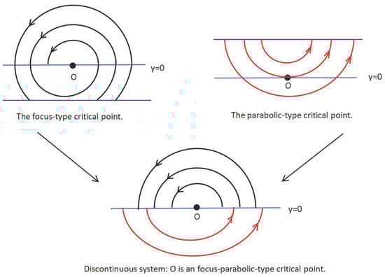
Figure 1. The focus-parabolic-type critical point.

It is known that the classical bifurcation theory is a powerful tool to deal with the limit cycles of smooth systems. However, because of the strong nonlinearities caused by the non-smoothness, the problems of limit cycles for a PWS system are much more complex than those for smooth ones. An important method to investigate the limit cycle problems of the system (1) is the first-return map. To compute the first-return map of the upper–lower subsystem (1), the Lyapunov constants $V_n$ of the system (1) for $n\ge 1$ are defined well. By $V_n$, we can further determine whether the system has a weak center or a weak focus. In general, the index n of the first nonzero $V_n$ for a smooth system is always an odd number $n=2l+1$, in which l is the number of limit cycles bifurcated from the critical point $(0,0)$. However, the index n of $V_n$ of the PWS system may be either odd or even [5]. In [18], Novae and Silva investigated Lyapunov coefficients for monodromic tangential singularities in Filippov vector fields and indicated that the index of the first nonzero $V_n$ for a critical point is always an even number $n=2l+2$, where l represents the number of limit cycles bifurcated from the $(0,0)$. Recently, Chen et al. [19] presented a method based on the Bogdanov–Takens bifurcation theory to compute Lyapunov constants. Furthermore, they also prove that if $(0,0)$ is a cusp, under small quadratic perturbations, the system can bifurcate at least seven limit cycles from the critical point $(0,0)$.

In the past two decades, people have devoted themselves to the study of limit cycles for PWS quadratic and cubic systems (1). Unfortunately, until now, the maximum number of limit cycles for a PWS system with two zones remains unknown. Below, we mention only a few of them when $(0,0)$ is a FF type critical point. As the first results, Coll [20] and Gasull [21] investigated the limit cycles of the planar PWS quadratic system. They obtained at least four and five limit cycles bifurcated from the $(0,0)$, respectively. In [22], Chen and Du investigated a switching system and obtained nine small-amplitude limit cycles bifurcated from the center. Furthermore, the work of [23] showed that at least ten small-amplitude limit cycles can be bifurcated from the center for such a switching system. Planar PWS quadratic systems with five limit cycles bifurcated from the isochronous centers were given by applying the averaging theory in [24]. In [25], Gouveia and Torrerosa investigated isolated crossing periodic orbits in planar piecewise polynomial vector fields defined in two zones separated by a straight line. In particular, they prove that the given system can bifurcate at least thirteen small-amplitude limit cycles from an equilibrium. Da Cruz et al. [26] constructed an example of a PWS quadratic system with one switching line and obtained at least sixteen limit cycles bifurcated from the period annulus of some isochronous quadratic centers. Compared with quadratic PWS systems, more and more people are paying attention to the maximum number of limit cycles for the more complex cubic PWS systems. In [27], Li et al. investigated an FF-type continuous switching PWS system associated with elementary singular points and proved that at least seven limit cycles can be bifurcated from an isochronous center. In [28], Guo et al. developed a method for computing the Lyapunov constants of a planar PWS system and obtained eight limit cycles from two foci. As far as we know, the best lower bound was given in [29] by Huang et al. They proved that at least ten limit cycles for cubic systems and thirteen limit cycles for quartic systems can be bifurcated from the local cyclicity.

For small amplitude limit cycles, in addition to FF-type systems, many scholars have focused their attention on the cases of systems with FP (or PF) and PP-type critical points. It is worth noting that, as pointed out in [5], when the flow of the system (1) has a parabolic contact at a critical point and presents more difficulties, the first-return map may not be analytic. To deal with this problem, the generalized polar coordinates must be used. In [5], Coll et al. constructed an example of planar PWS quadratic systems with an FP-type critical point that bifurcates at least four limit cycles and with a PP-type critical point that bifurcates at least one limit cycle. Han and Zhang [10] investigated the Hopf bifurcation of non-smooth planar systems with FP- and PP-type critical points and obtained two limit cycles. Sun and Du proved in [30] that at least six limit cycles can bifurcate from a weak center and at least nine limit cycles can bifurcate from a weak focus in a planar PWS quadratic system with one switching line. This result improved to ten in [13]. In [18], Novaes and Silva investigated a PWS quadratic system with a PP-type critical point that has five limit cycles bifurcated from $(0,0)$. Then, this result was improved to seven by Fan and Du [31]. In addition, the Hopf bifurcation and stability of PWS systems with a PP-type critical point were investigated in [32,33].

In this paper, we study small-amplitude crossing limit cycles bifurcated from $(0,0)$ in the following planar PWS cubic systems:

$$\begin{array}{c}\hfill \left(\begin{array}{c}\dot{x}\\ \dot{y}\end{array}\right)=\left\{\begin{array}{cc}\left(\begin{array}{c}\lambda x-y-a_3{x}^2+(2a_2+a_4)xy+{\varphi }_1(x,y)\\ x+\lambda y+a_2{x}^2+2a_{3}xy+{\varphi }_2(x,y)\end{array}\right),\hfill & y\ge 0,\hfill \\ \\ \left(\begin{array}{c}1+b_1{x}^2+b_{2}xy+b_3{y}^2\\ 2x+b_4{x}^2+b_{5}xy+b_6{y}^2\end{array}\right),\hfill & y\le 0,\hfill \end{array}\right.\end{array}$$

(2)

where

$$\begin{array}{ccc}\hfill {\varphi }_1(x,y)& =& a_6{y}^3+a_7{x}^{2}y+a_5{y}^2,\hfill \\ \hfill {\varphi }_2(x,y)& =& a_8{x}^3+a_{9}x{y}^2-a_2{y}^2,\hfill \end{array}$$

and $\lambda ,a_2,a_3,a_4,a_5,a_6,a_7,a_8,a_9,b_1,b_2,b_3,b_4,b_5,b_6$ are real parameters. For the system (2), the upper subsystem belongs to a focus-type critical point at $(0,0)$, and the solution of the lower subsystem has a parabolic contact with $y=0$. Thus, $(0,0)$ is a critical point of the FP type based on the definition of an FP-type critical point. Moreover, the orbits near $(0,0)$ of both subsystems of (2) intersect the line $y=0$, indicating there is no grazing or sliding near $(0,0)$. By using the generalized polar coordinates to compute the Lyapunov constants $V_n$, we obtain nine weak focus conditions of order 9 and eleven weak center conditions at $(0,0)$. In addition, we also obtain five conditions under which $(0,0)$ may be a weak center by direct numerical simulation for system (2). Then, we prove that at least nine limit cycles can be bifurcated by applying linear perturbations.

It is easy to see from the known literature that, although there have been a lot of works on limit cycles for FP-type critical points, the considered systems are all quadratic. In this paper, we first investigate the limit cycles of a planar PWS FP-type cubic system with one switching line.

Our paper is organized as follows. In Section 2, we introduce the generalized polar coordinates and give the main results of the paper. The proofs of the main results are given in Section 3 and Section 4. In Section 5, we give some concluding remarks.

2. Preliminaries and the Main Results

To compute the first-return map of system (2), we introduce the $(R,\theta ,1,2)$-generalized polar coordinates, defined by $x=RCs\left(\theta \right),y=R^{2}Sn\left(\theta \right)$, in which $Cs\left(\theta \right)$ and $Sn\left(\theta \right)$ are the solutions of the Cauchy problem:

$$\frac{dCs\left(\theta \right)}{d\theta }=-Sn\left(\theta \right),\frac{dSn\left(\theta \right)}{d\theta }=C{s}^3\left(\theta \right),Cs\left(0\right)=1,Sn\left(0\right)=0.$$

It is easy to verify that $C{s}^4\left(\theta \right)+2S{n}^2\left(\theta \right)=1$ for any $\theta \in \mathbb{R}$. From [20], both $Cs\left(\theta \right)$ and $Sn\left(\theta \right)$ are periodic functions with period $T=2\tau$, where $\tau$ is given by

$$\tau =\frac{\Gamma \left(\frac{1}{2}\right)\Gamma \left(\frac{1}{4}\right)}{\sqrt{2}\Gamma \left(\frac{3}{4}\right)}=\frac{1}{2\sqrt{\pi }}{\left[\Gamma \left(\frac{1}{4}\right)\right]}^2,$$

where $\Gamma \left(s\right)$ is the usual Gamma function for $s\in (0,+\infty )$. Clearly, $Cs\left(0\right)=1$, $Cs\left(\tau \right)=-1$, $Cs\left(2\tau \right)=1,Sn\left(0\right)=Sn\left(\tau \right)=Sn\left(2\tau \right)=0$.

Let $\Delta \left(\theta \right)=C{s}^2\left(\theta \right)+Sn\left(\theta \right)$; then, $\Delta \left(0\right)=\Delta \left(\tau \right)=1$. Let k be any nonzero integer, and define

$$\Lambda (\theta ,k)=\frac{{[\Delta \left(\theta \right)]}^k}{kC{s}^{2k}\left(\theta \right)}.$$

In this paper, we only need the value of $\Lambda (\theta ,k)$ at $\theta =0$ and $\theta =\tau$. Let l be a positive integer and $n>0$ be a constant. For any $0\le i\le l$, we define

$$\begin{array}{c}\hfill a(n,l,i,\theta )=\left\{\begin{array}{cc}\Lambda (\theta ,l-i-n+1),\hfill & l-i-n\ne -1,\hfill \\ \\ ln\left|\frac{\Delta \left(\theta \right)}{C{s}^2\left(\theta \right)}\right|,\hfill & l-i-n=-1.\hfill \end{array}\right.\end{array}$$

Then, we have the following lemma, which was proven in [5].

Lemma 1.

Let l be a positive integer and m be a positive real number such that $m=2n-2l-3$. Then

$$\begin{array}{c}\hfill \int \frac{C{s}^m\left(\theta \right)S{n}^l\left(\theta \right)}{{[\Delta \left(\theta \right)]}^n}d\theta =\sum _{i=0}^l{(-1)}^i\left(\begin{array}{c}l\\ i\end{array}\right)a(n,l,i,\theta )+C,\end{array}$$

where C is an arbitrary integration constant.

To achieve the goal of this paper, we carry out the polar coordinate transformation of the system (2). We transform the upper system of (2) by $x=rcos\theta ,y=rsin\theta$ and obtain

$$\begin{array}{c}\hfill \frac{dr}{d\theta }=\frac{\lambda r+R_1\left(\theta \right)r^2+R_2\left(\theta \right)r^3}{1+{\Theta }_1\left(\theta \right)r+{\Theta }_2\left(\theta \right)r^2},\theta \in [0,\pi ],\end{array}$$

(3)

where

$$\begin{array}{ccc}\hfill R_1\left(\theta \right)& =& (3a_2+a_4){cos}^2\left(\theta \right)sin\left(\theta \right)+(2a_3+a_5)cos\left(\theta \right){sin}^2\left(\theta \right)\hfill \\ & & -a_3{cos}^3\left(\theta \right)-a_2{sin}^3\left(\theta \right),\hfill \\ \hfill R_2\left(\theta \right)& =& (a_7+a_8){cos}^3\left(\theta \right)sin\left(\theta \right)+(a_6+a_9)cos\left(\theta \right){sin}^3\left(\theta \right),\hfill \\ \hfill {\Theta }_1\left(\theta \right)& =& a_2{cos}^3\left(\theta \right)-a_5{sin}^3\left(\theta \right)+3a_3{cos}^2\left(\theta \right)sin\left(\theta \right)\hfill \\ & & -(3a_2+a_4){sin}^2\left(\theta \right)cos\left(\theta \right),\hfill \\ \hfill {\Theta }_2\left(\theta \right)& =& (a_9-a_7){cos}^2\left(\theta \right){sin}^2\left(\theta \right)+a_8{cos}^4\left(\theta \right)-a_6{sin}^4\left(\theta \right).\hfill \end{array}$$

For the lower system of (2), we select a suitable coordinate transformation $(x,y,t)\to (-x,-y,t)$ and transform it to the upper region $\{(x,y)\in {\mathbb{R}}^2:y\ge 0\}$. Then, it has the following form:

$$\begin{array}{c}\hfill \left(\begin{array}{c}\dot{x}\\ \dot{y}\end{array}\right)=\left(\begin{array}{c}-1-b_1{x}^2-b_{2}xy-b_3{y}^2\\ 2x-b_4{x}^2-b_{5}xy-b_6{y}^2\end{array}\right),fory\ge 0.\end{array}$$

(4)

Then, we apply the $(R,\theta ,1,2)$-generalized polar coordinates as described above to the system (4), which yields

$$\begin{array}{c}\hfill \frac{dR}{d\theta }=\frac{G(\theta ,R)R}{1+H(\theta ,R)R},\theta \in [0,\tau ],\end{array}$$

(5)

where $G(\theta ,R)=G_0(\theta ,R)/(2\Delta \left(\theta \right)),H(\theta ,R)=H_0(\theta ,R)/(2\Delta \left(\theta \right))$ with

$$\begin{array}{ccc}\hfill G_0(\theta ,R)& =& -[b_{1}C{s}^5\left(\theta \right)+b_{5}Cs\left(\theta \right)S{n}^2\left(\theta \right)]R^2-b_{3}S{n}^2\left(\theta \right)C{s}^3\left(\theta \right)R^4\hfill \\ & & +[2Cs\left(\theta \right)Sn\left(\theta \right)-C{s}^3\left(\theta \right)]-b_{4}C{s}^2\left(\theta \right)Sn\left(\theta \right)R\hfill \\ & & -[b_{2}C{s}^4\left(\theta \right)Sn\left(\theta \right)+b_{6}S{n}^3\left(\theta \right)]R^3,\hfill \\ \hfill H_0(\theta ,R)& =& (2b_2-b_6)Cs\left(\theta \right)S{n}^2\left(\theta \right)R^2+2b_{3}S{n}^3\left(\theta \right)R^3-b_{4}C{s}^3\left(\theta \right)\hfill \\ & & +(2b_1-b_5)C{s}^2\left(\theta \right)Sn\left(\theta \right)R.\hfill \end{array}$$

To investigate the bifurcation of limit cycles of the system (2), we construct the first-return map $\Pi :{\mathbb{R}}^{+}\to {\mathbb{R}}^{+}$. We first define the positive half-return map ${\Pi }^{+}:{\mathbb{R}}^{+}\to {\mathbb{R}}^{-}$ of system (2) as ${\Pi }^{+}\left(\rho \right)=r^{+}(\rho ,\pi )$, where $r^{+}(\rho ,\theta )$ is the solution of (3) satisfying the initial condition $r^{+}(\rho ,0)=\rho$ with $\rho >0$. Similarly, the negative half-return map ${\Pi }^{-}:{\mathbb{R}}^{-}\to {\mathbb{R}}^{+}$ coincides with the return map induced by the flow of (5) between $\theta =0$ and $\theta =\tau$, which is defined as ${\Pi }^{-}\left(\rho \right)=R^{-}(\rho ,\tau )$, where $R^{-}(\rho ,\theta )$ is the solution of (5) satisfying the initial condition $R^{-}(\rho ,0)=\rho >0$. Thus, the first-return map $\Pi :{\mathbb{R}}^{+}\to {\mathbb{R}}^{+}$ for system (2) is given by $\Pi \left(\rho \right)={\Pi }^{-}\left({\Pi }^{+}\left(\rho \right)\right)$. The displacement function $d:{\mathbb{R}}^{+}\to {\mathbb{R}}^{+}$ is defined by $d\left(\rho \right)=\Pi \left(\rho \right)-\rho$ for $\rho >0$ small enough and can be written as

$$\begin{array}{c}\hfill d\left(\rho \right)=V_1\rho +V_2{\rho }^2+V_3{\rho }^3+\cdots ,\end{array}$$

(6)

where $V_k$ is called the k-th Lyapunov constant of system (2) and $V_1=e^{\lambda \pi }-1$. From [5], it is obvious that we need to compute $V_k$ when $V_1=V_2=\cdots =V_{k-1}=0$. Since $V_1=0$ if and only if $\lambda =0$, we always assume that $\lambda =0$. If $V_1=V_2=\cdots =V_k=0$ and $V_{k+1}\ne 0$, then (0,0) is called a weak focus of order k of system (2). Instead, we call $(0,0)$ a weak center of (2) if $V_j=0$ for all $j\ge 1$. As pointed out in [5,21], there exist at most k limit cycles bifurcated from a weak focus of order k of system (2).

In the following, we will give specific steps to describe how to calculate the Lyapunov constants $V_k$ of system (2) for $k\ge 1$. Equation (3) for $\lambda =0$ can be written as the following form for sufficiently small $r>0$:

$$\begin{array}{c}\hfill \frac{dr}{d\theta }=(R_1\left(\theta \right)+r{R}_2\left(\theta \right))\sum _{k=0}^{\infty }{(-1)}^k{[{\Theta }_1\left(\theta \right)+r{\Theta }_2\left(\theta \right)]}^k{r}^{k+2},\theta \in [0,\pi ].\end{array}$$

(7)

The solution $r^{+}(\rho ,\theta )$ of (3) satisfying the initial condition $r^{+}(\rho ,0)=\rho >0$ can be expanded as

$$\begin{array}{c}\hfill r^{+}(\rho ,\theta )=\sum _{k=1}^{\infty }{r}_k^{+}\left(\theta \right){\rho }^k,\theta \in [0,\pi ].\end{array}$$

(8)

It is clear that $r_1^{+}\left(0\right)=1$ and $r_k^{+}\left(0\right)=0$ for any $k\ge 2$. Furthermore, we can compute the $r_k^{+}\left(\theta \right)$ for $k\ge 1$ by substituting (8) into (7) and comparing the coefficients of ${\rho }^k$. Then,

$$\Pi \left(\rho \right)=r_1^{+}\left(\pi \right)\rho +r_2^{+}\left(\pi \right){\rho }^2+r_3^{+}\left(\pi \right){\rho }^3+\cdots .$$

For sufficiently small $R>0$, (5) can be written as

$$\begin{array}{c}\hfill \frac{dR}{d\theta }=\sum _{k=1}^{\infty }{T}_k\left(\theta \right)R^k,\theta \in [0,\tau ],\end{array}$$

(9)

where

$$T_1\left(\theta \right)=\frac{2Cs\left(\theta \right)Sn\left(\theta \right)-C{s}^3\left(\theta \right)}{2\Delta \left(\theta \right)}=-\frac{{\Delta }^{\prime }\left(\theta \right)}{2\Delta \left(\theta \right)}.$$

According to the Lemma 1 of [5], system (9) can be transformed by the change of variables $r=Rexp\left(-{\int }_0^{\theta }{T}_1\left(\varphi \right)d\varphi \right)$ to the following form:

$$\begin{array}{c}\hfill \frac{dr}{d\theta }=\sum _{k=2}^{\infty }{R}_k\left(\theta \right)r^k,\end{array}$$

(10)

where $R_k\left(\theta \right)=T_k\left(\theta \right)/{[\Delta \left(\theta \right)]}^{\frac{k-1}{2}}$. Let $r(\rho ,\theta )$ be the solution of (10) satisfying the initial condition $r(\rho ,0)=\rho >0$, which can be written as

$$\begin{array}{c}\hfill r(\rho ,\theta )=\rho +\sum _{k=2}^{\infty }{u}_k\left(\theta \right){\rho }^k,\end{array}$$

(11)

where $u_k\left(0\right)=0$ for $k\ge 2$. Let $R(\rho ,\theta )$ be the solution of (9) satisfying $R(\rho ,0)=\rho$. Then, it is clear that

$$\begin{array}{c}\hfill R(\rho ,\theta )=\rho +\sum _{k=1}^{\infty }{w}_k\left(\theta \right){\rho }^k={\left[\Delta \left(\theta \right)\right]}^{-\frac{1}{2}}\left[\rho +\sum _{k=2}^{\infty }{u}_k\left(\theta \right){\rho }^k\right].\end{array}$$

It is worth noting that $u_k\left(\theta \right)$ can be computed by substituting (11) into (10) and comparing the coefficients of ${\rho }^k$ for $k\ge 2$. Then, we have

$$w_1\left(\theta \right)={\left[\Delta \left(\theta \right)\right]}^{-\frac{1}{2}}-1,w_k\left(\theta \right)={\left[\Delta \left(\theta \right)\right]}^{-\frac{1}{2}}{u}_k\left(\theta \right).$$

It is easy to see that $w_1\left(\tau \right)=0$, and thus

$${\Pi }^{-}\left(\rho \right)=R(\rho ,\tau )=\rho +w_2\left(\tau \right){\rho }^2+w_3\left(\tau \right){\rho }^3+\cdots .$$

Since $\Delta \left(\tau \right)=1$, we have $w_k\left(\tau \right)=u_k\left(\tau \right)$ for any $k\ge 2$.

Below, let $\zeta =(\lambda ,a_2,\cdots ,a_9,b_1,\cdots ,b_6)\in {\mathbb{R}}^{15}$ be the parameters of system (2). Let $\parallel v\parallel =\sqrt{v{v}^T}$ be the usual Euclidean norm for any row vector $v\in {\mathbb{R}}^n$. Define

$$\begin{array}{ccc}\hfill {\mathcal{H}}_1& =& 5,848,384a_2^6-92,191b_5^6+17,280a_2^4{b}_5+28,512a_2^2{b}_5^2+3456b_5^3,\hfill \\ \hfill {\mathcal{H}}_2& =& 19,644,724a_2^6-18,069,436b_1^6+1,227,015a_2{b}_1+33,480a_2^2{b}_1^2+32,481b_1^3,\hfill \\ \hfill {\mathcal{H}}_3& =& a_2^7{a}_9+\frac{292}{3465}{a}_2^5{a}_9^2+\frac{304}{5775}{a}_9^3{a}_2^3+\frac{128}{12,375}{a}_9^4{a}_2-\frac{6,109,749}{140}{a}_2^{13}{a}_9,\hfill \\ \hfill {\mathcal{H}}_4& =& 1,028,875,621,851a_{12}{a}_5^2-97,988,154,462a_2^{11}{b}_6-87,282,174a_2^6{a}_5^2-39,150,216a_2^4{a}_5^4\hfill \\ & & +203,494,032a_2{a}_5^6+609,420,672a_5^8+11,800,448a_2^5{b}_6+7,892,640a_2^3{a}_5^2{b}_6\hfill \\ & & -22,861,440a_2{a}_5^4{b}_6+2,177,280a_5^2{b}_6^2,\hfill \\ \hfill {\mathcal{H}}_5& =& 48,334,635,008a_4^{14}+84,585,611,264a_4^{12}{a}_7+47,579,406,336a_4^{10}{a}_7^2-25,110a_7^4\hfill \\ & & -501,814,0512a_4^4{a}_7^5-8,912,960a_4^8-940,901,346a_4^2{a}_7^6+7,171,600a_4^6{a}_7\hfill \\ & & -11,151,423,360a_4^6{a}_7-67,207,239a_7^7-621,432a_4^4{a}_7^2-317,844a_4^2{a}_7^3,\hfill \\ \hfill {\mathcal{H}}_6& =& -\frac{2,852,912}{280,665}{b}_6{a}_4^6+\frac{63}{693}{a}_4^3{b}_6^2+\frac{1,098,514,432}{25,515}{a}_4^{12}{b}_6-\frac{31,832}{8019}{a}_4^9\hfill \\ & & +\frac{549,257,216}{25,515}{a}_4^{15}.\hfill \end{array}$$

(12)

We are now ready to present the weak center conditions and weak focus conditions for system (2). Furthermore, we give the number of limit cycles in a small neighborhood of $(0,0)$ under weak center conditions and weak focus conditions.

Theorem 1.

(1) System(2) has a weak center at $(0,0)$ if one of the following conditions is satisfied:

$$\begin{array}{ccc}\hfill \left({\mathcal{C}}_1\right)& & a_4=a_8=b_2=b_6=0,a_7=-a_9,b_4=2a_2,b_5=-2b_1;\hfill \\ \hfill \left({\mathcal{C}}_2\right)& & a_4=a_8=0,a_7=-a_9,b_4=-b_5=2a_2=2b_1,b_2=-2b_6;\hfill \\ \hfill \left({\mathcal{C}}_3\right)& & a_4=a_8=0,a_7=-a_9,b_4=b_5=2a_2=-2b_1,b_2=-2b_6;\hfill \\ \hfill \left({\mathcal{C}}_4\right)& & a_2=a_4=b_1=b_4=b_5=0,a_7=-a_9,b_2=-2b_6,\hfill \\ \hfill \left({\mathcal{C}}_5\right)& & a_2=a_4=a_8=b_1=b_4=b_5=0,a_3=a_5,b_2=-2b_6;\hfill \\ \hfill \left({\mathcal{C}}_6\right)& & a_2=a_4=a_8=b_4=0,a_3=a_5,b_2=-2b_6,b_5=-2b_1=-9a_5^2-5a_6,\hfill \\ & & a_9=-a_7=(9a_5^2+10a_6)/7;\hfill \\ \hfill \left({\mathcal{C}}_7\right)& & a_3=a_5=a_2=a_8=a_6=b_2=b_6=0,b_4=2a_4,b_5=-2b_1,a_7=2a_4^2;\hfill \\ \hfill \left({\mathcal{C}}_8\right)& & a_3=a_5=a_2=a_8=a_6=0,b_2=-2b_6,b_5=-b_4=-2b_1=-2a_4,\hfill \\ & & a_7=2a_4^2;\hfill \\ \hfill \left({\mathcal{C}}_9\right)& & a_3=a_5=a_2=a_8=a_6=0,b_2=-2b_6,b_5=b_4=-2b_1=2a_4,\hfill \\ & & a_7=2a_4^2;\hfill \\ \hfill \left({\mathcal{C}}_{10}\right)& & a_3=a_5=a_6=b_1=b_4=b_5=0,a_4=-a_2,a_9=-2a_7=2a_8,b_2=-2b_6;\hfill \\ \hfill \left({\mathcal{C}}_{11}\right)& & a_3=a_5=a_6=b_2=b_6=b_4=0,a_4=-a_2,a_9=-2a_7=2a_8,b_5=-2b_1.\hfill \end{array}$$

(2) System(2) has a weak focus of order nine at $(0,0)$ if one of the following conditions is satisfied:

$$\begin{array}{ccc}\hfill \left({\mathcal{F}}_1\right)& & a_4=a_8=b_6=0,a_7=-a_9,b_4=2a_2,b_1=-(5a_2^2+2b_5),\hfill \\ & & b_2=a_2(5a_2^2+\frac{3}{2}{b}_5),b_3=\frac{4a_2^2{b}_5-b_5^2}{12},{\mathcal{H}}_1{a}_2(10a_2^2+3b_5)\ne 0;\hfill \\ \hfill \left({\mathcal{F}}_2\right)& & a_4=b_6=0,a_7=-a_9,b_4=2a_2,b_5=-2b_1,a_8=\frac{12a_2^2+2b_1}{7},\hfill \\ & & b_2=-\frac{a_2(30a_2^2+5b_1)}{28},b_3=\frac{589}{224}{a}_2^4+\frac{5}{16}{a}_2^2{b}_1+\frac{27}{224}{b}_1^2,\hfill \\ & & (6a_2^2+b_1){\mathcal{H}}_2\ne 0;\hfill \\ \hfill \left({\mathcal{F}}_3\right)& & a_4=b_6=0,b_4=2a_2,a_7=-a_9,3b_5=6b_1=-6a_8=-16a_2^2,\hfill \\ & & b_2=2a_2^3,b_3=\frac{146}{49}{a}_2^4,\frac{501,943}{56,133}{a}_2^9-\frac{70,304,923,648}{18,600,435}{a}_2^{15}\ne 0;\hfill \\ \hfill \left({\mathcal{F}}_4\right)& & a_3=a_4=a_5=a_8=0,b_4=2a_2,b_5=-2b_1=9a_2^2,b_2=-2b_6,\hfill \\ & & a_6=-7a_7/10,b_2{b}_6(531,441a_2^6-64)\ne 0;\hfill \\ \hfill \left({\mathcal{F}}_5\right)& & a_3=a_4=a_5=a_6=a_7=a_8=b_6=0,b_4=2a_2,b_5=-2b_1,\hfill \\ & & a_9=\frac{9}{2}{a}_a^2+b_1,b_2=\frac{9}{2}{a}_2^3+a_2{b}_1,b_3=\frac{1}{32}(13a_2^4+6a_2^2{b}_1+5b_1^2),\hfill \\ & & {\mathcal{H}}_3\ne 0;\hfill \\ \hfill \left({\mathcal{F}}_6\right)& & a_4=a_8=0,a_3=a_5,b_4=2a_2,b_5=-2b_1=9a_2^2,a_9=12a_5,\hfill \\ & & b_2=21a_2{a}_5^2,b_3=\frac{349}{128}(a_2^4-452a_2^2{a}_5^2+3240a_5^4+48a_2{b}_6),{\mathcal{H}}_4\ne 0;\hfill \\ \hfill \left({\mathcal{F}}_7\right)& & a_4=a_8=0,a_3=a_5,b_2=-2b_6,b_5=-2b_1=9a_2^2+5a_6+7a_7,\hfill \\ & & b_4=2a_2,a_9=-a_7=(9a_5^2+10a_6)/7,a_2{b}_6(531,441a_2^6-64)\ne 0;\hfill \\ \hfill \left({\mathcal{F}}_8\right)& & a_2=a_3=a_5=a_6=a_8=0,b_5=-2b_1=8a_4^2-3a_7,b_4=2a_4,\hfill \\ & & b_2=-a_4^3+\frac{1}{2}{a}_4{a}_7,b_3=\frac{1}{128}(324a_4^4+268a_4{a}_7+21a_7^2),a_4{\mathcal{H}}_5\ne 0;\hfill \\ \hfill \left({\mathcal{F}}_9\right)& & a_2=a_6=a_8=0,a_3=a_5,b_4=2a_4,a_9=a_7=-3a_5^2,\hfill \\ & & b_5=-2b_1=8a_4^2,b_2=-a_4^3-2b_6,b_3=\frac{81}{32}{a}_4^4+\frac{3}{8}{a}_4{b}_6,{\mathcal{H}}_6\ne 0.\hfill \end{array}$$

Theorem 2.

(1) For the weak center of system (2) under conditions $({\mathcal{C}}_i,i=1,\cdots ,11)$, there exists ${\zeta }_0$ satisfying the weak center condition such that for any $\zeta \in {\mathbb{R}}^{15}$ with a $\parallel \zeta -{\zeta }_0\parallel >0$ that is sufficiently small, system (2) generates 9, 9, 9, 6, 6, 8, 9, 9, 9, 8, 8 limit cycles, respectively. (2) For the weak focus of system (2) under conditions $({\mathcal{F}}_j,j=1,\cdots ,9)$, there exists ${\zeta }_0$ satisfying the weak focus condition such that for any $\zeta \in {\mathbb{R}}^{15}$ with $\parallel \zeta -{\zeta }_0\parallel >0$ that is sufficiently small, the bifurcation of system (2) produces 9, 9, 9, 8, 8, 9, 8, 9, 9 limit cycles, respectively.

Remark 1.

When the following conditions are satisfied

$$\begin{array}{c}\hfill \begin{array}{cc}\hfill \left({\mathcal{A}}_1\right)& a_4=a_2=b_4=b_2=b_6=0;\hfill \\ \hfill \left({\mathcal{A}}_2\right)& a_2=a_4=b_4=0,b_2=-2b_6,b_5=-2b_1;\hfill \\ \hfill \left({\mathcal{A}}_3\right)& a_2=a_6=a_8=b_2=b_6=0,a_3=a_5,b_4=2a_4,b_5=-2b_1,\hfill \\ & a_7=a_9=2a_4^2-3a_5^2;\hfill \\ \hfill \left({\mathcal{A}}_4\right)& a_2=a_6=a_8=0,b_2=-2b_6,a_3=a_5,b_4=2a_4,b_5=-2b_1=-2a_4,\hfill \\ & a_7=a_9=2a_4^2-3a_5^2;\hfill \\ \hfill \left({\mathcal{A}}_5\right)& a_2=a_6=a_8=0,b_2=-2b_6,a_3=a_5,b_4=2a_4,b_5=-2b_1=2a_4,\hfill \\ & a_7=a_9=2a_4^2-3a_5^2,\hfill \end{array}\end{array}$$

we have $V_1=V_2=\cdots =V_{10}=0$. Here, we only conjecture that under conditions $({\mathcal{A}}_k,k=1\cdots ,5)$, $(0,0)$ is a weak center of system (2) with some numerical examples. However, we are not able to prove this rigorously by constructing the first integral for the upper and lower subsystems of (2).

Through a large number of numerical experiments, we see that $({\mathcal{A}}_k,k=1,\cdots ,5)$ are weak center conditions. In the following, we provide some numerical simulations. Under condition $\left({\mathcal{A}}_1\right)$, we choose a set of parameters $A_1:a_2=a_4=b_2=b_4=b_6=0$, $a_3=2$, $a_5=5,a_7=3,a_8=10,a_9=-5,b_1=3,b_3=3,b_5=6$ and plot the diagram shown in Figure 2a. Under condition $\left({\mathcal{A}}_2\right)$, we choose a set of parameters $A_2:a_2=a_4=b_4=0$, $a_3=2$, $a_5=5,a_6=1,a_7=3,a_8=10,a_9=-5,b_1=3,b_2=-2,b_3=3,b_5=6,b_6=1$ and plot the diagram shown in Figure 2b Under condition $\left({\mathcal{A}}_3\right)$, we choose a set of parameters $A_3:a_2=a_6=a_8=b_2=b_6=0,a_3=2,a_4=3,a_5=2,a_7=a_9=6,b_1=10$, $b_3=111$, $b_4=6,b_5=-20$ and plot the diagram shown in Figure 2c. Under condition $\left({\mathcal{A}}_4\right)$, we choose a set of parameters $A_4:a_2=a_6=a_8=0,a_3=a_5=5,b_2=-6,b_3=3,a_4=4$, $b_4=8$, $b_1=4,b_5=-8,a_7=a_9=-43,b_6=3$ and plot the diagram shown in Figure 2d. Under condition $\left({\mathcal{A}}_5\right)$, we choose a set of parameters $A_5:a_2=a_6=a_8=0$, $a_3=a_5=5$, $b_2=-6,b_3=3,a_4=3,b_4=6,b_1=-3,b_5=6,a_7=a_9=-57,b_6=3$ and plot the diagram shown in Figure 2e. From Figure 2, it is easy to see that under conditions $({\mathcal{A}}_i,i=1,\cdots ,5)$, $(0,0)$ is a weak center.

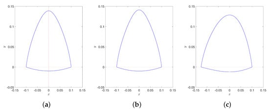
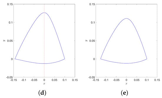
Figure 2. Phase portraits of the system (2) for different parameter conditions $A_1,A_2,A_3,A_4$, and $A_5$. (a) Parameters are as in $A_1$. (b) Parameters are as in $A_2$. (c) Parameters are as in $A_3$. (d) Parameters are as in $A_4$. (e) Parameters are as in $A_5$.

Theorem 3.

For each $k=1,2,3,4,5$, there exists a ${\zeta }_0\in {\mathbb{R}}^{15}$ satisfying the conditions $\left({\mathcal{A}}_k\right)$ such that for any $\zeta \in {\mathbb{R}}^{15}$ with $\parallel \zeta -{\zeta }_0\parallel >0$ that is sufficiently small, system (2) has 5, 7, 9, 9, 9 limit cycles in a small neighborhood of $(0,0)$, respectively.

3. Proof of Theorem 1

In this section, we prove Theorem 1 by investigating the Lyapunov constants of system (2) and further obtain the conditions of weak center and weak focus. We also prove that $(0,0)$ is a weak center by constructing an explicit first integral when weak center conditions are satisfied.

Proof of Theorem 1.

The Lyapunov constants $V_k$ for $k\ge 2$ can be computed with the special constants using the Gröbner basis of Maple with the term order $(a_2,a_3,a_4,a_5,a_6,a_7,a_8,a_9,b_1$, $b_2,b_3,b_4,$$b_5,b_6)$. Since system (2) is cubic, the Lyapunov constants $V_k$ for $k\ge 4$ are very complex, so we first compute $V_2$ and $V_3$ for system (2) with $\lambda =0$, which are given by

$$\begin{array}{ccc}\hfill V_2& =& \frac{2}{3}{a}_2+\frac{2}{3}{a}_4-\frac{1}{3}{b}_4,\hfill \\ \hfill V_3& =& -\frac{\pi }{8}{a}_4(a_3-a_5).\hfill \end{array}$$

We first compute the common zeros of $V_2$ and $V_3$. From $V_2=V_3=0$, we obtain the following two conditions:

(H1)

$a_4=0$ and $b_4=2a_2$.

(H2)

$a_3=a_5$ and $b_4=2(a_2+a_4)$.

Case 1: Condition (H1) is satisfied.

Under condition (H1), we have

$$\begin{array}{ccc}\hfill V_4& =& \frac{1}{15}(4a_7-10a_8+4a_9-4b_1-2b_5)a_2-\frac{4}{15}{b}_2-\frac{8}{15}{b}_6,\hfill \\ \hfill V_5& =& -\frac{5}{12}(a_3-a_5)\pi \left[\left(a_8+\frac{2}{5}{b}_1+\frac{1}{5}{b}_5\right)+\frac{2}{5}{b}_2+\frac{4}{5}{b}_6\right].\hfill \end{array}$$

When $V_4=0$, we obtain

$$b_2=(a_7-\frac{5}{2}{a}_8+a_9-b_1-\frac{1}{2}{b}_5)a_2-2b_6.$$

Substituting $b_2$ into the expression of $V_5$, we obtain

$$\begin{array}{c}\hfill V_5=-\frac{\pi }{6}{a}_2(a_7+a_9)(a_3-a_5).\end{array}$$

(13)

We consider the following three cases:

(1) If $a_2=0$, then from (13) and by direct computations, we have $V_2=V_3=V_4=V_5=0$ and

$$V_6=-\frac{8}{105}{b}_6(2b_1+b_5).$$

It is easy to see that $V_6=0$ implies that $b_6=0$ or $b_5=-2b_1$. In either case, we have $V_2=V_3=\cdots =V_{10}=0$ and obtain conditions $\left({\mathcal{A}}_1\right)$ and $\left({\mathcal{A}}_2\right)$.

(2) If $a_7=-a_9$, we have $V_5=0$ and $V_7=0$ and further obtain

$$\begin{array}{ccc}\hfill V_6& =& \frac{1}{105}(-120a_8-20b_1-10b_5)a_2^3+\frac{1}{105}\left[-4b_1^2+(-40a_8-10b_5)\right]b_1\hfill \\ & & +70a_8^2-108a_8{b}_5{a}_2-\frac{16}{105}\left(b_1+\frac{b_5}{2}\right)b_6.\hfill \end{array}$$

(14)

Since (14) is quite complex, we will only discuss the following cases:

(2.1) We first assume that $a_8=b_6=0$ and further obtain

$$\begin{array}{c}\hfill V_6=-\frac{2}{105}(5a_2^2+b_1+2b_5)(2b_1+b_5)a_2.\end{array}$$

(15)

If $a_2=0$, then we obtain $\left({\mathcal{A}}_1\right)$. Let $a_2\ne 0$; $V_6=0$ implies that $b_5=-2b_1$ or $b_1=-(5a_2^2+2b_5)$. If $b_5=-2b_1$, then we obtain condition $\left({\mathcal{C}}_1\right)$. If $b_1=-(5a_2^2+2b_5)$, then $V_2=V_3=V_4=V_5=V_6=V_7=0$ and

$$\begin{array}{ccc}\hfill V_8& =& -\frac{4}{945}(4a_2^2{b}_5-b_5^2-12b_3)a_2(10a_2^2+3b_5),\hfill \\ \hfill V_9& =& -\frac{8}{945}(4a_2^2{b}_5-b_5^2-12b_3)a_2^2(10a_2^2+3b_5).\hfill \end{array}$$

Then, under the condition $a_2\ne 0$, $V_8=V_9=0$ implies that $b_5=-10/3a_2^2$ or $b_3=(4a_2^2-b_5)b_5/12$.

When $b_3=(4a_2^2-b_5)b_5/12$ and $b_5\ne -10/3a_2^2$, we have $V_2=V_3=V_4=V_5=V_6=V_7=V_8=V_9=0$ and

$$V_{10}=\frac{1}{2,245,320}(10a_2^2+3b_5)a_2{\mathcal{H}}_1,$$

where ${\mathcal{H}}_1$ is given by (12). Hence, when condition $\left({\mathcal{F}}_1\right)$ is satisfied, $V_2=\cdots =V_9=0$ and $V_{10}\ne 0$, it shows that $(0,0)$ is a weak focus of order 9 for system (2). If $b_5=-10/3a_2^2$, we obtain $b_5=-2b_1$. Furthermore, we obtain $\left({\mathcal{C}}_1\right)$ again.

(2.2) If $b_5=-2b_1$, then $V_6$ of (14) can be written in the following form:

$$\begin{array}{c}\hfill V_6=-\frac{2}{21}{a}_2{a}_8(12a_2^2-7a_8+2b_1).\end{array}$$

(16)

From $V_6=0$ and $a_2\ne 0$, we obtain $a_8=0$ or $a_8=(12a_2^2+b_1)/7$. If $a_8=0$, then we have $V_6=V_7=V_8=V_9=0$ and

$$V_{10}=\frac{268,192}{25,515}{b}_6(b_1^6-a_2^6).$$

If $b_6=0$, we obtain condition $\left({\mathcal{C}}_1\right)$ again. If $b_1^6=a_2^6$, then we obtain conditions $\left({\mathcal{C}}_2\right)$ and $\left({\mathcal{C}}_3\right)$. If $a_8=(12a_2^2+2b_1)/7$, by direct computation, we have $V_6=V_7=0$ and

$$\begin{array}{ccc}\hfill V_8& =& \frac{4}{9261}{a}_2(6a_2^2+b_1)(589a_2^4+70a_2^2{b}_1+84a_2{b}_6+27b_1^2-224b_3),\hfill \\ \hfill V_9& =& \frac{8}{9261}{a}_2^2(6a_2^2+b_1)(589a_2^4+70a_2^2{b}_1+84a_2{b}_6+27b_1^2-224b_3).\hfill \end{array}$$

(17)

Here, $V_8=V_9=0$ implies that $b_1=-6a_2^2$ or

$$b_3=\frac{589a_2^4+70a_2^2{b}_1+84a_2{b}_6+27b_1^2}{226}.$$

It is easy to see that $b_1=-6a_2^2$ implies that $a_8=0$. This case has been discussed above. Now, we assume that $b_1\ne -6a_2^2$ and $b_3=(589a_2^4+70a_2^2{b}_1+84a_2{b}_6+27b_1^2)/226.$ Thus, we have $V_8=V_9=0$. Since the expression of $V_{10}$ is too complex, to simplify it, we set $b_6=0$. Then, we obtain

$$V_{10}=-\frac{4}{19,253,619}{a}_2(6a_2^2+b_1){\mathcal{H}}_2,$$

where ${\mathcal{H}}_2$ is given by (12). Consequently, when $\left({\mathcal{F}}_2\right)$ is satisfied, $V_2=\cdots =V_9=0$ and $V_{10}\ne 0$, implying that $(0,0)$ is a weak focus of order 9 of system (2).

(2.3) If $3b_5=6b_1=-6a_8=-16a_2^2$, $V_6,V_8$ and $V_9$ can be written as follows:

$$\begin{array}{ccc}\hfill V_6& =& \frac{256}{315}{a}_2{b}_6,\hfill \\ \hfill V_8& =& \frac{256}{2835}{a}_2^3{b}_3+\frac{1,309,856}{416,745}{a}_2^4{b}_6-\frac{584}{2835}{a}_2^7,\hfill \\ \hfill V_9& =& -\frac{1168}{2835}{a}_2^8+\frac{2,619,712}{416,745}{b}_6{a}_2^5-\frac{4096}{2205}{a}_2^2{b}_6^2+\frac{512}{2835}{a}_2^4{b}_3.\hfill \end{array}$$

If $a_2=0$, we obtain a special case of $\left({\mathcal{C}}_2\right)$ and $\left({\mathcal{C}}_3\right)$. Under the condition $a_2\ne 0$, $V_6=0$ implies that $b_6=0$, and thus, we have $V_2=V_3=V_4=V_5=V_6=V_7=0$ and

$$\begin{array}{ccc}\hfill V_8& =& \frac{a_2^3}{2835}(256b_3-582a_2^4),\hfill \\ \hfill V_9& =& \frac{a_2^4}{2835}(256b_3-584a_2^4),\hfill \\ \hfill V_{10}& =& \frac{17,608,733,254,144}{1,755,370,126,125}{a}_2^5{b}_3-\frac{70,304,923,648}{18,600,435}{a}_2^{15}-\frac{24,473,368,231,616}{1,755,370,126,125}{a}_2^9.\hfill \end{array}$$

Let $b_3=146a_2^4/49$, then $V_8=V_9=0$ and

$$V_{10}=\frac{501,943}{56,133}{a}_2^9-\frac{70,304,923,648}{18,600,435}{a}_2^{15}.$$

If $V_{10}\ne 0$, then under the condition $\left({\mathcal{F}}_3\right)$, $(0,0)$ is a weak focus of order 9 of system (2).

(2.4) If $a_2=b_1=0$, we can simplify the expression of (14) and obtain $V_8$ and $V_9$ as follows:

$$\begin{array}{ccc}\hfill V_6& =& -\frac{8}{105}{b}_5{b}_6,\hfill \\ \hfill V_8& =& \frac{16}{9261}{b}_5{b}_6(25b_3+13a_8),\hfill \\ \hfill V_9& =& \frac{128}{735}{b}_5{b}_6^2,\hfill \\ \hfill V_{10}& =& \frac{b_5{b}_6}{13,652,878,758,750}(2,242,304,073,625b_5^5+148,192,753,010,400a_8^2\hfill \\ & & +20,830,976,207,320a_8{b}_5-3,187,644,324,168b_5^2+345,029,765,600b_3).\hfill \end{array}$$

If $b_5=0$ or $b_6=0$, then $V_2=\cdots =V_{10}=0$. Thus, we obtain conditions $\left({\mathcal{C}}_4\right)$ and $\left({\mathcal{A}}_1\right)$, respectively.

(3) If $a_3=a_5$, then from (13) and by direct computations, we have $V_2=V_3=V_4=V_5=0$ and

$$\begin{array}{ccc}\hfill V_6& =& \frac{1}{105}\left[20a_7^2+136a_5^2+40a_6+12a_8+12a_9+16b_1+4b_5{a}_7-8a_9^2\right.\hfill \\ & & +(36a_5^2+40a_6+12a_8+16b_1+4b_5)a_9-4b_1^2-10(4a^8+b_5)b_1\hfill \\ & & \left.+70a_8^2-10a_8{b}_5-4b_5^2\right]a_2+\frac{1}{105}(36a_7-120a_8+36a_9-20b_1\hfill \\ & & -10b_5)a_2^3.\hfill \end{array}$$

(18)

We only consider the case of $a_8=0$ and $b_5=-2b_1$ due to computational complexity.

If $a_8=0$ and $b_5=-2b_1$, then the expression $V_6$ of (18) has the following form:

$$V_6=\frac{4}{105}{a}_2(a_7+a_9)(9a_2^2+9a_5^2+10a_6+5a_7-2a_9+2b_1).$$

Here, $V_6=0$ implies that $a_2=0$ or $a_7=-a_9$ or

$$\begin{array}{c}\hfill a_9=\frac{1}{2}(9a_2^2+9a_5^2+7a_7)+5a_6+b_1.\end{array}$$

(19)

If $a_2=0$, then, by direct computation, it is easy to see that $V_2=\cdots =V_9=0$ and

$$V_{10}=\frac{268,192}{25,515}{b}_1^6{b}_6.$$

Thus, $V_{10}=0$ implies that $b_1=0$ or $b_6=0$. In either case, we have $V_2=\cdots =V_{10}=0$ by further computations. Thus, we obtain conditions $\left({\mathcal{C}}_5\right)$ and $\left({\mathcal{A}}_1\right)$. If $a_7=-a_9$, then by direct computations, we obtain $\left({\mathcal{C}}_2\right)$ and $\left({\mathcal{C}}_3\right)$ again. If (19) is satisfied, then $V_6=0$. In addition, we obtain

$$\begin{array}{ccc}\hfill V_7& =& \frac{5}{384}{a}_2{a}_5\pi (9a_2^2+9a_5^2+12a_6+3a_7+2b_1)(9a_2^2+9a_5^2\hfill \\ & & +10a_6+7a_7+2b_1).\hfill \end{array}$$

(20)

Since $a_2\ne 0$, $V_7=0$ implies that $a_5=0$ or $b_1=-(9a_2^2+9a_5^2+12a_6+3a_7)/2$ or $b_1=-(9a_2^2+9a_5^2+10a_6+7a_7)/2$.

Below, we consider different cases for $V_7=0$.

(3.1) If $a_5=0$, then $V_7=0$. We also obtain

$$\begin{array}{ccc}\hfill V_8& =& -\frac{2}{945}{a}_2(9a_2^2+10a_6+7a_7+2b_1)(13a_2^4-174a_2^2{a}_6-18a_2^2{a}_7+6a_2^2{b}_1\hfill \\ & & +12a_2{b}_6-168a_6^2-86a_6{a}_7-32a_6{b}_1-6a_7^2+5b_1^2-32b_3).\hfill \end{array}$$

(21)

Under condition $a_2\ne 0$, then $V_8=0$ implies that $b_1=-(9a_2^2+10a_6+7a_7)/2$ or

$$\begin{array}{ccc}\hfill b_3& =& \frac{1}{32}\left[13a_2^4-174a_2^2{a}_6-18a_2^2{a}_7+6a_2^2{b}_1+12a_2{b}_6-168a_6^2\right.\hfill \\ & & \left.-86a_6{a}_7-32a_6{b}_1-6a_7^2+5b_1^2\right].\hfill \end{array}$$

(22)

If $b_1=-(9a_2^2+10a_6+7a_7)/2$, then we obtain $V_8=V_9=0$. Since the expression of $V_{10}$ is quite complex, we give some special cases here. If $b_6=0$, then $V_{10}=0$, and we achieve condition $\left({\mathcal{C}}_1\right)$ again. If $a_6=-7a_7/10$, then we have

$$V_{10}=\frac{8381}{51,030}{b}_6{b}_2^6(531,441a_2^6-64).$$

Under condition $b_2{b}_6\ne 0$, if $a_2^6\ne 64/531441$, then $V_{10}\ne 0$. Under the condition $\left({\mathcal{F}}_4\right)$, $(0,0)$ is a weak focus of order 9 of system (2).

If (22) is satisfied and if $a_6=a_7=b_6=0$, then we obtain

$$V_{10}={\mathcal{H}}_3,$$

where ${\mathcal{H}}_3$ is given by (12). If ${\mathcal{H}}_3\ne 0$, then $(0,0)$ is a weak focus of order 9 of system (2) when the condition $\left({\mathcal{F}}_5\right)$ is satisfied.

(3.2) If $b_1=-(9a_2^2+9a_5^2+12a_6+3a_7)/2$, then $V_7=0$. Then, we obtain

$$\begin{array}{ccc}\hfill V_8& =& \frac{1}{945}{a}_2(a_6-2a_7)({\Delta }_1-128b_3),\hfill \end{array}$$

where

$$\begin{array}{ccc}\hfill {\Delta }_1& =& 349a_2^4+538a_2^2{a}_5^2+189a_5^4+816a_2^2{a}_6+162a_2{a}_7+504a_5^2{a}_6\hfill \\ & & +126a_5^2{a}_7+48a_2{b}_6+816a_6^2+208a_6{a}_7+21a_7^2.\hfill \end{array}$$

Under condition $a_2\ne 0$, $V_8=0$ implies that $a_6=2a_7$ or $b_3={\Delta }_1/128$.

If $a_6=2a_7$, then we obtain $V_8=V_9=0$ and the expression of $V_{10}$, where $V_{10}$ is quite complex and has many terms. Thus, we only give two cases. If $b_6=0$, then we obtain the condition $\left({\mathcal{C}}_1\right)$. If $a_7=-a_5^2/3$, then we obtain the weak focus condition $\left({\mathcal{F}}_4\right)$.

If $b_3={\Delta }_1/128$, then by direct computation, we obtain $V_8=0$ and

$$V_9=-\frac{1}{24}{a}_2{a}_5{a}_6(a_6-2a_7)(a_7+3a_6)\pi .$$

We have investigated the case of $a_2=a_5=a_6=0$ and $a_6=2a_7$ above. Thus, $V_9=0$ implies that $a_7=-3a_6$. When $a_7=-3a_6$, we find that the expression of $V_{10}$ is quite complex. To simplify $V_{10}$, let $a_6=-3a_5^2$, we have

$$V_{10}=-\frac{a_2}{1,122,660}{\mathcal{H}}_4,$$

where ${\mathcal{H}}_4$ is given by (12). Under condition $\left({\mathcal{F}}_6\right)$, $(0,0)$ is a weak focus of order 9 of system (2).

(3.3) If $b_1=-(9a_2^2+9a_5^2+10a_6+7a_7)/2$, then we obtain $V_8=V_9=0$ and $V_{10}$. Here, the expression of $V_{10}$ is rather complex. To simplify it, let $a_7=-(9a_5^2+10a_6)/7$, then we get

$$V_{10}=\frac{8183}{51,030}{b}_6{a}_2^6(531,441a_2^6-64).$$

Here, $V_{10}=0$ implies that $a_2=0$ or $b_6=0$ or $a_2^6=64/531,441$. Thus, if $a_2{b}_6=0$, then $V_{10}=0$. Furthermore, we can obtain conditions $\left({\mathcal{C}}_6\right)$ and $\left({\mathcal{A}}_1\right)$ under $a_2=0$ and $a_6=0$, respectively. If $a_2{b}_6\ne 0$ and $531,441a_2^6-64\ne 0$, we have $V_2=\cdots V_9=0$, but $V_{10}\ne 0$. According to condition $\left({\mathcal{F}}_7\right)$, $(0,0)$ is a weak focus of order 9 of system (2).

Case 2: Condition (H2) is satisfied.

Under condition (H2), we have

$$V_4=-\frac{1}{15}(2{\Delta }_2-8b_6-4b_2),$$

where

$$\begin{array}{ccc}\hfill {\Delta }_2& =& 3a_5^2{a}_4-3a_2^2{a}_4+2a_6{a}_4+a_7{a}_4-2a_8{a}_4-b_5{a}_2+2a_7{a}_2-5a_8{a}_2\hfill \\ & & -2b_1{a}_2-2a_4^3-5a_2{a}_4^2.\hfill \end{array}$$

If $V_4=0$, we obtain $b_2=({\Delta }_2-4b_6)/2$ and

$$\begin{array}{c}\hfill V_5=\frac{1}{48}{a}_4{a}_5(5a_6-a_7+3a_8+a_9)\pi .\end{array}$$

(23)

If $a_4=0$, we can obtain the case (H1). Thus, $V_5=0$ implies that $a_5=0$ or $a_7=5a_6+3a_8+a_9$.

(1) When $a_5=0$, since the expression of $V_6$ is quite complex, we only consider the following two cases:

(1.1) We set $a_2=a_6=a_8=0$, then by simple computations, we can obtain $V_6$ as the following form:

$$\begin{array}{c}\hfill V_6=-\frac{2}{105}{a}_4(2a_4^2-a_7)(8a_4^2+3a_7+2b_1).\end{array}$$

(24)

Under $a_4\ne 0$, then $V_6=0$ implies that $a_7=2a_4^2$ or $b_1=-(8a_4^2+3a_7)/2$. If $a_7=2a_4^2$, we obtain $V_2=V_3=\cdots =V_9=0$ and

$$V_{10}=\frac{268,192}{25,515}{b}_6(b_1^6-a_4^6).$$

By considering $V_{10}=0$ and further computation, we obtain conditions $\left({\mathcal{C}}_7\right),\left({\mathcal{C}}_8\right)$, $\left({\mathcal{C}}_9\right)$, respectively. If $b_1=-(8a_4^2+3a_7)/2$, then we can obtain $V_6=V_7=0$, and

$$V_8=\frac{1}{1890}{a}_4(2a_4^2-a_7)(324a_4^4+268a_4{a}_7+48a_4{b}_6+21a_7^2-128b_3).$$

Under $a_4(2a_4^2-a_7)\ne 0$, if $V_8=0$, then

$$b_3=\frac{1}{128}(324a_4^4+268a_4{a}^7+48a_4{a}_6+21a_7^2).$$

To obtain $V_{10}$, we let $b_6=0$ and then obtain

$$V_{10}=\frac{a_4}{2,245,320}{\mathcal{H}}_5,$$

where ${\mathcal{H}}_5$ is given by (12). Under condition $a_4\ne 0$, we obtain condition $\left({\mathcal{F}}_8\right)$ under which $V_{10}\ne 0$. Thus, $(0,0)$ is a weak focus of order 9 of system (2) if condition $\left({\mathcal{F}}_8\right)$ holds.

(1.2) Let $a_4=-a_2,b_5=-2b_1$ and $a_7=2a_6+3a_8-2a_9$; then, we further obtain $V_7=V_9=0$ and

$$\begin{array}{ccc}\hfill V_6& =& -\frac{8}{105}{a}_2\left[a_2^2\left(5a_6+6a_8-3a_9\right)-3(2a_8-a_9+a_6)\left(4a_8-a_9+3a_8\right)\right],\hfill \\ \hfill V_8& =& -\frac{8}{315}{a}_2(2a_8-a_9+a_6)\left[8a_6^2+a_6\left(a_8-8a_9\right)-5a_8{a}_9\right],\hfill \\ \hfill V_{10}& =& \frac{2}{693}\left[a_8\left(5a_6+21a_9\right)+9a_9(a_6-a_9)a_8\right](2a_8-a_9+a_6)a_2\hfill \\ & & +\frac{268,192}{25,515}{b}_1^6{b}_6.\hfill \end{array}$$

From $V_8=0$, we have $a_9=2a_8+a_6$ or $a_2=0$ or $a_6^2+(11a_8/8-a_9)a_6-5a_8{a}_9/8=0$. Here, we only consider the condition $a_9=2a_8+a_6$.

If $a_9=2a_8+a_6$, then $V_2=V_3=V_4=V_5=V_7=V_8=V_9=0$ and

$$\begin{array}{ccc}\hfill V_6& =& \frac{16}{105}{a}_2^3{a}_6,\hfill \\ \hfill V_{10}& =& \frac{268,192}{25,515}{b}_1^6{b}_6.\hfill \end{array}$$

Under $a_2\ne 0$, then $V_6=0$ implies that $a_6=0$. In addition, $V_{10}=0$ implies that $b_1=0$ or $b_6=0$. Thus, we can obtain conditions $\left({\mathcal{C}}_{10}\right)$ and $\left({\mathcal{C}}_{11}\right)$.

(2) When $a_7=5a_6+3a_8+a_9$, to further simplify $V_6$, we let $a_2=a_6=a_8=0$ and $b_5=-2b_1$. By direct computations, we obtain $V_7=V_9=0$ and

$$\begin{array}{ccc}\hfill V_6& =& -\frac{2}{105}{a}_4(2a_4^2-3a_5^2-a_9)(8a_4^2+9a_5^2+3a_9+2b_1),\hfill \\ \hfill V_8& =& \frac{2}{76,545}{a}_4(2a_4^2-3a_5^2-a_9)(657a_4^4+6237a_4^2{a}_5^2+2079a_4^2{a}_9-2840a_4^2{b}_1\hfill \\ & & -2385a_5^2{b}_1+972a_4{b}_6-795a_9{b}_1-341b_1^2-2592b_3).\hfill \end{array}$$

Under $a_4\ne 0$, $V_6=0$ implies that $a_9=2a_4^2-3a_5^2$ or $b_1=-(8a_4^2+9a_5^2+3a_9)/2$. If $a_9=2a_4^2-3a_5^2$, then we get $V_6=V_7=V_8=V_9=0$ and

$$V_{10}=\frac{268,192}{25,515}{b}_6(b_1^6-a_4^6).$$

By considering $V_{10}=0$ and further computation, then we obtain conditions $\left({\mathcal{A}}_3\right),\left({\mathcal{A}}_4\right)$, $\left({\mathcal{A}}_5\right)$, respectively. If $b_1=-(8a_4^2+9a_5^2+3a_9)/2$, then $V_6=V_7=0$ and

$$\begin{array}{ccc}\hfill V_8& =& \frac{1}{1890}{a}_4(2a_4^2-3a_5^2-a_9)(324a_4^4+804a_4^2{a}_5^2+189a_5^4+268a_4^2{a}_9\hfill \\ & & +126a_5^2{a}_9+48a_4{b}_6+21a_9^2-128b_3).\hfill \end{array}$$

Under $a_4(2a_4^2-3a_5^2-a_9)\ne 0$, then $V_8=0$ implies that

$$b_3=\frac{81}{32}{a}_4^4+\frac{1}{32}(201a_5^2+67a_9)a_4^2+\frac{3}{8}{a}_4{b}_6+\frac{189}{128}{\left(a_5^2+\frac{1}{3}{a}_9\right)}^2.$$

Thus, we obtain $V_2=\cdots =V_9=0$. To simplify $V_{10}$, let $a_9=-3a_5^2$; then, we obtain

$$V_{10}={\mathcal{H}}_6,$$

where ${\mathcal{H}}_6$ is given by (12). When $V_{10}\ne 0$ and under condition $\left({\mathcal{F}}_9\right)$, $(0,0)$ is a weak focus of order 9 of system (2).

So far, the determination of weak focus has been relatively simple and only needs to use the definition. For the weak center conditions, we need to judge this by constructing the first integral or applying a symmetry relationship for the upper and lower systems of (2). Because symmetry relations only occur in FF- or PP-type systems. Therefore, for system (2), we only use the first integral to judge the center conditions. It is worth noting that the first integral definition of a PWS system (2) is slightly different from that of a smooth system. The first integral of the upper–lower subsystems in the switching line also needs to meet the continuity condition.

In the following, we define the first integral of the system (2). Let $H^{+}(x,y)$ and $H^{-}(x,y)$ be the first integral of the upper and lower subsystems, respectively. For any $x_0<0$ and $x_1>0$, if $H^{+}(x_0,0)=H^{-}(x_0,0)=K$ and $H^{+}(x_1,0)=H^{-}(x_1,0)=K$; then

$$\begin{array}{c}\hfill H(x,y)=\left\{\begin{array}{cc}{H}^{+}(x,y),\hfill & y>0,\hfill \\ \\ H^{-}(x,y),\hfill & y<0,\hfill \end{array}\right.\end{array}$$

is called the first integral of system (2).

Now, we prove that $(0,0)$ is a weak center of system (2) by computing the first integral when one of the conditions $({\mathcal{C}}_1,\cdots ,{\mathcal{C}}_{11})$ holds.

When the condition $\left({\mathcal{C}}_1\right)$ holds, system (2) has a first integral given by

$$\begin{array}{c}\hfill H(x,y)=\left\{\begin{array}{cc}{H}^{+}(x,y):={\widehat{H}}^{+}(x,y)+h,\hfill & y>0,\hfill \\ \\ H^{-}(x,y):={\widehat{H}}^{-}(x,y)+2h,\hfill & y<0,\hfill \end{array}\right.\end{array}$$

where $h\in \mathbb{R}$, ${\widehat{H}}^{\pm }(x,y)$ are given by

$$\begin{array}{ccc}\hfill {\widehat{H}}^{+}(x,y)& =& \frac{1}{4}{a}_6{y}^4-\frac{1}{2}{a}_9{x}^2{y}^2+\frac{1}{3}{a}_5{y}^3+a_{2}x{y}^2-a_3{x}^{2}y-\frac{1}{3}{a}_2{x}^3-\frac{1}{2}{x}^2-\frac{1}{2}{y}^2,\hfill \\ \hfill {\widehat{H}}^{-}(x,y)& =& \frac{2}{3}{a}_2{x}^3-b_1{x}^{2}y-\frac{1}{3}{b}_3{y}^3+x^2-y.\hfill \end{array}$$

When the condition $\left({\mathcal{C}}_2\right)$ holds, system (2) has a first integral given by

$$\begin{array}{c}\hfill H(x,y)=\left\{\begin{array}{cc}{H}^{+}(x,y):={\widehat{H}}^{+}(x,y)+h,\hfill & y>0,\hfill \\ \\ H^{-}(x,y):={\widehat{H}}^{-}(x,y)+2h,\hfill & y<0,\hfill \end{array}\right.\end{array}$$

where $h\in \mathbb{R}$, ${\widehat{H}}^{\pm }(x,y)$ are given by

$$\begin{array}{ccc}\hfill {\widehat{H}}^{+}(x,y)& =& \frac{1}{4}{a}_6{y}^4-\frac{1}{2}{a}_9{x}^2{y}^2+\frac{1}{3}{a}_5{y}^3-a_3{x}^{2}y-\frac{1}{3}{b}_1{x}^3-\frac{1}{2}{x}^2-\frac{1}{2}{y}^2,\hfill \\ \hfill {\widehat{H}}^{-}(x,y)& =& \frac{2}{3}{a}_2{x}^3-b_1{x}^{2}y+b_{6}x{y}^2-\frac{1}{3}{b}_3{y}^3+x^2-y.\hfill \end{array}$$

When the condition $\left({\mathcal{C}}_3\right)$ holds, system (2) has a first integral given by

$$\begin{array}{c}\hfill H(x,y)=\left\{\begin{array}{cc}{H}^{+}(x,y):={\widehat{H}}^{+}(x,y)+h,\hfill & y>0,\hfill \\ \\ H^{-}(x,y):={\widehat{H}}^{-}(x,y)+2h,\hfill & y<0,\hfill \end{array}\right.\end{array}$$

where $h\in \mathbb{R}$, ${\widehat{H}}^{\pm }(x,y)$ are given by

$$\begin{array}{ccc}\hfill {\widehat{H}}^{+}(x,y)& =& \frac{1}{4}{a}_6{y}^4-\frac{1}{2}{a}_9{x}^2{y}^2+\frac{1}{3}{a}_5{y}^3+b_{1}x{y}^2{a}_3{x}^{2}y-\frac{1}{3}{b}_1{x}^3-\frac{1}{2}{x}^2-\frac{1}{2}{y}^2,\hfill \\ \hfill {\widehat{H}}^{-}(x,y)& =& \frac{2}{3}{b}_1{x}^3-b_1{x}^{2}y+b_{6}x{y}^2-\frac{1}{3}{b}_3{y}^3+x^2-y.\hfill \end{array}$$

When the condition $\left({\mathcal{C}}_4\right)$ holds, system (2) has a first integral given by

$$\begin{array}{c}\hfill H(x,y)=\left\{\begin{array}{cc}{H}^{+}(x,y):={\widehat{H}}^{+}(x,y)+{\varphi }_1\left(h\right),\hfill & y>0,\hfill \\ \\ H^{-}(x,y):={\widehat{H}}^{-}(x,y)+h,\hfill & y<0,\hfill \end{array}\right.\end{array}$$

where $h\in \mathbb{R}$, ${\widehat{H}}^{\pm }(x,y)$ and ${\varphi }_1\left(h\right)$ are given as follows. By simple computations, it is easy to obtain ${\varphi }_1\left(h\right)=h(a_{8}h+2)/4$ and

$$\begin{array}{ccc}\hfill {\widehat{H}}^{+}(x,y)& =& -\frac{1}{4}{a}_8{x}^4-\frac{1}{2}{a}_9{x}^2{y}^2+\frac{1}{4}{a}_6{y}^4-a_3{x}^{2}y+\frac{1}{3}{a}_5{y}^3-\frac{1}{2}{x}^2-\frac{1}{2}{y}^2,\hfill \\ \hfill {\widehat{H}}^{-}(x,y)& =& \frac{1}{3}{b}_3{y}^3-b_{6}x{y}^2-x^2+y.\hfill \end{array}$$

When the condition $\left({\mathcal{C}}_5\right)$ holds, system (2) has a first integral given by

$$\begin{array}{c}\hfill H(x,y)=\left\{\begin{array}{cc}{H}^{+}(x,y):={\widehat{H}}^{+}(x,y)+{\varphi }_2\left(h\right),\hfill & y>0,\hfill \\ \\ H^{-}(x,y):={\widehat{H}}^{-}(x,y)+h,\hfill & y<0,\hfill \end{array}\right.\end{array}$$

where $h\in \mathbb{R}$. By direct computations, ${\widehat{H}}^{-}(x,y)$ is the same as for the condition $\left({\mathcal{C}}_4\right)$. We omit the expression of ${\widehat{H}}^{+}(x,y)$ due to the complexity. When $H^{-}(x,y)=0$, then $x^2=h$. Thus, we can obtain ${\varphi }_2\left(h\right)$ by substituting $x^2=h$ to $H^{+}(x,y)=0$.

When the condition $\left({\mathcal{C}}_6\right)$ holds, system (2) has a first integral given by

$$\begin{array}{c}\hfill H(x,y)=\left\{\begin{array}{cc}{H}^{+}(x,y):={\widehat{H}}^{+}(x,y)+{\varphi }_3\left(h\right),\hfill & y>0,\hfill \\ \\ H^{-}(x,y):={\widehat{H}}^{-}(x,y)+h,\hfill & y<0,\hfill \end{array}\right.\end{array}$$

where $h\in \mathbb{R}$, ${\widehat{H}}^{\pm }(x,y)$ and ${\varphi }_3\left(h\right)$ are given as follows. By simple computations, it is easy to obtain ${\varphi }_3\left(h\right)=-7h/2$ and

$$\begin{array}{ccc}\hfill {\widehat{H}}^{+}(x,y)& =& -\frac{7}{2}{a}_6{y}^4+14a_5{x}^{2}y-\frac{14}{3}{a}_5{y}^3+(a_5^2+10a_6)x^2{y}^2+7(x^2+y^2),\hfill \\ \hfill {\widehat{H}}^{-}(x,y)& =& -\frac{2}{3}{b}_3{y}^3-(9a_5^2+5a_6)x^{2}y+2b_{6}x{y}^2+2(x^2-y).\hfill \end{array}$$

When the condition $\left({\mathcal{C}}_7\right)$ holds, system (2) has a first integral given by

$$\begin{array}{c}\hfill H(x,y)=\left\{\begin{array}{cc}{H}^{+}(x,y):={\widehat{H}}^{+}(x,y)+{\varphi }_4\left(h\right),\hfill & y>0,\hfill \\ \\ H^{-}(x,y):={\widehat{H}}^{-}(x,y)+h,\hfill & y<0,\hfill \end{array}\right.\end{array}$$

where $h\in \mathbb{R}$, ${\widehat{H}}^{\pm }(x,y)$ and ${\varphi }_4\left(h\right)$ are given as follows. By simple computations, it is easy to obtain ${\varphi }_4\left(h\right)=-{(-3a_4^{2}h-1)}^{-\frac{a_9}{3a_4^2}}/a_9$ and

$$\begin{array}{ccc}\hfill {\widehat{H}}^{+}(x,y)& =& \frac{1}{a_9}(a_9{y}^2+1){\left[{(a_{4}x+1)}^2(2a_{4}x-1)\right]}^{-\frac{a_9}{3a_4^2}},\hfill \\ \hfill {\widehat{H}}^{-}(x,y)& =& \frac{2}{3}{a}_4{x}^3-b_1{x}^{2}y-\frac{1}{3}{b}_3{y}^3+x^2-y.\hfill \end{array}$$

When the condition $\left({\mathcal{C}}_8\right)$ holds, system (2) has a first integral given by

$$\begin{array}{c}\hfill H(x,y)=\left\{\begin{array}{cc}{H}^{+}(x,y):={\widehat{H}}^{+}(x,y)+{\varphi }_4\left(h\right),\hfill & y>0,\hfill \\ \\ H^{-}(x,y):={\widehat{H}}^{-}(x,y)+h,\hfill & y<0,\hfill \end{array}\right.\end{array}$$

where $h\in \mathbb{R}$. ${\widehat{H}}^{+}(x,y)$ is the same as for the condition $\left({\mathcal{C}}_7\right)$ and ${\widehat{H}}^{-}(x,y)$ is given by

$${\widehat{H}}^{-}(x,y)=\frac{2}{3}{a}_4{x}^3-a_4{x}^{2}y+b_{6}x{y}^2-\frac{1}{3}{b}_3{y}^3+x^2-y.$$

When the condition $\left({\mathcal{C}}_9\right)$ holds, system (2) has a first integral given by

$$\begin{array}{c}\hfill H(x,y)=\left\{\begin{array}{cc}{H}^{+}(x,y):={\widehat{H}}^{+}(x,y)+{\varphi }_5\left(h\right),\hfill & y>0,\hfill \\ \\ H^{-}(x,y):={\widehat{H}}^{-}(x,y)+h,\hfill & y<0,\hfill \end{array}\right.\end{array}$$

where $h\in \mathbb{R}$. ${\widehat{H}}^{+}(x,y)$ is the same as for the condition $\left({\mathcal{C}}_7\right)$. ${\varphi }_5\left(h\right)$ and ${\widehat{H}}^{-}(x,y)$ are given as follows. By direct computations, we have ${\varphi }_5\left(h\right)=-{(3a_4^{2}h-1)}^{-\frac{a_9}{3a_4^2}}/a_9$ and

$${\widehat{H}}^{-}(x,y)=-\frac{2}{3}{a}_4{x}^3-a_4{x}^{2}y-b_{6}x{y}^2+\frac{1}{3}{b}_3{y}^3-x^2+y.$$

When the condition $\left({\mathcal{C}}_{10}\right)$ holds, system (2) has a first integral given by

$$\begin{array}{c}\hfill H(x,y)=\left\{\begin{array}{cc}{H}^{+}(x,y):={\widehat{H}}^{+}(x,y)+{\varphi }_6\left(h\right),\hfill & y>0,\hfill \\ \\ H^{-}(x,y):={\widehat{H}}^{-}(x,y)+h,\hfill & y<0,\hfill \end{array}\right.\end{array}$$

where $h\in \mathbb{R}$, ${\widehat{H}}^{\pm }(x,y)$ and ${\varphi }_6\left(h\right)$ are given as follows. By simple computations, it is easy to obtain ${\varphi }_6\left(h\right)=h[3h(a_2^2-2a_8)-2a_8^2{h}^2-6]/6$ and

$$\begin{array}{ccc}\hfill {\widehat{H}}^{+}(x,y)& =& a_8^2{x}^4{y}^2+\frac{1}{3}{a}_8^2{x}^6-2a_2{a}_8{x}^3{y}^2+a_2^{2}a{x}^2{y}^2-\frac{1}{2}{a}_2^2{x}^4\hfill \\ & & +2a_8{x}^2{y}^2+a_8{x}^4-2a_{2}x{y}^2+x^2,\hfill \\ \hfill {\widehat{H}}^{-}(x,y)& =& \frac{1}{3}{b}_3{y}^3-b_{6}x{y}^2-x^2+y.\hfill \end{array}$$

When the condition $\left({\mathcal{C}}_{11}\right)$ holds, system (2) has a first integral given by

$$\begin{array}{c}\hfill H(x,y)=\left\{\begin{array}{cc}{H}^{+}(x,y):={\widehat{H}}^{+}(x,y)+{\varphi }_7\left(h\right),\hfill & y>0,\hfill \\ \\ H^{-}(x,y):={\widehat{H}}^{-}(x,y)+h,\hfill & y<0,\hfill \end{array}\right.\end{array}$$

where $h\in \mathbb{R}$. ${\widehat{H}}^{+}(x,y)$ is the same as for the condition $\left({\mathcal{C}}_{10}\right)$. ${\widehat{H}}^{-}(x,y)$ and ${\varphi }_7\left(h\right)$ are given as follows. By simple computations, it is easy to obtain ${\varphi }_7\left(h\right)=h[3h(a_2^2-2a_8)-2a_8^2{h}^2+6]/6$ and

$${\widehat{H}}^{-}(x,y)=-\frac{1}{3}{b}_3{y}^3-b_1{x}^{2}y+x^2-y.$$

The proof is complete. □

4. Proof of Theorems 2 and 3

In this section, we prove Theorems 2 and 3. It is easy to see from the proof of Theorem 1 that it is quite difficult to solve the center-focus and cyclicity problems because the complexity of calculating the common zeros of Lyapunov constants grows very fast. To solve this problem, in [34], Han provided a simple method for smooth systems to estimate the number of limit cycles. In [22,23], this method extended to planar PWS systems. Then, planar PWS systems are considered in the following form:

$$\begin{array}{c}\hfill (\dot{x},\dot{y})=\left\{\begin{array}{cc}(\delta x-y+P^{+}(x,y,\mu ),x+\delta y+Q^{+}(x,y,\mu )),\hfill & ify>0,\hfill \\ \\ (\delta x-y+P^{-}(x,y,\mu ),x+\delta y+Q^{-}(x,y,\mu )),\hfill & ify<0,\hfill \end{array}\right.\end{array}$$

(25)

where $\mu =({\mu }_1,\cdots ,{\mu }_m)\in {\mathbb{R}}^m$ is a parameter vector with ${\mu }_1=\delta$ and $P^{\pm }(x,y,\mu )$ and $Q^{\pm }(x,y,\mu )$ are real analytic functions. The following result was proved in [23].

Lemma 2

([23]). Assume that there exists a sequence of Lyapunov constants of (2), $V_{i_0},V_{i_1},\cdots ,V_{i_m}$, with $1=i_0<i_1<\cdots <i_m$, such that $V_j=O(\parallel (V_{i_0},\cdots ,V_{i_l})\parallel )$ for any $i_l<j<i_{l+1}$. If for system (2) at the critical point $\mu ={\mu }_0,V_{i_0}=V_{i_1}=\cdots =V_{i_{m-1}}=0,V_{i_m}\ne 0$, and

$$\begin{array}{c}\hfill rank\left[\frac{\partial (V_{i_0},V_{i_1},\cdots ,V_{i_{m-1}})}{\partial ({\mu }_1,\cdots ,{\mu }_m)}\left({\mu }_0\right)\right]=m,\end{array}$$

then m limit cycles can appear near $(0,0)$ for some μ near ${\mu }_0$.

It is easy to see from the proof of Lemma 3.2 in [22] that Lemma 2 can be extended to a weak center or a weak focus of the system (2).

Proof of Theorem 2.

For the sake of brevity, we only prove the results for conditions $\left({\mathcal{C}}_1\right)$ and $\left({\mathcal{F}}_1\right)$ and omit others because the remaining cases are similar.

For the condition $\left({\mathcal{C}}_1\right)$, it is easy to see that

$${\zeta }_1=(0,1,2,0,1,-1,1,0,-1,1,0,1,2,-2,0)$$

is a set of parameters of the system (2) that satisfies the weak center condition $\left({\mathcal{C}}_1\right)$. We consider a small perturbation of ${\zeta }_1$ as $\zeta ={\zeta }_1+(0,{\overline{a}}_2,{\overline{a}}_3,{\overline{a}}_4,{\overline{a}}_5,{\overline{a}}_6,{\overline{a}}_7,{\overline{a}}_8,{\overline{a}}_9,{\overline{b}}_1,{\overline{b}}_2,{\overline{b}}_3,{\overline{b}}_4,{\overline{b}}_5,{\overline{b}}_6)$. By calculating the linear parts of $V_2,\cdots ,V_{10}$, we can obtain the Jacobian matrix A of $V_2,\cdots ,V_{10}$ with respect to $({\overline{b}}_2,{\overline{b}}_3,{\overline{b}}_4,{\overline{b}}_5,{\overline{b}}_6,{\overline{a}}_2,{\overline{a}}_3,{\overline{a}}_4,{\overline{a}}_5,{\overline{a}}_6,{\overline{a}}_7,{\overline{a}}_8,{\overline{a}}_9,{\overline{b}}_1)$ as follows:

$$\begin{array}{c}\hfill A=\left(\begin{array}{c}{A}_1\\ ⋮\\ A_9\end{array}\right),\end{array}$$

where $A_1,\cdots ,A_9$ are the row vectors of dimension 14 and

$$\begin{array}{ccc}\hfill A_1& =& \left(0,0,-\frac{1}{3},0,0,\frac{2}{3},0,\frac{2}{3},0,0,0,0,0,0\right),\hfill \\ \hfill A_2& =& \left(0,0,0,0,0,0,0,-\frac{\pi }{8},0,0,0,0,0,0\right),\hfill \\ \hfill A_3& =& \left(-\frac{4}{15},0,-\frac{4}{9},-\frac{2}{15},-\frac{8}{15},\frac{8}{9},0,\frac{5}{8}-\frac{\pi }{24},0,0,\frac{4}{15},-\frac{2}{3},\frac{4}{15},\frac{4}{15}\right),\hfill \\ \hfill A_4& =& \left(-\frac{8}{45},0,-\frac{16}{81},-\frac{4}{45},-\frac{16}{45},\frac{32}{81},0,\frac{352}{405}-\frac{691}{576}\pi ,0,0,\frac{8}{45}-\frac{\pi }{6},-\frac{4}{9},\frac{8}{45}-\frac{\pi }{6},-\frac{8}{45}\right),\hfill \\ \hfill A_5& =& \left(0,0,-\frac{64}{81},-\frac{4}{105},0,\frac{128}{81},0,\frac{6544}{567}-\frac{75}{64}\pi ,0,0,\frac{688}{315}-\frac{\pi }{6},-\frac{4}{3},\frac{688}{315}-\frac{\pi }{6},-\frac{8}{105}\right),\hfill \\ \hfill A_6& =& \left(\frac{32}{405},0,-\frac{3904}{2025},-\frac{32}{2835},\frac{64}{405},\frac{128}{81},0,\frac{41,536}{2835}-\frac{436,691}{36,864}\pi ,0,0,\frac{8032}{2835}-\frac{1417}{576}\pi ,\right.\hfill \\ & & \left.-\frac{128}{81},\frac{8032}{2835}-\frac{1417}{576}\pi ,-\frac{14,144}{14,175}\right),\hfill \\ \hfill A_7& =& \left(\frac{1136}{8505},0,-\frac{5,577,499}{765,450},-\frac{148}{1701},-\frac{16,552}{1701},-\frac{73,984}{54,675},0,\frac{47,488,208}{382,725}-\frac{18,914,839}{995,328}\pi ,0,0,\right.\hfill \\ & & \left.\frac{750,464}{25,515}-\frac{20,743}{5184}\pi ,-\frac{800}{243},\frac{750,464}{25,515}-\frac{20,743}{5184}\pi ,-\frac{208,478}{42,525}\right),\hfill \end{array}$$

$$\begin{array}{ccc}\hfill A_8& =& \left(\frac{448}{1215},0,-\frac{6,736,456}{382,725},-\frac{1096}{8505},-\frac{89,792}{1701},-\frac{2,854,672}{382,725},0,\frac{28,855,856}{127,575}-\frac{28,371,416,519}{199,065,600}\pi ,\right.\hfill \\ & & \left.0,0,\frac{286,976}{5103}-\frac{3,021,323}{82,944}\pi ,-\frac{1216}{243},\frac{286,976}{5103}-\frac{3,021,323}{82,944}\pi ,-\frac{16,208}{1215}\right),\hfill \\ \hfill A_9& =& \left(-\frac{121,024}{168,399},0,-\frac{43,899,784}{1,148,175},-\frac{3764}{15,309},-\frac{26,901,376}{168,399},-\frac{37,166,368}{1,148,175},0,\right.\hfill \\ & & \frac{14,440,248,464}{9,021,375}-\frac{1,280,373,985,127}{4,180,377,600}\pi ,0,0,\frac{9,529,139,936}{21,049,875}-\frac{19,858,861}{248,832}\pi ,\frac{385,984}{54,675},\hfill \\ & & \left.\frac{9,529,139,936}{21,049,875}-\frac{19,858,861}{248,832}\pi ,\frac{2,267,624}{76,545}\right).\hfill \end{array}$$

By direct computation, it is easy to obtain that the rank of matrix A is 9. Hence, for any $\zeta \in {\mathbb{R}}^{15}$ with $\parallel \zeta -{\zeta }_1\parallel >0$ that is sufficiently small, system (2) has nine limit cycles in a small neighborhood of $(0,0)$.

Now, we consider the weak focus of order 9 for the condition $\left({\mathcal{F}}_1\right)$. Let

$${\zeta }_2=(0,1,2,0,1,-1,-2,0,2,-9,8,\frac{1}{3},2,2,0)$$

be a set of parameters of the system (2) that satisfies the condition $\left({\mathcal{F}}_1\right)$ and $\zeta ={\zeta }_2+(0,{\overline{a}}_2,{\overline{a}}_3,{\overline{a}}_4,{\overline{a}}_5,{\overline{a}}_6,{\overline{a}}_7,{\overline{a}}_8,{\overline{a}}_9,{\overline{b}}_1,{\overline{b}}_2,{\overline{b}}_3,{\overline{b}}_4,{\overline{b}}_5,{\overline{b}}_6)$ be its perturbation. Then, we compute the linear parts of $V_2,\cdots ,V_{10}$ and obtain the Jacobian matrix B of $V_2,\cdots ,V_{10}$ with respect to $({\overline{b}}_2,{\overline{b}}_3,{\overline{b}}_4,{\overline{b}}_5,{\overline{b}}_6,{\overline{a}}_2,{\overline{a}}_3,{\overline{a}}_4,{\overline{a}}_5,{\overline{a}}_6,{\overline{a}}_7,{\overline{a}}_8,{\overline{a}}_9,{\overline{b}}_1)$ as follows:

$$\begin{array}{c}\hfill B=\left(\begin{array}{c}{B}_1\\ ⋮\\ B_9\end{array}\right),\end{array}$$

where $B_1,\cdots ,B_9$ are the row vectors of dimension 14 and

$$\begin{array}{ccc}\hfill B_1& =& \left(0,0,\frac{1}{3},0,0,\frac{2}{3},0,\frac{2}{3},0,0,0,0,0,0\right),\hfill \\ \hfill B_2& =& \left(0,0,0,0,0,0,0,-\frac{\pi }{8},0,0,0,0,0,0\right),\hfill \\ \hfill B_3& =& \left(-\frac{4}{15},0,\frac{28}{45},-\frac{2}{15},-\frac{8}{15},\frac{8}{9},0,\frac{6}{5}-\frac{\pi }{24},0,0,\frac{4}{15},-\frac{2}{3},\frac{4}{15},-\frac{4}{15}\right),\hfill \\ \hfill B_4& =& \left(-\frac{8}{45},0,-\frac{208}{405},-\frac{4}{45},-\frac{16}{45},\frac{32}{81},0,\frac{244}{405}-\frac{457}{576}\pi ,0,0,\frac{8}{45}-\frac{\pi }{6},-\frac{4}{9},\frac{8}{45}-\frac{\pi }{6},\frac{8}{45}\right),\hfill \\ \hfill B_5& =& \left(-\frac{48}{35},0,\frac{17,632}{2835},-\frac{8}{105},-\frac{32}{21},\frac{128}{81},0,\frac{3412}{567}-\frac{49}{64}\pi ,0,0,\frac{436}{315}-\frac{\pi }{6},-\frac{4}{3},\right.\hfill \\ & & \left.\frac{436}{315}-\frac{\pi }{6},-\frac{16}{15}\right),\hfill \\ \hfill B_6& =& \left(-\frac{992}{567},0,-\frac{1,189,568}{14,175},-\frac{176}{2835},-\frac{5312}{2835},\frac{128}{81},0,\frac{20,992}{2835}-\frac{194,219}{36,864}\pi ,0,0,\right.\hfill \\ & & \left.\frac{5008}{2835}-\frac{697}{576}\pi ,-\frac{128}{81},\frac{5008}{2835}-\frac{697}{576}\pi ,\frac{105,376}{14,175}\right),\hfill \end{array}$$

$$\begin{array}{ccc}\hfill B_7& =& \left(-\frac{69,616}{8505},\frac{256}{315},-\frac{43,511,197}{109,350},\frac{2296}{1215},-\frac{17,336}{1215},-\frac{9,879,296}{54,675},0\right.\hfill \\ & & -\frac{52,893,292}{382,725}-\frac{8,243,215}{995,328}\pi ,0,0,\frac{37,688}{3645}-\frac{9943}{5184}\pi ,-\frac{800}{243},\hfill \\ & & \left.\frac{37,688}{3645}-\frac{9943}{5184}\pi ,\frac{1,588,822}{42,525}\right),\hfill \\ \hfill B_8& =& \left(-\frac{16,064}{1215},\frac{512}{315},-\frac{433,884,916}{382,725},\frac{57,104}{8505},-\frac{510,784}{8505},-\frac{388,924,432}{382,725},0,\right.\hfill \\ & & -\frac{119,471,224}{127,575}-\frac{1,791,246,989}{199,065,600}\pi ,0,0,\frac{485,776}{25,515}-\frac{798,575}{82,944}\pi ,-\frac{1216}{243},\hfill \\ & & \left.\frac{485,776}{25,515}-\frac{798,575}{82,944}\pi ,\frac{131,968}{1215}\right),\hfill \\ \hfill B_9& =& \left(-\frac{40,061,776}{841,995},\frac{118,528}{10,395},-\frac{28,078,605,944}{1,262,995},-\frac{14,099,368}{168,399},-\frac{136,880,288}{841,995},\right.\hfill \\ & & -\frac{3,881,620,768}{1,148,175},0,-\frac{27,597,803,512}{9,021,375}-\frac{469,284,954,163}{4,180,377,600}\pi ,0,0,\hfill \\ & & \left.\frac{324,815,816}{21,049,875}-\frac{4,967,785}{248,832}\pi ,\frac{9,567,296}{54,675},\frac{324,815,816}{21,049,875}-\frac{4,967,785}{248,832}\pi ,\frac{17,729,872}{76,545}\right).\hfill \end{array}$$

With Maple, the rank of B is 9. By Lemma 25, system (2) has nine limit cycles in a small neighborhood of $(0,0)$.

The proof is complete. □

Proof of Theorem 3.

Here, we omit the proof for the conditions $({\mathcal{A}}_k,k=1,\cdots ,5)$ because the method is similar to the proof of Theorem 2. □

5. Concluding Remarks

In this paper, we first study the small-amplitude limit cycles bifurcated from $(0,0)$ of the planar PWS cubic system (2) with one switching line. System (2) has an FP-type critical point at $(0,0)$. By applying the generalized polar coordinates, we obtain eleven weak center conditions and nine weak focus conditions at $(0,0)$. Furthermore, we prove that at least nine limit cycles can bifurcate from $(0,0)$ by considering the linear part of the perturbed Lyapunov constants.

To reduce the computational difficulties, we mainly investigate bifurcations of the crossing limit cycles of system (2) composed of a cubic upper subsystem and a quadratic lower system. But in real applications, the upper and lower subsystems are cubic. Thus, in our future work, we plan to focus on investigating codimension two limit cycle bifurcation of such systems by exploiting conditions in [16], which create a sliding segment. Therefore, it is important and interesting, but much more difficult.

References

- Shi, S. A concrete example of the existence of four limit cycles for plane quadratic systems. Sci. Sin. 1980, 23, 153–158. [Google Scholar]
- Sadovskii, A.P. Cubic systems of nonlinear oscillations with seven limit cycles. Diff. Equ. 2003, 39, 505–516. [Google Scholar] [CrossRef]
- Chen, C.; Corless, R.M.; Maza, M.M.; Yu, P.; Zhang, Y. An application of regular chain theory to the study of limit cycles. Int. J. Bifurc. Chaos 2013, 23, 1350154. [Google Scholar] [CrossRef]
- Bautin, N.N. On the number of limit cycles which appear with the variation of coefficients from an equilibrium position of focus or center type. Amer. Math. Soc. Trans. 1954, 100, 1–19. [Google Scholar]
- Coll, B.; Gasull, A.; Prohens, R. Degenerate Hopf bifurcations in discontinuous planar systems. J. Math. Anal. Appl. 2001, 253, 671–690. [Google Scholar] [CrossRef]
- Chen, X.; Romanovski, V.G.; Zhang, W. Degenerate Hopf bifurcations in a family of FF–type switching systems. J. Math. Anal. Appl. 2015, 432, 1058–1076. [Google Scholar] [CrossRef]
- Chen, X.; Llibre, J.; Zhang, W. Cyclicity of (1,3)–switching FF type equilibria. Discret. Contin. Dyn. Syst. Ser. B 2019, 6541–6552. [Google Scholar]
- de Carvalho Braga, D.; Carvalho, T.; Mello, L.F. Limit cycles bifurcating from discontinuous center. IMA J. Appl. Math. 2017, 82, 849–863. [Google Scholar] [CrossRef]
- de Carvalho Braga, D.; da Fonseca, A.F.; Mello, L.F. Melnikov functions and limit cycles in piecewise smooth perturbations of a linear center using regularization method. Nonlinear Anal. Real World Appl. 2017, 36, 101–114. [Google Scholar] [CrossRef]
- Han, M.; Zhang, W. On Hopf bifurcation in non-smooth planar systems. J. Differ. Equ. 2010, 248, 2399–2416. [Google Scholar] [CrossRef]
- Zou, Y.; Küpper, T. Generalized Hopf bifurcation emanated from a corner for piecewise smooth planar systems. Nonlinear Anal. Ser. A 2005, 62, 1–17. [Google Scholar] [CrossRef]
- Anacleto, M.E.; Llibre, J.; Vallsc, C.; Vidal, C. Limit cycles of discontinuous piecewise differential systems formed by linear centers in R2 and separated by two circles. Nonlinear Anal. Real World Appl. 2021, 60, 103281. [Google Scholar] [CrossRef]
- Zhang, Q.; Du, Z. On the number of limit cycles of planar piecewise smooth quadratic systems with focus-parabolic type critical point. Mediterr. J. Math. 2023, 20, 277. [Google Scholar] [CrossRef]
- Dieci, L.; Elia, C.; Ding, P. Limit cycles for regularized discontinuous dynamical systems with a hyperplane of discontinuity. Discret. Contin. Dyn. Syst. Ser. B 2017, 22, 3091–3112. [Google Scholar] [CrossRef][Green Version]
- Dieci, L.; Eirola, T.; Elia, C. Periodic orbits of planar discontinuous system under discretization. Discret. Contin. Dyn. Syst. Ser. B 2018, 23, 2743–2762. [Google Scholar] [CrossRef]
- Difonzo, F.V. A note on attractivity for the intersection of two discontinuity manifolds. Opusc. Math. 2020, 40, 685–702. [Google Scholar] [CrossRef]
- Llibre, J.; Teixeira, M.A. Limit cycles in Filippov systems having a circle as switching manifold. Chaos 2022, 32, 053106. [Google Scholar] [CrossRef]
- Novaes, D.D.; Silva, L.A. Lyapunov coefficients for monodromic tangential singularities in Filippov vector fields. J. Differ. Equ. 2021, 300, 565–596. [Google Scholar] [CrossRef]
- Chen, T.; Huang, L.; Yu, P. Center condition and bifurcation of limit cycles for quadratic switching systems with a nilpotent equilibrium point. J. Differ. Equ. 2021, 303, 326–368. [Google Scholar] [CrossRef]
- Coll, B.; Gasull, A.; Prohens, R. Differential equations defined by the sum of two quasi-homogeneous vector fields. Can. J. Math. 1997, 49, 212–231. [Google Scholar] [CrossRef]
- Gasull, A.; Torregrosa, J. Center-focus problem for discontinuous planar differential equations. Int. J. Bifurc. Chaos 2003, 13, 1755–1765. [Google Scholar] [CrossRef]
- Chen, X.; Du, Z. Limit cycles bifurcate from centers of discontinuous quadratic systems. Comput. Math. Appl. 2010, 59, 3836–3848. [Google Scholar] [CrossRef]
- Tian, Y.; Yu, P. Center conditions in a switching Bautin system. J. Differ. Equ. 2015, 259, 1203–1226. [Google Scholar] [CrossRef]
- Llibre, J.; Mereu, A.C. Limit cycles for discontinuous quadratic differential systems with two zones. J. Math. Anal. Appl. 2014, 413, 763–775. [Google Scholar] [CrossRef]
- Gouveia, L.F.S.; Torregrosa, J. Local cyclicity in low degree planar piecewise polynomial vector fields. Nonlinear Anal. Real World Appl. 2021, 60, 103278. [Google Scholar] [CrossRef]
- da Cruz, L.P.C.; Novaes, D.D.; Torregrosa, J. New lower bound for the Hilbert number in piecewise quadratic differential systems. J. Differ. Equ. 2019, 266, 4170–4203. [Google Scholar] [CrossRef]
- Li, F.; Yu, P.; Tian, Y.; Liu, Y. Center and isochronous center conditions for switching systems associated with elementary singular points. Commun. Nonlinear Sci. Numer. Simul. 2015, 28, 81–97. [Google Scholar] [CrossRef]
- Guo, L.; Yu, P.; Chen, Y. Bifurcation analysis on a class of Z2-equivariant cubic switching systems showing eighteen limit cycles. J. Differ. Equ. 2019, 266, 1221–1244. [Google Scholar] [CrossRef]
- Huang, W.; He, D.; Cai, J. Local cyclicity and criticality in FF-type piecewise smooth cubic and quartic Kukles systems. Nonlinear Anal. Real World Appl. 2022, 56, 103565. [Google Scholar] [CrossRef]
- Sun, L.; Du, Z. Limit cycles of planar piecewise smooth quadratic systems with focus-parabolic type critical points. Int. J. Bifurc. Chaos 2021, 31, 2150090. [Google Scholar] [CrossRef]
- Fan, Z.; Du, Z. Bifurcation of limit cycles from a parabolic-parabolic type critical point in a class of planar piecewise smooth quadratic systems. Nonlinear Anal. Real World Appl. 2022, 67, 103577. [Google Scholar] [CrossRef]
- Liang, F.; Han, M. Degenerate Hopf bifurcation in nonsmooth planar systems. Int. J. Bifurc. Chaos 2012, 26, 1650168. [Google Scholar] [CrossRef]
- de Carvalho Braga, D.; da Fonseca, A.F.; Goncalves, L.F.; Mello, L.F. Lyapunov coefficients for an invisible fold-fold singularity in planar piecewise Hamiltonian systems. J. Math. Anal. Appl. 2020, 484, 123692. [Google Scholar] [CrossRef]
- Han, M. Liapunov constants and Hopf cyclicity of Liénard systems. Ann. Differ. Equ. 1999, 15, 113–126. [Google Scholar]
Disclaimer/Publisher’s Note: The statements, opinions and data contained in all publications are solely those of the individual author(s) and contributor(s) and not of MDPI and/or the editor(s). MDPI and/or the editor(s) disclaim responsibility for any injury to people or property resulting from any ideas, methods, instructions or products referred to in the content. |
© 2024 by the authors. Licensee MDPI, Basel, Switzerland. This article is an open access article distributed under the terms and conditions of the Creative Commons Attribution (CC BY) license (https://creativecommons.org/licenses/by/4.0/).