Resampling Techniques Study on Class Imbalance Problem in Credit Risk Prediction

Abstract

Credit risk prediction heavily relies on historical data provided by financial institutions. The goal is to identify commonalities among defaulting users based on existing information. However, data on defaulters is often limited, leading to a concentration of credit data where positive samples (defaults) are significantly fewer than negative samples (nondefaults). It poses a serious challenge known as the class imbalance problem, which can substantially impact data quality and predictive model effectiveness. To address the problem, various resampling techniques have been proposed and studied extensively. However, despite ongoing research, there is no consensus on the most effective technique. The choice of resampling technique is closely related to the dataset size and imbalance ratio, and its effectiveness varies across different classifiers. Moreover, there is a notable gap in research concerning suitable techniques for extremely imbalanced datasets. Therefore, this study aims to compare popular resampling techniques across different datasets and classifiers while also proposing a novel hybrid sampling method tailored for extremely imbalanced datasets. Our experimental results demonstrate that this new technique significantly enhances classifier predictive performance, shedding light on effective strategies for managing the class imbalance problem in credit risk prediction.

1. Introduction

Credit, as defined by financial institutions such as banks and lending companies [1], represents a vital loan certificate issued to individuals or businesses. This certification mechanism plays a pivotal role in ensuring the smooth functioning of the financial sector, contingent upon comprehensive evaluations of creditworthiness. The evaluation process inherently gives rise to concerns regarding credit risk, encompassing the potential default risk associated with borrowers. Assessing credit risk entails the utilization of credit scoring, a method aimed at distinguishing between “good” and “bad” customers [2]. This process is often referred to as credit risk prediction in numerous studies [3,4,5,6,7]. Presently, the predominant approaches to classifying credit risk involve traditional statistical models and machine learning models, typically addressing binary or multiple classification problems.

Credit data often exhibit a high number of negative samples and a scarcity of positive samples (default samples), a phenomenon known as the class imbalance (CI) problem [8]. Failure to address this issue may result in significant classifier bias [9], diminished accuracy and recall [10], and weak predictive capabilities, ultimately leading to financial institutions experiencing losses due to customer defaults [11]. For instance, in a dataset comprising 1000 observations labeled as normal customers and only 10 labeled as default customers, a classifier could achieve 99% accuracy without correctly identifying any defaults. Clearly, such a classifier lacks the robustness required. To mitigate the CI problem, various balancing techniques are employed, either at the dataset level or algorithmically. Dataset-level approaches include random oversampling (ROS), random undersampling (RUS), and the synthetic minority oversampling technique (SMOTE) [12], while algorithmic methods mainly involve cost-sensitive algorithms. Additionally, ensemble algorithms [13] and deep learning techniques, such as generative adversarial networks (GANs) [14], are gradually gaining traction for addressing CI issues.

Indeed, there is no one-size-fits-all solution to the CI problem that universally applies to all credit risk prediction models [15,16,17]. On the one hand, the efficacy of approaches is constrained by various dataset characteristics such as size, feature dimensions, user profiles, and imbalance ratio (IR). Notably, higher IR and feature dimensions often correlate with poorer classification performance [18]. On the other hand, existing balancing techniques exhibit their own limitations. For instance, the widely used oversampling technique, SMOTE, has faced criticism for its failure to consider data distribution comprehensively. It solely generates new minority samples along the path from the nearest minority class to the boundary. Conversely, some undersampling methods are deemed outdated as they discard a substantial number of majority class samples, potentially leading to inadequately trained models due to small datasets. Additionally, cost-sensitive learning hinges on class weight adjustment, which lacks interpretability and scalability [11].

In this study, we address the dataset size and IR considerations, and evaluate the performance of oversampling, undersampling, and combined sampling methods across various machine learning classifiers. Notably, we include CatBoost [19], a novel classifier that has been under-represented in prior comparisons. Furthermore, we introduce a novel hybrid resampling framework, strategic hybrid SMOTE with double edited nearest neighbors (SH-SENN), which demonstrates superior performance in handling extremely imbalanced datasets and substantially enhances the predictive capabilities of ensemble learning classifiers.

The contributions made in this paper can be summarized as follows: First, most credit risk prediction studies within the CI context utilize the widely adopted benchmark credit dataset, which lacks real data representation. Real data tend to be noisier and more complex. This study integrates benchmark and real private datasets, enhancing the practical relevance of our proposed NEW framework. It is likely to practically create value for financial institutions. Second, although advanced ensemble classifiers such as LightGBM [20] and CatBoost, which have emerged in recent years, are gradually being adopted in credit risk prediction due to their advantages of speed and ability to handle categorical variables more effectively, they still fail to provide new solutions to the CI problem. Moreover, there are few studies assessing their adaptability to traditional balancing methods. Our study confirms that SH-SENN significantly enhances the performance of such new classifiers, especially on real datasets with severe CI issues. We contribute to the real-world applicability of these new classifiers. Third, the fundamental concept of SH-SENN in dealing with extreme IR datasets is to improve data quality by oversampling to delineate clearer decision boundaries and by undersampling multiple times to address boundary noise and overlapping samples of categories, thereby enhancing the classifier’s predictive power. The sampling strategy is tailored to IR considerations rather than blindly striving for category balance. Hence, SH-SENN is suitable for large, extremely unbalanced credit datasets with numerous features. For instance, credit data from large financial institutions often comprise millions of entries and hundreds of features, posing challenges beyond binary classification. SH-SENN effectively enhances dataset quality to tackle such complex real-world problems.

In Section 2, we provide a comprehensive review of different resampling techniques (RTs), highlighting their effectiveness, advantages, and disadvantages in addressing credit risk prediction problems. Following this, in Section 3, we employ various RTs on four distinct datasets, comparing and analyzing their performances across (1) different machine learning classifiers and (2) datasets varying in size and IR. Concurrently, we introduce and demonstrate the effectiveness of a novel approach, SH-SENN. Lastly, the research findings are summarized in the concluding section.

2. Background and Related Works

In the domain of credit risk prediction, accurately identifying potential defaulting users holds paramount importance [21]. Banks meticulously gather user characteristics and devise scoring systems to scrutinize customers and allocate loan amounts judiciously. Upon identifying potential risks, they may either reduce the loan quota or decline lending altogether. This dynamic is evident in the data, where positive samples (minority class) bear greater significance than negative samples (majority class). This poses a dilemma, as the classifier requires substantial information about the minority class to effectively identify positive samples, yet it inevitably tends to be more influenced by the majority class [22]. Consequently, oversampling and cost-sensitive algorithms have been favored in addressing credit risk prediction scenarios. The former directly enhances the proportion of samples in the minority class, while the latter factors in that misclassifying negatives is less detrimental than misclassifying positives [23].

To mitigate the risk of underfitting arising from the potential omission of vital information by undersampling techniques, algorithms such as EasyEnsemble and BalanceCascade [24] have been developed. These algorithms aim to minimize the probability of discarding crucial information during the undersampling process. EasyEnsemble combines the anti-underfitting capacity of boosting with the anti-overfitting capability of bagging. Conversely, to alleviate the risk of overfitting associated with oversampling, distance-based k-neighborhood methods for resampling are considered more effective. Notably, the synthetic minority oversampling technique (SMOTE) has garnered attention in recent years, particularly in credit scenarios characterized by an imbalance between “good and bad customers”.

In the realm of loan default prediction, researchers have utilized the SMOTE algorithm in various ways, emphasizing the criticality of information within the minority class. Studies suggest that SMOTE, or more boundary-point-oriented adaptive oversampling techniques like adaptive integrated oversampling, can yield superior results when modeling with such data [25]. Moreover, combining oversampling techniques with integrated learning has been proposed to mitigate overfitting risks. For instance, sampling combined with boosting methods and support vector machines, as well as a combination of adaptive integrated oversampling with support vector machines and boosting, have demonstrated promising results in empirical analyses [26].

Nonetheless, subsequent studies caution against excessively tightening criteria due to potential default risks, as rejecting numerous creditworthy users can significantly diminish bank earnings, sometimes surpassing losses incurred from a single defaulting user [11]. Over-reliance on oversampling techniques could exacerbate this inverse risk. However, this does not imply superiority of undersampling techniques, which exhibit distinct drawbacks, notably information loss from the majority class, particularly with clustering-based undersampling methods [27,28]. To harness the full potential of minority class samples while retaining information from majority class samples, comprehensive techniques combining oversampling and undersampling have emerged. Examples include SMOTE with Tomek links and SMOTE with edited nearest neighbors (ENNs), both of which have demonstrated enhancements in dataset quality and classifier performance [15]. In a comprehensive study conducted as early as 2012, ref. [29] designed a detailed examination of RTs. The study evaluated four undersampling, three oversampling, and one composite resampling technique across five datasets to ascertain the potential benefits for intelligent classifiers such as the multilayer perceptron (MLP) when using these techniques. The comparative analysis revealed that there is no one-size-fits-all solution with respect to the effectiveness of sampling techniques across all classifiers. However, it was observed that undersampling methods like neighborhood clean rule (NCL) and oversampling techniques like SMOTE and SMOTE + ENN consistently demonstrated stable performance. Notably, oversampling imparted a significant performance enhancement, particularly benefiting higher-performing intelligent classifiers.

On the other hand, prevailing class balancing experiments often strive to equalize the proportions of majority and minority classes, yet few studies have delved into addressing datasets exhibiting extreme imbalances. The IR, denoting the ratio of majority to minority samples, serves as a gauge for assessing the extent of class imbalance. Commonly used benchmark credit datasets typically exhibit IRs ranging from 2 to 10, such as the German credit dataset (IR: 2.33) and the Australia credit dataset (IR: 1.24), while certain private datasets may escalate to IRs of 10 to 30 [30]. Typically, larger sample sizes correlate with higher IRs. However, there exists no standardized criterion for defining extreme imbalance. An IR above 5 implies that merely 16.6% of positive samples are available, posing a considerable challenge for classifiers. Ref. [31] advocated for the use of gradient boosting and random forest algorithms to effectively handle datasets with extreme imbalance. Through experimentation with oversampling techniques, it was observed that an optimal class distribution should encompass 50% to 90% of the minority classes. In other words, it suffices to moderate the extreme imbalances to achieve a mild imbalance without necessitating an IR of 1. Conversely, ref. [18] employed simulation datasets to simulate varying IRs and found that higher IRs do not consistently lead to poorer classifier performance; rather, performance is significantly influenced by the feature dimensions of the dataset. Indeed, IR serves as one of the statistical features of the dataset, alongside feature dimension, dataset size, feature type, and resampling method, collectively impacting the final prediction outcome [30]. However, high IR alone does not inherently account for prediction difficulty; rather, it is the indistinct decision boundary stemming from too few minority class samples, overlapping due to resampling, and excessive noise that pose the primary challenges [15]. Thus, the primary objective of balancing techniques should focus on clarifying classification boundaries rather than merely striving for dataset balance. Ref. [15] echoes the sentiments of the aforementioned study, emphasizing the collective influence of IR on the efficacy of various RTs. Following a comparative analysis involving methods such as Tomek-link removal (Tomek), ENN, BorderlineSMOTE, adaptive integrated oversampling (ADASYN), and SMOTE + ENN, it was concluded that the complexity of RTs does not necessarily correlate with their ability to address datasets with higher IR. Importantly, it was observed that no single RT emerged as universally effective across all classification and CI problems.

RTs proactively address the CI problem during the data preprocessing stage. While numerous studies propose resolving the CI problem through adjustments within machine learning classifiers or by integrating balancing strategies directly into ensemble models, recent advancements in algorithms such as eXtreme Gradient Boosting (XGBoost) [32], LightGBM, and CatBoost offer hyperparameters capable of fine-tuning the weights of positive samples. Even amidst imbalanced datasets, these algorithms enable the objective function to prioritize information gleaned from minority class samples. Furthermore, incorporating resampling techniques within ensemble learning to balance each training subset yields models with heightened robustness compared with classifiers solely adjusting sample weights. For instance, bagging classifiers and random forests can be augmented with balancing techniques to ensure a portion of minority class samples in each training subset [33]. To compare the effectivenesses of various classifiers, ref. [31] conducted experiments across five datasets, incorporating various IRs. The study evaluated the performances of classifiers such as logistic regression, decision tree (C4.5), neural network, gradient boosting, k-nearest neighbors, support vector machines, and random forest, considering positive sample proportions ranging from 1% to 30%. Results from the experiments revealed that gradient boosting and random forest exhibited exceptional performance, particularly when handling datasets with extreme IR. Conversely, support vector machines, k-nearest neighbors, and decision tree (C4.5) struggled to effectively manage the CI problem. In conclusion, the study suggests that ensemble learning methods, specifically boosting and bagging, outperform individual classifiers when addressing imbalanced credit datasets, highlighting their efficacy in handling CI challenges.

However, the effectiveness of solely relying on model weights to address the CI problem diminishes if RTs are not applied to the dataset beforehand [34]. Moreover, the embedding of resampling techniques within ensemble models significantly escalates computational costs, rendering it less efficient and more constrained when handling large datasets [4]. To address this issue, ref. [30] conducted a comprehensive comparison between various pairs of classifiers and RTs. Their objective was to identify dependable combinations of advanced RTs and classifiers capable of handling datasets with differing IR levels effectively. By conducting paired experiments involving nine RTs and nine classifiers, their findings revealed that the combination of RUS and random subspace consistently achieved satisfactory performance across most cases. Following closely behind was the combination of SMOTE + ENN and logistic regression. Interestingly, these results deviate from previous studies that tended to favor ensemble classifiers. Ref. [30] argue that even simple classifiers can achieve commendable performance, provided that suitable RTs are employed.

2.1. Oversampling

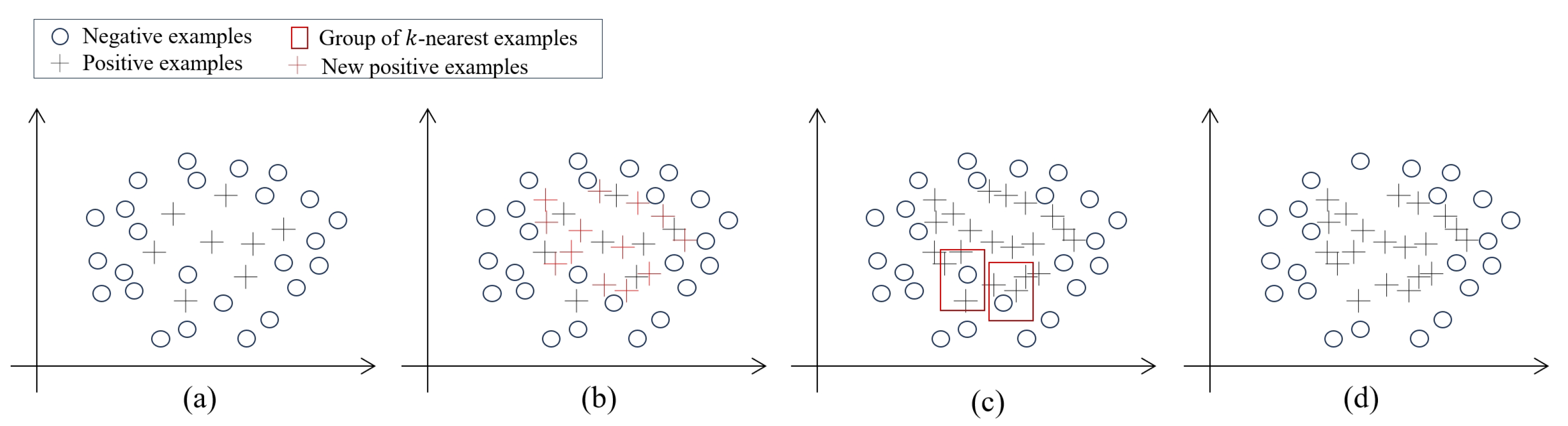
The synthetic minority oversampling technique (SMOTE) [12] is a distance-based method utilized to create synthetic samples within the minority class. Its fundamental principle revolves around the concept that samples sharing the same label within the feature space are considered neighbors. Leveraging the original positions of minority class samples, SMOTE establishes connections between these samples and their neighboring data points, subsequently generating new minority class samples along the connecting lines:

$$x_{new}=x+random(0,1)\times |x-x_n|,$$

(1)

where x is an arbitrary minority class sample, $x_n$ is the nearest neighbor found according to a set sampling ratio n, and $random(0,1)$ is a random factor to prevent repeated adoption.

Adaptive integrated oversampling (ADASYN) [35]. It is similar to SMOTE in that new samples are synthesized through nearest neighbors. The weights of a few classes of samples are added to it. The method is as follows:

• Calculate the total number of new samples to be synthesized:

  $$G=\left(N_{maj}-N_{min}\right)\times random(0,1),$$

  (2)

  where $N_{maj}$ and $N_{min}$ are the samples of majority and minority class, respectively.
• Calculate the weights of the minority class $\widehat{w}$:

  $$\widehat{w}=\frac{w_i}{{\sum }_{i=1}^{N_{min}}{w}_i},w_i=\frac{k_{maj}}{k},$$

  (3)

  where k is the number of nearest neighbors and $k_{maj}$ is the number of majority class samples inside k.
• Calculate the number of new samples that can be synthesized from the majority class samples $g=\widehat{w}\times G$. Generate new samples in the same way as SMOTE.

BorderlineSMOTE [36] represents an enhancement over the conventional SMOTE technique, addressing its limitation of synthesizing minority class samples without regard for data distribution [11]. Specifically, BorderlineSMOTE selects only those minority class samples situated on the decision boundary for synthesis. If the set of boundary points of class p samples is DANGER, and the sample points are $p_1,p_2,\dots p_n$, for each $p_i$, its s nearest neighbors are calculated, and $di{f}_j,j=1,2,\dots s$ is the gap from $p_i$ to its nearest neighbor. Therefore, the new synthesis formula is as follows:

$$x_{new}=p_i+random\left(0,1\right)\times di{f}_j,j=1,2,\dots s$$

(4)

SVMSMOTE [37]. It uses SVM in boundary point decision making for BorderlineSMOTE and is an improved strategy for BorderlineSMOTE. Its synthesis formula is as follows:

$$x_{new}^{+}=s{v}^{+}+\rho (nn\left[i\right]\left[j\right]-s{v}_i^{+}),$$

(5)

where $X_{new}^{+}$ is the newly synthesized positive sample, $s{v}^{+}$ is the set of sample support vectors, $\rho$ is the random number in the range $[0,1]$, $nn$ is an array containing k positive nearest neighbors, and $nn\left[i\right]\left[j\right]$ is the $j_{th}$ positive nearest neighbor of $s{v}^{+}$.

2.2. Undersampling

Cluster centroid [38]. It is a class of undersampling techniques based on the k-means clustering algorithm. Clustering centers $k1, k2, k3,\dots$ are generated by continuous iteration, where $k2$ is the newly generated center after deleting a portion of the majority class samples closest to the center of $k1, k2$, and so on, until the number of positive and negative samples reaches equilibrium. It is not difficult to find that this method requires the majority class samples to be concentrated enough; otherwise, the sampling effect will become worse.

Edited nearest neighbors (ENN) [39]. It is based on the modified k-nearest neighbors rule, which finds the k-nearest neighbors of a certain majority class sample $x_i$, which are $\{x_1,x_2,x_3,\dots x_i,\dots x_n\}$, find the sample points related to it from these nearest neighbors, and remove the misclassified ones, which is an undersampling method. It can achieve the effect of removing the majority class and the minority class samples that are close to each other.

2.3. Combined Resampling

SMOTETomek [40]. It is a combination of SMOTE oversampling and Tomek links [41] of an integrated sampling technique. Tomek links can be formulated in a binary classification task as follows: $x_{maj}$ and $x_{min}$ denote a majority class and a minority class sample, respectively, and $d(x_{maj},x_{min})$ denotes the distance between them. If there is no observation y, which is any $x_{maj}$ or $x_{min}$ such that $d(x_{maj},z)<d(x_{maj},x_{min})$ or $d\left(z,x_{min}\right)<d(x_{maj},x_{min})$, then $d(x_{maj},x_{min})$ is called a Tomek link. Oversampling using SMOTE first and then deleting all the Tomek links can make the decision boundary clearer.

SMOTEENN [42]. It is an integrated sampling technique that combines SMOTE oversampling and ENN undersampling. It resembles SMOTETomek in its approach, both prioritizing the synthesis of minority class samples initially. However, unlike SMOTETomek, it opts not to delete samples in pairs; instead, it selectively removes majority class samples encircled by minority class instances. Due to the requirement for computing neighbors, SMOTEENN carries higher computational costs.

3. Methodology

3.1. Framework and Evaluation Metrics

To explore the performance of various sampling techniques and machine learning models across diverse datasets, we meticulously cleaned, encoded, and feature-screened each dataset, partitioning them into training and test sets, as shown in Figure 1. To maintain consistent prior probabilities, the test and training sets were crafted to possess identical IR as the original dataset [10]. Notably, the test set remained untouched by any balancing techniques to ensure its purity.

The training set underwent RTs via ADASYN (ADA), SMOTE (SMO), BorderlineSMOTE (BSMO), SVMSMOTE (SSMO), cluster centroids (CCs), ENN, SMOTETomek (STOM), and SMOTEENN (SENN), resulting in nine distinct training sets alongside the original unprocessed training set. Each training set was further divided into five validation subsets for cross-validation, facilitating the determination of classifier hyperparameters. Classifiers were categorized into three groups: individual classifiers (logistic regression (LR), k-nearest neighbors (KNN), support vector machine (SVM), naïve Bayes (NB), decision tree (DT)), ensemble classifiers (random forest (RF), XGBoost (XGB), LightGBM (LGBM), CatBoost (CAT)), and balanced classifiers (balanced bagging classifier (BBC), balanced random forest (BRF)). The criterion for selecting classifiers is based on the summary of [43] by reviewing 281 credit-risk-models-related articles (our experiment did not include deep learning algorithms such as artificial neural network [44] and convolutional neural network, although the summary mentioned them, and the reason for their exclusion is their complexity compared with individual classifiers and the higher risk of overfitting they entail; however, their performance does not surpass that of other classifiers [45]). Subsequently, all training sets were subjected to evaluation using these 11 classifiers. We employed the tree-structured Parzen estimator (TPE) for Bayesian optimization to identify optimal hyperparameters and fit the models. Finally, the test set was introduced to the trained classifiers to derive their final evaluation scores. The evaluation metrics comprised as follows:

$$\mathrm{Recall}=\frac{\mathrm{TP}}{\mathrm{TP}+\mathrm{FN}},$$

(6)

$$\mathrm{F}1\mathrm{score}=\frac{2\mathrm{TP}}{2\mathrm{TP}+\mathrm{FP}+\mathrm{FN}},$$

(7)

$$\mathrm{AUC}=\frac{1}{2}(1+\frac{\mathrm{TP}}{\mathrm{TP}+\mathrm{FN}}-\frac{\mathrm{FP}}{\mathrm{FP}+\mathrm{TN}}),$$

(8)

$$\mathrm{Accuracy}=\frac{\mathrm{TP}+\mathrm{TN}}{\mathrm{TP}+\mathrm{FP}+\mathrm{TN}+\mathrm{FN}},$$

(9)

$$\mathrm{G}\text{-}\mathrm{mean}=\sqrt{\mathrm{Recall}\times \mathrm{TNR}},\mathrm{TNR}=\frac{\mathrm{TN}}{\mathrm{TN}+\mathrm{FP}},$$

(10)

while TP, FP, FN, and TN are calculated by

Table 1. Confusion matrix.

		Prediction
		Positive	Negative
Truth	Positive	TP	FN
	Negative	FP	TN

.

Accuracy and recall stand as pivotal metrics in credit risk scenarios, yet their efficacy can be significantly impacted by a CI problem. We retained these metrics to scrutinize the effectiveness of various advanced sampling techniques. Additionally, as previously stated, we assert that minority class samples hold equal importance to majority class samples, and that the ramifications of overlooking a substantial number of good customers mirror those of missing a bad customer. Hence, we also introduce G-means, F1-score, and AUC as evaluation metrics, as suggested in [10,46]. Specifically, AUC will be utilized for subsequent hypothesis testing, as indicated by [10,31].

3.2. Datasets

We chose two benchmark credit datasets, following the recommendation in [10]: the German credit dataset and the Taiwan credit dataset, along with two application-oriented private datasets sourced from Prosper Company and Lending Club Company, as shown in

Table 2. Dataset description.

Source	Data Size	Feature	IR ($\mathit{Majority}/\mathit{Minority}$)
German 1	1000	12	2.33
Taiwan 1	29,995	11	3.52
Prosper 2	113,934	29	4.97
Lending Club (LC) 3	128,400	42	69.24

¹ UCI Machine Learning Repository, https://archive.ics.uci.edu (accessed on 15 September 2023); ² Prosper Company, https://www.prosper.com/credit-card (accessed on 15 September 2023); ³ Lending Club Company, https://www.lendingclub.com (accessed on 15 September 2023).

. These benchmark datasets, extensively utilized in credit risk research over decades, were readily accessible, facilitating the replication of our experiment. In contrast, private datasets, notably those from Lending Club, have gained popularity in the last 5 years due to their richer feature sets and larger data volumes [47], enabling the training of more complex models, each distinct in terms of size, feature dimension, and IR. Notably, the LC dataset stands out as an example of an extremely imbalanced and large dataset. For this dataset, we intend to employ the SH-SENN technique.

3.3. SH-SENN

The process is depicted in the accompanying Figure 2. First, we initiate SMOTE strategic oversampling, wherein minority class samples are sampled to represent 10% to 90% of the majority class. Subsequently, we conduct a search for neighboring samples, which are then removed. Within the 10 new datasets obtained, the ENN proximity strategy is further adjusted to identify new neighboring samples and undergo a subsequent deletion process. Finally, we evaluate the effectiveness of these 10 datasets on the validation set, select the optimal strategy, and apply it to the test set. The key departure from the traditional SMOTEENN lies in our utilization of diverse sampling strategies coupled with cross-verification during the SMOTE process. Moreover, following the initial ENN phase, the dataset undergoes re-evaluation, and adjustments are made to the strategy for selecting the nearest neighbor during the second ENN iteration.

Similar to SENN, SH-SENN also utilizes SMOTE for oversampling, followed by ENN for undersampling. However, there are two significant distinctions between them: First, SENN employs a single ENN undersampling process, whereas SH-SENN utilizes double ENN, meaning ENN is applied again after the regular SENN procedure. Second, while SENN is a mature and combined RT that can be directly applied to any imbalanced dataset, SH-SENN is a framework designed to address imbalance issues. Its approach varies according to the degree of imbalance within datasets. The strategy involves determining the proportion of minority class samples oversampled to majority class samples after the initial SENN step, denoted as $\alpha =N_{nmin}/N_{maj}$, where $N_{nmin}$ represents the number of minority class samples after sampling, and $N_{maj}$ is the number of majority class samples. Typically, $\alpha$ falls within the range of [0.1, 1]. SH-SENN emphasizes treating the strategy as a hyperparameter of the classifier, participating in cross-validation to identify the most suitable $\alpha$ (note: this $\alpha$ is the outcome of the initial ENN participation). Subsequently, after determining the $\alpha$ value, ENN is employed for a second time. This treats the resampled dataset as new data, where ENN undersampling, adept at handling boundary noise, is utilized again to refine the decision boundary. From a technical standpoint, SH-SENN’s primary advantage over SENN lies in its ability to further reduce the introduction of new noise and interference items brought about by SENN. This advantage is particularly evident in extremely imbalanced datasets. These will be validated and presented in subsequent experiments. Lastly, SH-SENN is also an extensible framework; it will be explored in the final section.

3.4. Hypothesis Test

3.4.1. Friedman Test and Nemenyi’s Post Hoc Test

Given that the AUC scores of various RTs across different datasets and classifiers do not adhere to a normal distribution, we employed the Friedman test [48] to assess the hypothesis and determine if there exists a significant difference. Once the null hypothesis is rejected, Nemenyi’s post hoc [48] test is subsequently conducted to delve deeper into the differences between specific pairings.

For n RTs and N observations, the test results of each RT on each observation are ranked from good to bad, and the ordinal values $1,2,3,\dots ,n$ are given. If there is no significant difference in the performance of multiple classifiers, then they are equally divided into ordinal values. Suppose the average ordinal value of the $k$th RTs is $k_i$, then $k_i$ obeys normal distribution and

$${\tau }_{{\chi }^2}=\frac{n-1}{n}\times \frac{12N}{n^2-1}\sum _{i=1}^n\left(k_i-\frac{n+1}{2}\right),$$

(11)

where ${\tau }_{{\chi }^2}$ is chi-square statistic. There is an improved statistic ${\tau }_F$:

$${\tau }_F=\frac{\left(N-1\right){\tau }_{{\chi }^2}}{N\left(n-1\right)-{\tau }_{{\chi }^2}},$$

(12)

where ${\tau }_F$ is subject to the F distribution with a freedom of $n-1$ and $(n-1)(N-1)$.

The difference between the different RTs can then be represented by Nemenyi’s post hoc test, and a Friedman test plot will be generated. If there is no overlapping part of the two-line segments, it means that there is a significant difference between these two classifiers.

3.4.2. Kruskal–Wallis Test and Mann–Whitney U Test

The Kruskal–Wallis test [49] is a nonparametric test used to compare three or more independent samples. It can be used to check whether the results of different datasets and different classifiers come from the same population. It uses the H statistic to test the following:

$$H=\left(\frac{12}{N(N+1)}\sum _{j=1}^k\frac{R_j^2}{n_j}\right)-\mathbf{3}(N+1),$$

(13)

where k is the number of groups, N is the total number of samples, $R_j$ is the rank sum of the jth group, and $n_j$ is the number of samples from each group. If the null hypothesis is rejected, the Mann–Whitney U test [50] is used to perform pair-to-pair grouping tests between small samples that do not satisfy the normal distribution. The result shows whether a particular RT has different scores due to different datasets or different classifiers.

4. Results

4.1. Overall Comparison of RTs

Overall, RTs are significantly different when predicting credit risk, as shown in

Table 3. Friedman test for RTs.

RTs	Median	Statistic	p-Value	Cohen’s f Value
NONE	0.660	58.135	0.000 *** 1	0.126
ADA	0.674
SMO	0.672
BSMO	0.678
SSMO	0.678
CC	0.635
ENN	0.691
STOM	0.680
SENN	0.697

¹ *** represents 1% significance level.

.

Table 4. Post hoc test for RTs.

Pairs	Statistic	p-Value	Cohen’s d Value
NONE vs. ENN	5.092	0.010 ***	0.137
NONE vs. SENN	7.294	0.001 ***	0.175
ADA vs. SENN	5.367	0.005 ***	0.104
SMO vs. SENN	5.505	0.003 ***	0.085
BSMO vs. CC	4.156	0.080 * 1	0.374
BSMO vs. SENN	5.037	0.011 ** 2	0.075
SSMO vs. CC	5.312	0.005 *** 3	0.341
CCvs. ENN	6.991	0.001 ***	0.408
CC vs. STOM	5.312	0.005 ***	0.394
CC vs. SENN	9.193	0.001 ***	0.456

¹ * represents 10% significance level. ² ** represents 5% significance level. ³ *** represents 1% significance level.

shows the pairs’ comparison among RTs with the biggest difference. SENN and ENN emerge as the most effective among all RTs, as shown in Figure 3. Comparatively, when not utilizing any RTs, SENN showcases notable enhancements, boosting AUC, recall, F1-score, and G-mean by up to 20%, 20%, 30%, and 40%, respectively. For instance, in the LC dataset, the G-mean without RTs stands at 0.1168, while after SENN utilization, the G-mean escalates to 0.5715. This demonstrates a notable improvement in both accuracy and recall rates, leading to a more balanced state.

4.2. Comparison of Resampling Techniques in Terms of Different Datasets

In the results for the German dataset (

Table 5. The AUC score of the German dataset by RTs on different classifiers.

Classifiers	Metrics	NONE	ADA	SMO	BSMO	SSMO	CC	ENN	STOM	SENN
LR	AUC	0.6131	0.6512	0.6607	0.6821	0.6679	0.6833	0.6429	0.6607	0.6357
	Recall	0.3333	0.7167	0.7000	0.7500	0.7000	0.7667	0.7500	0.7000	0.8000
	F1	0.4211	0.5342	0.5419	0.5660	0.5490	0.5679	0.5294	0.5419	0.5275
	G-mean	0.5455	0.6479	0.6595	0.6788	0.6671	0.6782	0.6339	0.6595	0.6141
KNN	AUC	0.6179	0.6143	0.6417	0.6357	0.6321	0.6333	0.6274	0.6536	0.6476
	Recall	0.4000	0.6500	0.6833	0.7000	0.6500	0.7167	0.7333	0.7000	0.8667
	F1	0.4486	0.4937	0.5223	0.5185	0.5098	0.5181	0.5146	0.5350	0.5417
	G-mean	0.5782	0.6132	0.6403	0.6325	0.6319	0.6278	0.6184	0.6519	0.6094
SVC	AUC	0.6369	0.6726	0.6560	0.6714	0.6786	0.6702	0.6238	0.6595	0.6655
	Recall	0.3667	0.6167	0.5833	0.6000	0.6500	0.7333	0.7333	0.5833	0.8167
	F1	0.4632	0.5481	0.5263	0.5455	0.5571	0.5535	0.5116	0.5303	0.5537
	G-mean	0.5767	0.6703	0.6519	0.6676	0.6780	0.6673	0.6141	0.6551	0.6481
NB	AUC	0.6524	0.6702	0.6690	0.7012	0.6619	0.7190	0.6595	0.6726	0.6440
	Recall	0.4833	0.7833	0.7667	0.7667	0.7167	0.7667	0.7833	0.7667	0.8167
	F1	0.5088	0.5562	0.5542	0.5860	0.5443	0.6053	0.5465	0.5576	0.5355
	G-mean	0.6300	0.6606	0.6619	0.6981	0.6596	0.7175	0.6478	0.6660	0.6205
DT	AUC	0.5893	0.5619	0.6631	0.6357	0.6012	0.6310	0.6369	0.7000	0.6012
	Recall	0.5000	0.4167	0.6333	0.5500	0.4667	0.7333	0.7667	0.6500	0.5667
	F1	0.4444	0.3968	0.5390	0.5000	0.4480	0.5176	0.5257	0.5821	0.4690
	G-mean	0.5825	0.5428	0.6624	0.6299	0.5859	0.6226	0.6235	0.6982	0.6002
RF	AUC	0.6702	0.6512	0.6690	0.6619	0.6619	0.6952	0.6738	0.6738	0.6690
	Recall	0.4833	0.4667	0.5167	0.5167	0.5167	0.7833	0.7833	0.5333	0.7167
	F1	0.5321	0.5045	0.5344	0.5254	0.5254	0.5802	0.5595	0.5424	0.5513
	G-mean	0.6437	0.6245	0.6515	0.6458	0.6458	0.6896	0.6648	0.6590	0.6674
XGB	AUC	0.6607	0.6429	0.6345	0.6214	0.6321	0.6869	0.7024	0.6381	0.6857
	Recall	0.5000	0.5000	0.4833	0.4500	0.5000	0.8167	0.8334	0.4833	0.7500
	F1	0.5217	0.5000	0.4874	0.4655	0.4878	0.5731	0.5882	0.4915	0.5696
	G-mean	0.6409	0.6268	0.6162	0.5973	0.6182	0.6745	0.6901	0.6190	0.6827
LGBM	AUC	0.6417	0.6833	0.6583	0.6417	0.6357	0.6190	0.6750	0.6560	0.6512
	Recall	0.4333	0.5667	0.5167	0.4833	0.5000	0.7667	0.8000	0.5333	0.7167
	F1	0.4860	0.5574	0.5210	0.4957	0.4918	0.5111	0.5614	0.5203	0.5342
	G-mean	0.6069	0.6733	0.6429	0.6218	0.6211	0.6012	0.6633	0.6444	0.6479
CAT	AUC	0.6964	0.6821	0.6738	0.6929	0.7036	0.7238	0.6833	0.7000	0.6571
	Recall	0.5000	0.5500	0.5333	0.5500	0.6000	0.8333	0.8167	0.5500	0.7500
	F1	0.5714	0.5546	0.5424	0.5690	0.5854	0.6098	0.5698	0.5789	0.5422
	G-mean	0.6682	0.6692	0.6590	0.6780	0.6959	0.7155	0.6702	0.6837	0.6505
BBC	AUC	0.6595	0.6702	0.6167	0.6429	0.6143	0.6714	0.6667	0.6667	0.7024
	Recall	0.5833	0.5333	0.4833	0.4500	0.4500	0.7000	0.7333	0.5333	0.6333
	F1	0.5303	0.5378	0.4677	0.4909	0.4576	0.5526	0.5500	0.5333	0.5846
	G-mean	0.6551	0.6561	0.6021	0.6132	0.5919	0.6708	0.6633	0.6532	0.6990
BRF	AUC	0.7071	0.6524	0.6702	0.6857	0.6583	0.6810	0.6762	0.6821	0.7083
	Recall	0.7500	0.4833	0.5333	0.5500	0.5167	0.7833	0.8167	0.5500	0.7167
	F1	0.5921	0.5088	0.5378	0.5593	0.5210	0.5663	0.5632	0.5546	0.5931
	G-mean	0.7058	0.6301	0.6561	0.6721	0.6429	0.6732	0.6614	0.6692	0.7083

The number in bold in each row indicates the best performance in terms of different metrics.

), it is evident that all RTs, along with the ensemble balanced classifiers BBC and BRF, significantly contribute to the enhancement of the recall score. This indicates a notable improvement in the classifiers’ ability to identify defaulting customers. Particularly noteworthy is the combined effect of CC, which emerges as the top-ranking approach. This can be attributed to the fact that, with an IR of 2.33, the training set still retains 240 minority class samples after undersampling. Consequently, it is sufficiently equipped to handle the test set comprising only 60 minority class samples, thus resulting in a relatively low prediction difficulty. However, according to the Friedman test, no significant difference is observed between several resampling methods. Furthermore, there is no discernible disparity with the NONE dataset.

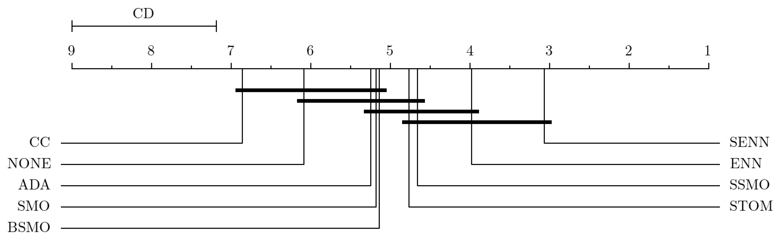
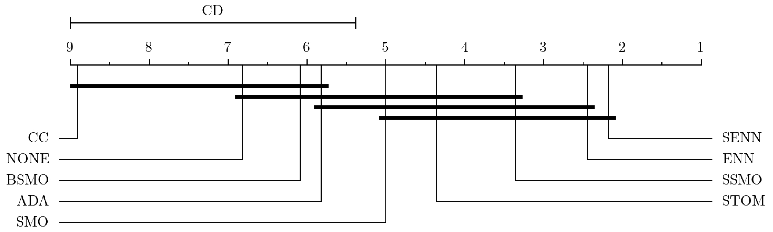
The outcomes obtained from Taiwan (

Table 6. The AUC score of the Taiwan dataset by RTs on different classifiers.

Classifiers	Metrics	NONE	ADA	SMO	BSMO	SSMO	CC	ENN	STOM	SENN
LR	AUC	0.6466	0.7053	0.7021	0.7069	0.7032	0.6131	0.6997	0.7029	0.7064
	Recall	0.3346	0.6029	0.5705	0.6157	0.5629	0.8206	0.5381	0.5727	0.6285
	F1	0.4521	0.5289	0.5292	0.5293	0.5326	0.4194	0.5311	0.5302	0.5263
	G-mean	0.5664	0.6978	0.6896	0.7010	0.6891	0.5769	0.6808	0.6907	0.7021
KNN	AUC	0.6456	0.6419	0.6429	0.6503	0.6576	0.6142	0.6823	0.6456	0.6669
	Recall	0.3677	0.6149	0.5772	0.5968	0.5554	0.8063	0.5901	0.5825	0.6579
	F1	0.4491	0.4423	0.4434	0.4522	0.4626	0.4199	0.4951	0.4467	0.4701
	G-mean	0.5827	0.6413	0.6395	0.6481	0.6496	0.5834	0.6761	0.6425	0.6668
SVC	AUC	0.6580	0.7003	0.7013	0.6995	0.7020	0.6196	0.6999	0.7019	0.7019
	Recall	0.3647	0.6375	0.6066	0.6368	0.6081	0.8365	0.5057	0.6066	0.6338
	F1	0.4747	0.5159	0.5219	0.5148	0.5227	0.4247	0.5383	0.5227	0.5188
	G-mean	0.5890	0.6975	0.6949	0.6967	0.6957	0.5805	0.6724	0.6954	0.6986
NB	AUC	0.6131	0.6961	0.6977	0.6931	0.6976	0.6159	0.7017	0.6993	0.6961
	Recall	0.2683	0.6820	0.6390	0.6722	0.6262	0.8304	0.5365	0.6488	0.6692
	F1	0.3787	0.5047	0.5119	0.5018	0.5134	0.4217	0.5351	0.5130	0.5061
	G-mean	0.5069	0.6959	0.6953	0.6928	0.6940	0.5773	0.6820	0.6975	0.6956
DT	AUC	0.6032	0.6125	0.6162	0.6035	0.6276	0.5861	0.6661	0.6115	0.6701
	Recall	0.3821	0.5207	0.5004	0.4876	0.4951	0.7476	0.6307	0.4951	0.6044
	F1	0.3819	0.4065	0.4095	0.3939	0.4232	0.3962	0.4704	0.4037	0.4770
	G-mean	0.5612	0.6056	0.6052	0.5922	0.6134	0.5634	0.6651	0.6003	0.6669
RF	AUC	0.6544	0.6748	0.6763	0.6745	0.6792	0.6141	0.6973	0.6785	0.6977
	Recall	0.3745	0.5403	0.5185	0.5396	0.5109	0.8093	0.5787	0.5207	0.5893
	F1	0.4664	0.4886	0.4932	0.4882	0.4989	0.4199	0.5198	0.4966	0.5187
	G-mean	0.5915	0.6613	0.6576	0.6609	0.6580	0.5823	0.6872	0.6599	0.6892
XGB	AUC	0.6545	0.6736	0.6768	0.6775	0.6897	0.5992	0.7062	0.6809	0.6971
	Recall	0.3595	0.5546	0.5305	0.5825	0.5456	0.8425	0.5735	0.5335	0.6036
	F1	0.4676	0.4855	0.4927	0.4888	0.5122	0.4100	0.5357	0.4991	0.5158
	G-mean	0.5842	0.6630	0.6608	0.6708	0.6745	0.5476	0.6936	0.6648	0.6908
LGBM	AUC	0.6613	0.6933	0.6973	0.6858	0.7069	0.6127	0.7133	0.7009	0.6986
	Recall	0.3745	0.6142	0.5901	0.6473	0.5870	0.8478	0.5727	0.5916	0.6262
	F1	0.4809	0.5086	0.5180	0.4945	0.5345	0.4198	0.5487	0.5235	0.5149
	G-mean	0.5959	0.6888	0.6890	0.6847	0.6967	0.5658	0.6993	0.6923	0.6948
CAT	AUC	0.6584	0.6841	0.6925	0.6812	0.6952	0.6141	0.7092	0.6907	0.7017
	Recall	0.3677	0.5652	0.5463	0.5916	0.5479	0.8523	0.5690	0.5411	0.6164
	F1	0.4754	0.5005	0.5167	0.4932	0.5211	0.4209	0.5422	0.5145	0.5210
	G-mean	0.5908	0.6737	0.6769	0.6752	0.6794	0.5660	0.6952	0.6743	0.6965
BBC	AUC	0.6778	0.6451	0.6542	0.6480	0.6482	0.6136	0.6900	0.6545	0.6972
	Recall	0.5524	0.4936	0.4913	0.4876	0.4665	0.7679	0.6338	0.4868	0.5780
	F1	0.4921	0.4468	0.4601	0.4510	0.4517	0.4183	0.5015	0.4608	0.5196
	G-mean	0.6661	0.6271	0.6336	0.6278	0.6222	0.5939	0.6877	0.6326	0.6869
BRF	AUC	0.7050	0.6788	0.6771	0.6758	0.6774	0.6129	0.6911	0.6761	0.6962
	Recall	0.6594	0.5456	0.5170	0.5373	0.5064	0.8063	0.6888	0.5177	0.5712
	F1	0.5198	0.4944	0.4948	0.4904	0.4965	0.4189	0.4977	0.4930	0.5192
	G-mean	0.7035	0.6656	0.6579	0.6614	0.6555	0.5816	0.6911	0.6573	0.6849

The number in bold in each row indicates the best performance in terms of different metrics.

) and Prosper (

Table 7. The AUC score of the Prosper dataset by RTs on different classifiers.

Classifiers	Metrics	NONE	ADA	SMO	BSMO	SSMO	CC	ENN	STOM	SENN
LR	AUC	0.9341	0.9468	0.9445	0.9468	0.9423	0.9387	0.9417	0.9447	0.9504
	Recall	0.8692	0.9130	0.8954	0.9030	0.9122	0.8865	0.8886	0.8957	0.9143
	F1	0.9274	0.9089	0.9294	0.9264	0.8903	0.9177	0.9285	0.9295	0.9230
	G-mean	0.9318	0.9462	0.9433	0.9458	0.9418	0.9372	0.9402	0.9434	0.9497
KNN	AUC	0.8223	0.8561	0.8667	0.8655	0.8471	0.8681	0.8434	0.8667	0.8567
	Recall	0.6579	0.8642	0.8435	0.8514	0.7976	0.7924	0.7159	0.8435	0.8710
	F1	0.7631	0.6596	0.7055	0.6949	0.6899	0.7647	0.7696	0.7056	0.6563
	G-mean	0.8057	0.8560	0.8664	0.8654	0.8456	0.8647	0.8337	0.8664	0.8566
SVC	AUC	0.9265	0.9469	0.9447	0.9454	0.9472	0.9422	0.9333	0.9446	0.9447
	Recall	0.8550	0.9072	0.8983	0.9025	0.9135	0.8936	0.8763	0.8983	0.9101
	F1	0.9171	0.9193	0.9248	0.9206	0.9098	0.9214	0.9108	0.9246	0.9044
	G-mean	0.9238	0.9461	0.9436	0.9444	0.9466	0.9409	0.9316	0.9435	0.9441
NB	AUC	0.9422	0.9421	0.9422	0.9418	0.9406	0.9420	0.9441	0.9420	0.9445
	Recall	0.8886	0.8886	0.8889	0.8896	0.8907	0.8847	0.8991	0.8886	0.9043
	F1	0.9309	0.9300	0.9301	0.9268	0.9194	0.9371	0.9208	0.9299	0.9131
	G-mean	0.9407	0.9405	0.9407	0.9403	0.9393	0.9402	0.9431	0.9405	0.9436
DT	AUC	0.9507	0.9527	0.9512	0.9501	0.9490	0.8347	0.9526	0.9514	0.9525
	Recall	0.9190	0.9277	0.9250	0.9245	0.9227	0.9526	0.9250	0.9256	0.9308
	F1	0.9160	0.9101	0.9080	0.9038	0.9021	0.5669	0.9144	0.9079	0.9041
	G-mean	0.9502	0.9524	0.9508	0.9497	0.9486	0.8264	0.9522	0.9510	0.9523
RF	AUC	0.9487	0.9582	0.9558	0.9565	0.9586	0.9032	0.9525	0.9562	0.9600
	Recall	0.8988	0.9242	0.9180	0.9201	0.9250	0.9520	0.9085	0.9193	0.9287
	F1	0.9433	0.9415	0.9418	0.9410	0.9418	0.7114	0.9433	0.9414	0.9417
	G-mean	0.9474	0.9576	0.9551	0.9558	0.9580	0.9018	0.9515	0.9555	0.9594
XGB	AUC	0.9608	0.9604	0.9607	0.9613	0.9634	0.8052	0.9623	0.9611	0.9618
	Recall	0.9245	0.9242	0.9248	0.9261	0.9313	0.9785	0.9287	0.9256	0.9298
	F1	0.9538	0.9519	0.9527	0.9529	0.9536	0.5138	0.9529	0.9530	0.9484
	G-mean	0.9601	0.9597	0.9601	0.9606	0.9629	0.7864	0.9617	0.9604	0.9612
LGBM	AUC	0.9591	0.9615	0.9611	0.9622	0.9625	0.8045	0.9605	0.9614	0.9618
	Recall	0.9206	0.9298	0.9282	0.9308	0.9324	0.9798	0.9253	0.9290	0.9313
	F1	0.9528	0.9471	0.9479	0.9485	0.9473	0.5125	0.9505	0.9482	0.9458
	G-mean	0.9583	0.9610	0.9605	0.9617	0.9621	0.7852	0.9598	0.9609	0.9614
CAT	AUC	0.9581	0.9594	0.9585	0.9606	0.9611	0.8005	0.9593	0.9579	0.9608
	Recall	0.9187	0.9224	0.9203	0.9250	0.9258	0.9785	0.9227	0.9195	0.9271
	F1	0.9514	0.9508	0.9505	0.9519	0.9524	0.5075	0.9497	0.9491	0.9485
	G-mean	0.9573	0.9587	0.9578	0.9600	0.9604	0.7805	0.9586	0.9572	0.9602
BBC	AUC	0.9631	0.9588	0.9562	0.9563	0.9587	0.8796	0.9629	0.9563	0.9586
	Recall	0.9358	0.9242	0.9182	0.9185	0.9245	0.9505	0.9355	0.9187	0.9261
	F1	0.9434	0.9443	0.9431	0.9432	0.9433	0.6552	0.9431	0.9428	0.9400
	G-mean	0.9627	0.9582	0.9554	0.9556	0.9581	0.8768	0.9625	0.9556	0.9580
BRF	AUC	0.9618	0.9577	0.9562	0.9568	0.9585	0.9061	0.9617	0.9567	0.9586
	Recall	0.9368	0.9237	0.9187	0.9201	0.9248	0.9533	0.9368	0.9198	0.9258
	F1	0.9355	0.9401	0.9420	0.9424	0.9422	0.7181	0.9352	0.9426	0.9407
	G-mean	0.9614	0.9571	0.9554	0.9561	0.9579	0.9049	0.9614	0.9560	0.9581

The number in bold in each row indicates the best performance in terms of different metrics.

) underscore a considerable degree of variability among the different RTs. Through Nemenyi’s post hoc tests, we confirm that SENN and ENN emerge as the most effective resampling methods, as Figure 4 and Figure 5 demonstrate. While their efficacy may vary across different classifiers, there is no doubt regarding their applicability across all classifiers. Conversely, CC, which demonstrates dominance in small datasets, ranks last in medium and large datasets. Surprisingly, leaving the dataset untouched (NONE) outperforms the mass removal of most class samples with CC.

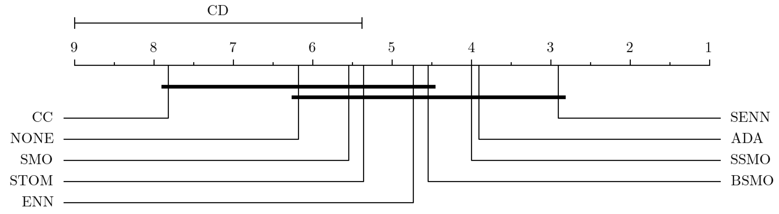
In LC datasets characterized by high IR, there is substantial variability among different resampling methods (

Table 8. The AUC score of the LC dataset by RTs on different classifiers.

Classifiers	Metrics	NONE	ADA	SMO	BSMO	SSMO	CC	ENN	STOM	SENN
LR	AUC	0.5707	0.7766	0.7745	0.7659	0.7615	0.7686	0.5937	0.7745	0.7784
	Recall	0.1421	0.7486	0.7350	0.6284	0.5792	0.8087	0.1885	0.7350	0.7869
	F1	0.2402	0.0981	0.1007	0.1511	0.2117	0.0786	0.2968	0.1007	0.0889
	G-mean	0.3768	0.7761	0.7734	0.7534	0.7393	0.7675	0.4339	0.7734	0.7783
KNN	AUC	0.5065	0.6067	0.6105	0.5879	0.5873	0.5741	0.5275	0.6105	0.6118
	Recall	0.0137	0.3470	0.3525	0.2213	0.2186	0.1831	0.0574	0.3525	0.3934
	F1	0.0258	0.0655	0.0675	0.1014	0.1027	0.1019	0.0940	0.0675	0.0599
	G-mean	0.1168	0.5483	0.5533	0.4596	0.4571	0.4203	0.2393	0.5533	0.5715
SVC	AUC	0.5164	0.6826	0.6887	0.6787	0.7020	0.7313	0.5454	0.6887	0.7021
	Recall	0.0328	0.4262	0.4426	0.3880	0.4344	0.8579	0.0929	0.4426	0.4918
	F1	0.0632	0.1509	0.1488	0.2214	0.2454	0.0588	0.1504	0.1488	0.1302
	G-mean	0.1811	0.6326	0.6433	0.6133	0.6490	0.7203	0.3045	0.6433	0.6699
NB	AUC	0.5000	0.6484	0.6521	0.6455	0.5452	0.6364	0.5000	0.6521	0.6551
	Recall	0.0000	0.5710	0.5683	0.4235	0.0984	0.7104	0.0000	0.5683	0.6175
	F1	0.0000	0.0556	0.0573	0.0800	0.1190	0.0444	0.0000	0.0573	0.0540
	G-mean	0.0000	0.6438	0.6467	0.6061	0.3124	0.6321	0.0000	0.6467	0.6540
DT	AUC	0.6617	0.6213	0.6364	0.6470	0.6387	0.5009	0.6824	0.6364	0.6805
	Recall	0.3361	0.2678	0.2978	0.3142	0.2951	0.9836	0.3798	0.2978	0.4016
	F1	0.3037	0.1782	0.1971	0.2312	0.2338	0.0281	0.3152	0.1971	0.1907
	G-mean	0.5760	0.5109	0.5389	0.5548	0.5384	0.1338	0.6117	0.5389	0.6207
RF	AUC	0.5983	0.5680	0.5748	0.5678	0.5582	0.5005	0.6194	0.5748	0.5872
	Recall	0.1967	0.1366	0.1503	0.1366	0.1175	1.0000	0.2404	0.1503	0.1776
	F1	0.3258	0.2320	0.2506	0.2273	0.1963	0.0281	0.3548	0.2506	0.2539
	G-mean	0.4435	0.3695	0.3875	0.3694	0.3426	0.0327	0.4899	0.3875	0.4207
XGB	AUC	0.6566	0.6485	0.6484	0.6607	0.6617	0.5009	0.6738	0.6484	0.6822
	Recall	0.3142	0.2978	0.2978	0.3224	0.3251	1.0000	0.3497	0.2978	0.3689
	F1	0.4519	0.4395	0.4369	0.4627	0.4508	0.0282	0.4655	0.4369	0.4390
	G-mean	0.5602	0.5455	0.5455	0.5675	0.5697	0.0435	0.5907	0.5455	0.6060
LGBM	AUC	0.6656	0.6405	0.6405	0.6626	0.6680	0.4996	0.6757	0.6405	0.6676
	Recall	0.3333	0.2814	0.2814	0.3279	0.3388	0.9973	0.3552	0.2814	0.3388
	F1	0.4494	0.4301	0.4310	0.4340	0.4436	0.0281	0.4407	0.4310	0.4261
	G-mean	0.5767	0.5304	0.5304	0.5718	0.5813	0.0444	0.5949	0.5304	0.5810
Catboost	AUC	0.6541	0.6527	0.6487	0.6568	0.6539	0.5003	0.6698	0.6487	0.6677
	Recall	0.3087	0.3060	0.2978	0.3142	0.3087	1.0000	0.3415	0.2978	0.3388
	F1	0.4566	0.4562	0.4476	0.4618	0.4484	0.0281	0.4647	0.4476	0.4321
	G-mean	0.5555	0.5530	0.5456	0.5604	0.5554	0.0259	0.5839	0.5456	0.5811
BBC	AUC	0.7641	0.5962	0.6013	0.6354	0.6210	0.5004	0.7798	0.6013	0.6350
	Recall	0.6148	0.1995	0.2104	0.2760	0.2459	0.9836	0.6475	0.2104	0.2814
	F1	0.1618	0.2362	0.2399	0.3378	0.3232	0.0281	0.1676	0.2399	0.2721
	G-mean	0.7494	0.4450	0.4569	0.5240	0.4949	0.1300	0.7685	0.4569	0.5275
BRF	AUC	0.7901	0.5707	0.5680	0.5624	0.5583	0.5006	0.7945	0.5680	0.5929
	Recall	0.7705	0.1421	0.1366	0.1257	0.1175	1.0000	0.7842	0.1366	0.1885
	F1	0.1032	0.2380	0.2309	0.2120	0.1991	0.0281	0.1027	0.2309	0.2738
	G-mean	0.7899	0.3768	0.3695	0.3544	0.3426	0.0344	0.7945	0.3695	0.4336

The number in bold in each row indicates the best performance in terms of different metrics.

). Notably, CC, SMOTE, ADA, and SSMO are found to be ineffective, failing to surpass the performance of NONE (Figure 6). This is particularly evident in terms of F1-score, highlighting the inability of these techniques to enhance model stability and achieve a balanced trade-off between recall and precision. Only SENN emerges as a reliable technique under such circumstances.

Further examination of the relationship between different RTs and datasets can be conducted through the Kruskal–Wallis test (

Table 9. Kruskal–Wallis test for RTs in terms of different datasets.

RTs	Datasets	Median	Statistic	p-Value	Cohen’s f Value
NONE	German	0.652	24.546	0.000 *** 1	0.289
	Taiwan	0.654
	Pros	0.951
	LC	0.654
	Total	0.66
ADA	German	0.652	27.712	0.000 ***	0.302
	Taiwan	0.679
	Pros	0.958
	LC	0.64
	Total	0.674
SMO	German	0.661	28.913	0.000 ***	0.304
	Taiwan	0.677
	Pros	0.956
	LC	0.64
	Total	0.672
BSMO	German	0.662	26.744	0.000 *** 1	0.303
	Taiwan	0.678
	Pros	0.956
	LC	0.647
	Total	0.678
SSMO	German	0.658	27.717	0.000 ***	0.3
	Taiwan	0.69
	Pros	0.958
	LC	0.639
	Total	0.678
CC	German	0.681	31.928	0.000 ***	0.281
	Taiwan	0.614
	Pros	0.88
	LC	0.501
	Total	0.635
ENN	German	0.667	29.498	0.000 ***	0.29
	Taiwan	0.7
	Pros	0.953
	LC	0.67
	Total	0.691
STOM	German	0.667	28.805	0.000 ***	0.304
	Taiwan	0.681
	Pros	0.956
	LC	0.64
	Total	0.68
SENN	German	0.657	28.258	0.000 ***	0.303
	Taiwan	0.697
	Pros	0.959
	LC	0.668
	Total	0.697

¹ *** represents 1% significance level.

). The hypothesis posits that all techniques exhibit significant differences attributable to variations in datasets. For instance, in the case of SENN, its application yields significantly different effects across all subgroups, except for the absence of a significant difference between the German and LC datasets (

Table 10. Pos hoc test for SENN with different datasets.

Two Independent Samples		Statistic	p-Value	Cohen’s d Value
Group A	Group B
SENN-German	SENN-Taiwan	24	0.033 ** 2	1.399
SENN-German	SENN-Pros	0	0.000 *** 3	9.341
SENN-German	SENN-LC	64	1.636	0.015
SENN-Taiwan	SENN-Pros	0	0.000 ***	10.821
SENN-Taiwan	SENN-LC	94	0.056 * 1	0.85
SENN-Pros	SENN-LC	121	0.000 ***	6.496

¹ * represents 10% significance level. ² ** represents 5% significance level. ³ *** represents 1% significance level.

). Moreover, the disparity between Prosper and Taiwan at the 1% significance level suggests that SENN’s efficacy varies depending on the dataset size, while the significant difference between Prosper and LC at the 1% level indicates that SENN’s effectiveness is influenced by the IR of the dataset.

4.3. Comparison of Resampling Techniques in Terms of Different Classifiers

We categorized all classifiers into three groups: individual classifiers, ensemble classifiers, and balanced classifiers. The Kruskal–Wallis test reveals no significant difference between the different types of classifiers except for NONE (

Table 11. Kruskal–Wallis test for RTs in terms of different classifiers.

RTs	Classifier Group	Median	Statistic	p-Value	Cohen’s f Value
NONE	Single	0.641	10.306	0.006 *** 2	0.079
	Ensemble	0.661
	Balanced	0.736
	Total	0.66
ADA	Single	0.678	0.762	0.683	0.014
	Ensemble	0.678
	Balanced	0.661
	Total	0.674
SMO	Single	0.679	0.65	0.722	0.02
	Ensemble	0.675
	Balanced	0.662
	Total	0.672
BSMO	Single	0.688	0.492	0.782	0.012
	Ensemble	0.676
	Balanced	0.662
	Total	0.678
SSMO	Single	0.688	1.446	0.485	0.021
	Ensemble	0.684
	Balanced	0.653
	Total	0.678
CC	Single	0.653	1.857	0.395	0.043
	Ensemble	0.617
	Balanced	0.643
	Total	0.635
ENN	Single	0.674	4.88	0.087 * 1	0.063
	Ensemble	0.7
	Balanced	0.735
	Total	0.691
STOM	Single	0.694	0.304	0.859	0.016
	Ensemble	0.68
	Balanced	0.671
	Total	0.68
SENN	Single	0.688	0.518	0.772	0.008
	Ensemble	0.691
	Balanced	0.7
	Total	0.697

¹ * represents 10% significance level. ² *** represents 1% significance level.

). This suggests that the utilization of RTs can effectively bridge the performance gap between individual and ensemble classifiers, significantly enhancing the effectiveness of weaker classifiers. However, the extent of enhancement provided by different RTs does not exhibit a significant difference.

According to the results of the two independent samples Mann–Whitney U test on grouped variables, the p-value of single classifiers and balanced classifiers on NONE is 0.025 **, indicating statistical significance at the 5% level (

Table 12. Pos hoc test for NONE with classifier groups.

Two Independent Samples		Statistic	p-Value	Cohen’s d Value
Group A	Group B
NONE-Single	NONE-Ensemble	87	0.040 ** 2	0.355
NONE-Single	NONE-Balanced	31	0.025 **	0.692
NONE-Ensemble	NONE-Balanced	30	0.076 * 1	0.361

¹ * represents 10% significance level. ² ** represents 5% significance level.

). This signifies a significant difference between single classifiers and balanced classifiers when no RTs are utilized. The magnitude of the difference, as indicated by a Cohen’s d value of 0.692, falls within the medium range. Conversely, ensemble classifiers and balanced classifiers exhibit a smaller magnitude of difference. This implies that balanced classifiers can effectively address CI problems in the absence of RTs, making them a valuable balancing technique to consider.

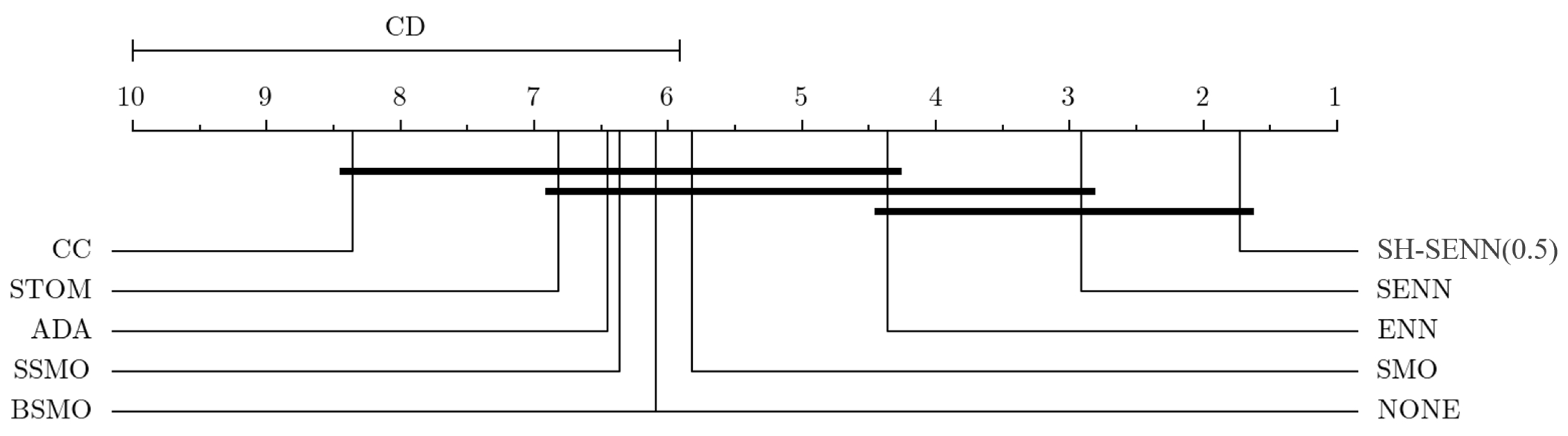
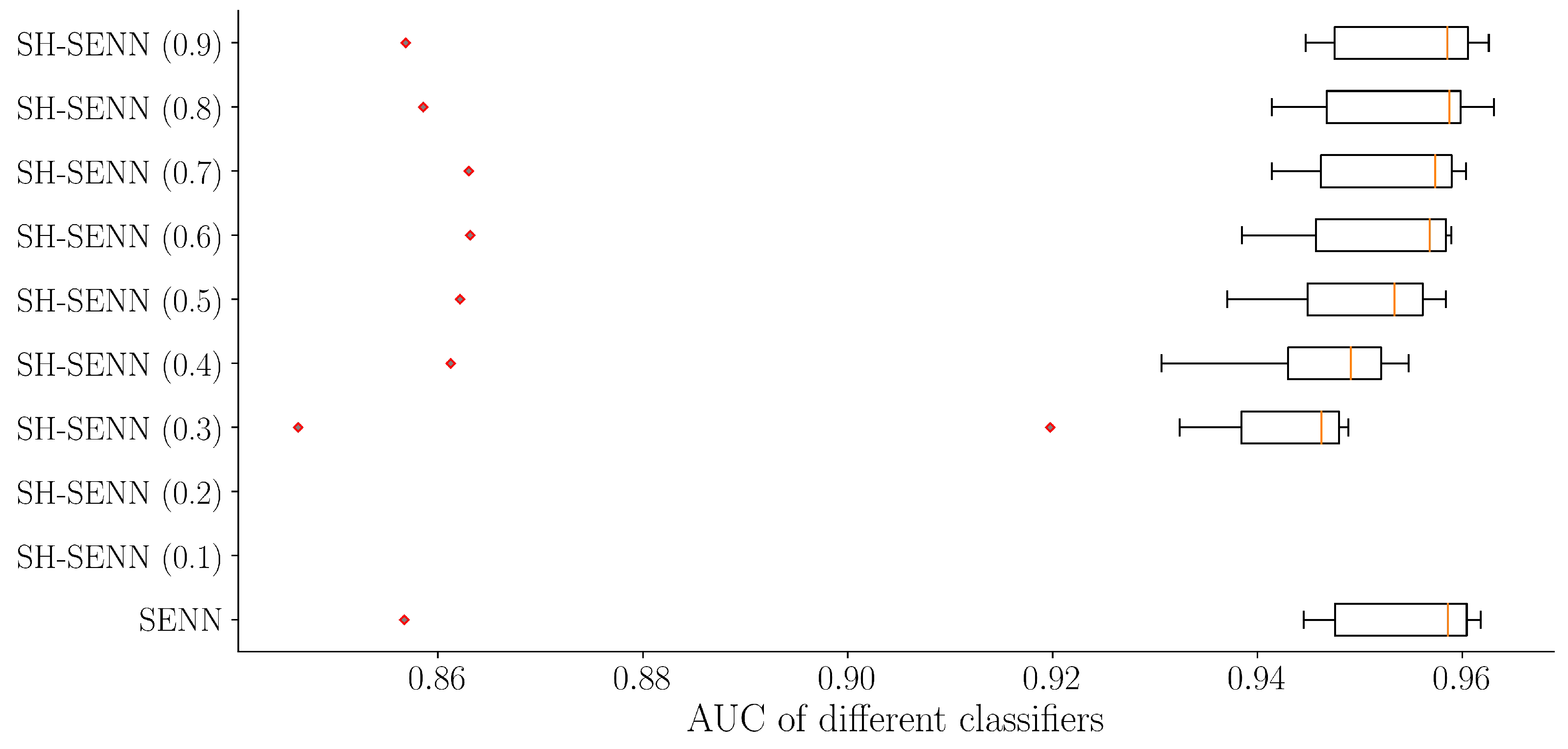
4.4. Experiments with SH-SENN

Significant outcomes were observed with SH-SENN on datasets characterized by high IR (

Table 13. The AUC score of SENN and SH-SENN by different classifiers on the LC dataset.

Classifiers	SENN	SH-SENN (0.1)	SH-SENN (0.2)	SH-SENN (0.3)	SH-SENN (0.4)	SH-SENN (0.5)	SH-SENN (0.6)	SH-SENN (0.7)	SH-SENN (0.8)	SH-SENN (0.9)
LR	0.7784	0.7174	0.7494	0.7651	0.784	0.7848	0.7815	0.7784	0.7768	0.7767
KNN	0.6118	0.59	0.6088	0.5961	0.6126	0.6121	0.6097	0.6052	0.6092	0.6073
SVM	0.7021	0.6701	0.6956	0.7065	0.7071	0.7093	0.7161	0.7136	0.7122	0.6992
NB	0.6551	0.5481	0.5934	0.6161	0.631	0.6545	0.6499	0.6576	0.6573	0.6546
DT	0.6805	0.68	0.6863	0.6745	0.6597	0.6703	0.6604	0.646	0.6829	0.6329
RF	0.5872	0.6237	0.6398	0.6301	0.6302	0.6315	0.617	0.6165	0.6021	0.5984
XGB	0.6822	0.6863	0.6834	0.6874	0.6861	0.6956	0.6889	0.6833	0.6833	0.6824
LGBM	0.6676	0.6808	0.6768	0.6714	0.6754	0.6783	0.6742	0.6671	0.6781	0.6703
CAT	0.6677	0.685	0.6823	0.685	0.685	0.6797	0.6852	0.6825	0.6797	0.6745
BBC	0.635	0.7169	0.7270	0.703	0.6933	0.6917	0.6777	0.6811	0.6739	0.6358
BRF	0.5929	0.7194	0.6916	0.6617	0.6355	0.6308	0.6112	0.6139	0.606	0.5996

The number in bold in each row indicates the best performance in terms of different metrics.

). Irrespective of the strategy ratio $\alpha$ employed, SH-SENN consistently enhances the prediction performance of ensemble classifiers and balanced classifiers. This enhancement reaches its peak when $\alpha$ approaches 0.5, followed by a diminishing trend. However, for individual classifiers, SH-SENN proves to be less effective than SENN when $\alpha$ is below 0.4. Notably, SH-SENN outperforms SENN when $\alpha$ falls between 0.4 and 0.7. Overall, the results highlight SH-SENN (0.5) as the most advantageous and effective new RT, as shown in Figure 7.

The Friedman test results reveal that SH-SENN exhibits varying degrees of significant differences and advantages over NONE, ADA, SMO, BSMO, SSMO, CC, and STOM (

Table 14. Pos hoc test for SH-SENN with RTs on the LC dataset.

Pairs	Statistic	p-Value	Cohen’s d Value
NONE vs. SH-SENN (0.5)	4.97	0.046 ** 2	0.654
ADA vs. SH-SENN (0.4)	5.027	0.040 **	0.66
ADA vs. SH-SENN (0.5)	5.789	0.005 *** 3	0.731
ADA vs. SH-SENN (0.6)	4.857	0.060 * 1	0.598
SMO vs. SH-SENN (0.5)	5.281	0.022 **	0.686
BSMO vs. SH-SENN (0.4)	4.801	0.068 *	0.568
BSMO vs. SH-SENN (0.5)	5.563	0.010 **	0.639
BSMO vs. SH-SENN (0.6)	4.631	0.096 *	0.508
SSMO vs. SH-SENN (0.4)	5.14	0.031 **	0.693
SSMO vs. SH-SENN (0.5)	5.902	0.004 ***	0.758
SSMO vs. SH-SENN (0.6)	4.97	0.046 **	0.637
SSMO vs. SH-SENN (0.8)	4.688	0.086 *	0.618
CC vs. SH-SENN (0.2)	5.196	0.027 **	1.404
CC vs. SH-SENN (0.3)	4.857	0.060 *	1.358
CC vs. SH-SENN (0.4)	5.93	0.004 ***	1.356
CC vs. SH-SENN (0.5)	6.693	0.001 ***	1.405
CC vs. SH-SENN (0.6)	5.761	0.006 ***	1.311
CC vs. SH-SENN (0.7)	4.801	0.068 *	1.284
CC vs. SH-SENN (0.8)	5.478	0.013 **	1.296
STOM vs. SH-SENN (0.5)	5.281	0.022 **	0.686

¹ * represents 10% significance level. ² ** represents 5% significance level. ³ *** represents 1% significance level.

). Notably, the AUC can reach a maximum of 0.784. Post hoc tests confirm that although there is no significant difference between SH-SENN (0.5) and the previous champion SENN (Figure 8), it still secures the top rank among all RTs with a substantial advantage.

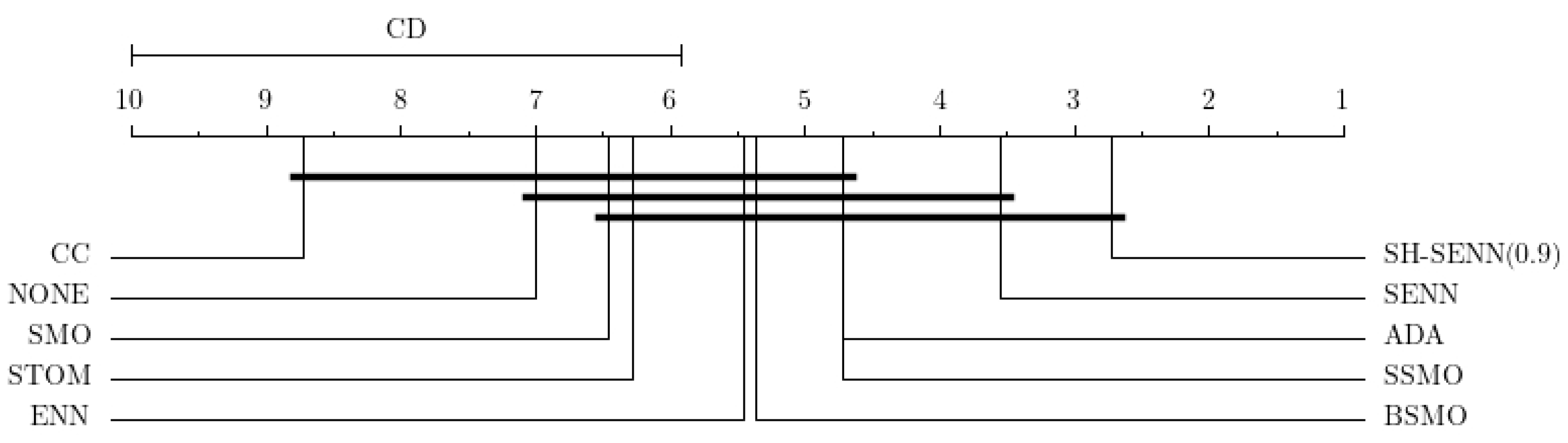
Under various IR conditions, we included the Prosper dataset in the experiment to compare the performance of SH-SENN. This dataset shares the same size as the LC dataset and has an IR of 4.97, representing a normal imbalanced dataset. With positive samples comprising more than 20% of negative samples in the Prosper dataset’s training set, the strategy ratio $\alpha$ for this round ranged from 0.3 to 0.9 (if $\alpha$ was less than 0.2, undersampling will be conducted initially; however, SMOTE as the first step for SH-SENN is an oversampling method).

Results were compared with SENN, which ranked first on the Prosper dataset in a previous result. The findings reveal that (

Table 15. The AUC score of SENN and SH-SENN by different classifiers on the Prosper dataset.

Classifiers	SENN	SH-SENN (0.3)	SH-SENN (0.4)	SH-SENN (0.5)	SH-SENN (0.6)	SH-SENN (0.7)	SH-SENN (0.8)	SH-SENN (0.9)
LR	0.9504	0.9324	0.9410	0.9447	0.9464	0.9476	0.9492	0.9503
KNN	0.8567	0.8464	0.8612	0.8621	0.8631	0.8630	0.8585	0.8568
SVM	0.9447	0.9198	0.9306	0.9370	0.9385	0.9414	0.9414	0.9448
NB	0.9445	0.9444	0.9449	0.9450	0.9450	0.9448	0.9443	0.9447
DT	0.9525	0.9486	0.9517	0.9531	0.9532	0.9542	0.9528	0.9515
RF	0.9600	0.9458	0.9483	0.9544	0.9570	0.9583	0.9598	0.9587
XGB	0.9618	0.9469	0.9524	0.9565	0.9589	0.9604	0.9631	0.9626
LGB	0.9618	0.9473	0.9514	0.9557	0.9581	0.9602	0.9611	0.9623
CAT	0.9608	0.9462	0.9491	0.9534	0.9568	0.9583	0.9598	0.9612
BBC	0.9586	0.9487	0.9527	0.9576	0.9587	0.9574	0.9587	0.9599
BRF	0.9586	0.9489	0.9547	0.9584	0.9589	0.9596	0.9592	0.9585

The number in bold in each row indicates the best performance in terms of different metrics.

), under the interference of SH-SENN, all classifiers except LR and RF achieved higher AUC values. This suggests that SH-SENN can outperform SENN even in normal IR datasets, albeit with a smaller improvement compared with extreme IR datasets.

A significant difference from the results in the LC dataset was that the SH-SENN (0.9) strategy yielded the best results, contrary to the previous SH-SENN (0.5) strategy. The average AUC of SH-SENN (0.9) across all classifiers reached 0.9465, slightly higher than SENN’s average AUC of 0.9464 (Figure 9). This discrepancy arises because minority samples in normally imbalanced datasets contain more information than extremely imbalanced minority samples, and there is less noise when oversampling to 90% of the majority sample. Experiments demonstrate that the strategy ratio of SH-SENN should decrease with an increasing IR to achieve better results.

Similarly, the Friedman test results indicate significant differences between SH-SENN (0.9) and NONE, ADA, SMO, BSMO, SSMO, CC, and STOM in the Prosper dataset. Subsequent post hoc tests revealed that SH-SENN (0.9) surpassed all other RTs by a considerable margin (Figure 10). These two sets of experiments collectively demonstrate that SH-SENN can achieve comparable effectiveness to other RTs across various IR datasets, albeit requiring different strategy ratios (

Table 16. Pos hoc test for SH-SENN with RTs on the Prosper dataset.

Pairs	Statistic	p-Value	Cohen’s d Value
ADA vs. SH-SENN (0.3)	5.098	0.028 ** 2	0.374
BSMO vs. SH-SENN (0.3)	4.686	0.071 * 1	0.401
SSMO vs. SH-SENN (0.3)	5.13	0.026 **	0.324
CC vs. SH-SENN (0.7)	4.845	0.050 *	1.588
CC vs. SH-SENN (0.8)	5.605	0.007 *** 3	1.575
CC vs. SH-SENN (0.9)	6.301	0.001 ***	1.575
SENN vs. SH-SENN (0.3)	6.365	0.001 ***	0.403
SENN vs. SH-SENN (0.4)	4.591	0.087 *	0.229

¹ * represents 10% significance level. ² ** represents 5% significance level. ³ *** represents 1% significance level.

). Moreover, the impact of SH-SENN on classifier enhancement is more pronounced in high IR datasets compared with those with common IR levels.

4.5. Discussion and Limitation

Overall, the experimental results align with our discussion in Section 2. We contend that the CI problem does not directly impact the classifier’s predictive ability but rather obscures the decision boundary, thereby weakening its performance. Certain RTs, such as SMOTE, ADASYN, and cluster centroids, address the CI problem by either oversampling or undersampling to bring the classes closer to equilibrium. However, they merely generate new minority class samples or remove majority class samples without specifically optimizing the decision boundary or addressing the issue of overlapping samples from different classes. Consequently, these techniques prove ineffective across various datasets. SVMSMOTE and BorderlineSMOTE achieve superior results because they focus on generating minority class samples along the border, thereby enhancing the clarity of the decision boundary. Moreover, in SMOTEENN, the ENN method supplements the limitations of the SMOTE-only oversampling approach, which tends to marginalize data distribution. Unlike SMOTETomek, which combines oversampling and undersampling but removes entire pairs, SMOTEENN selectively eliminates examples that do not align with neighboring categorizations. As a result, ENN preserves more information than Tomek link, rendering SMOTEENN more stable and effective across diverse datasets. While SMOTETomek excels in datasets with a pronounced class overlap, it may yield better results in credit datasets characterized by higher feature dimensions and greater diversity in types.

From the dataset perspective, small datasets characterized by limited sample sizes, data structures, and small training sets exhibit no significant disparities among different resampling RTs. Even with oversampling, the potential for expanding the dataset’s information content remains limited. Conversely, medium and large datasets demonstrate similarities in their RT selection. This can be attributed to the classifiers’ capacity to learn sufficient predictive information when the training set is relatively ample. However, further improvement in prediction ability necessitates optimizing decision boundaries in addition to resampling, making combined sampling more effective. On the contrary, large datasets with a high IR demand cautious treatment. These datasets feature high-dimensional features, complex data structures, and sparse minority class samples. Consequently, classifiers may struggle to recognize positive samples unseen during training, resulting in low recall scores. Oversampling the minority class to excessively high proportions, such as with a SMOTE ratio of 1:1 or 1:0.9, may lead to an accumulation of minority class samples without clarifying the decision boundary, potentially generating new noise. In such scenarios, random oversampling may outperform SMOTE [30]. To address extreme CI, it is advisable to employ a smaller ratio oversampling strategy to prevent an abundance of minority class samples from becoming noise. Emphasizing the handling of boundary points and class overlapping is crucial. SH-SENN stands out as a superior technique due to its strategic oversampling approach and dual handling of boundary points, which contribute to achieving better results compared with other RTs.

From the classifier’s standpoint, ensemble classifiers tend to benefit more from RTs compared with individual classifiers due to their enhanced learning capabilities. This is particularly evident in the boosting family of classifiers, such as XGBoost. When employing oversampling or integrated sampling RTs, the ensemble classifier can capitalize on the increased effective information within the dataset, thereby maximizing its predictive performance. Conversely, when using RTs like cluster centroids, which drastically reduce the amount of information, the ensemble classifier’s performance remains robust, and even regular individual classifiers can achieve satisfactory results. While ensemble classifiers offer hyperparameters to adjust category weights, predicting these weights for a few sample categories in real-world scenarios is impractical. Furthermore, presetting these weights is not feasible, considering the test set’s consistent IR with the training set in this study to ensure comparable effects of different RTs and avoid inconsistent prediction difficulty in the test set. For instance, suppose a bank encounters 10 defaulting credit customers monthly, with the bank approving 10 applicants daily. These defaulters may be distributed over 30 days or concentrated on a single day. Processing the training set beforehand allows for the construction of a robust classifier prior to model fitting.

Lastly, concerning the credit risk prediction problem, real credit data often exhibit high feature dimensions and diverse data types. Existing studies frequently concentrate solely on comparing balancing methods and integrating them with classification models, overlooking the practical significance of aiding credit institutions in addressing the CI problem. Their findings tend to be purely theoretical and algorithmic, failing to address the core issue. For instance, clustering-based undersampling may perform well only with specific datasets and models. If a credit institution modifies user profiles, incorporates new features, or includes audio and video features, the original sampling approach may no longer be suitable for the updated dataset. Thus, applicability becomes a concern. The SH-SENN sampling technique proposed in this study is not a rigid algorithm but rather a versatile framework. The undersampling technique within this framework is ENN, but it can be substituted with other undersampling methods to create new algorithms while remaining within the framework’s conceptual scope. Additionally, SH-SENN employs the more representative Lending Club dataset for experimentation and achieves promising results. This illustrates the framework’s potential for extension to analogous credit datasets and its applicability to classification tasks facing CI challenges. For instance, food safety regulation represents a critical concern in Africa, where establishing an early warning system to oversee food quality is imperative. Given the high stakes involved in safeguarding human life, the testing of positive samples becomes more exacting, necessitating robust and balanced datasets for constructing monitoring models. Even a marginal enhancement in model performance achieved by methods like SH-SENN could potentially safeguard the health of numerous individuals. Similar applications can also be extrapolated to medical disease detection and the machinery industry.

SH-SENN also possesses potential limitations. In comparison with other RTs, SH-SENN requires a longer time for resampling due to its utilization of double ENN. This extended duration arises from the necessity for both SMOTE and ENN to formulate their neighbors to facilitate distance-based computations. Consequently, this process consumes more time, particularly in large datasets with high-dimensional features. Moreover, our experiments did not explore the compatibility of SH-SENN with deep learning algorithms such as artificial neural networks. As previously mentioned, deep learning algorithms currently do not offer significant advantages in credit risk prediction but will be questioned by stakeholders because of its black-box property. Nonetheless, deep learning undoubtedly represents a crucial avenue for future research. We expect that combining SH-SENN with deep learning algorithms will yield superior results.

5. Conclusions

We conducted a comprehensive comparison and analysis of various RTs in the experiment, introducing a novel RT tailored for extremely imbalanced datasets. The conclusion can be summarized as follows:

• SMOTEENN significantly enhances dataset quality before classifier training, consistently improving prediction performance across all selected credit datasets. Compared with the original training set without SMOTEENN preprocessing, AUC values see an increase of 2–4%, and recall values show enhancements of up to 30%. The effectiveness of RTs varies significantly depending on dataset size and IR. For small-sized datasets with a low IR, the choice of RT does not yield significant differences. However, for medium and large-sized datasets with varying IRs, RTs capable of managing decision boundaries and class coincidence points yield superior results. Notably, SMOTEENN stands out in this regard. RTs particularly boost ensemble classifiers over single classifiers. Balanced ensemble classifiers can perform reasonably well without preprocessing RTs, although their predictive power is not as stable as classifiers with RTs applied in advance. Moreover, the choice of classifiers for credit approval should consider interpretability, as high-performance ensemble classifiers may lack interpretability, posing challenges for acceptance by stakeholders. Thus, classifiers like logistic regression and decision trees, known for their interpretability and fast execution, remain widely used despite their potentially poorer performance. Computational cost and interpretability should be key factors when selecting RTs.
• For SH-SENN, first, the new SH-SENN demonstrates outstanding performance in handling extremely imbalanced large datasets. This is attributed to its focus on addressing decision boundary points and noise points after oversampling. In real-world scenarios, credit data are often intricate, featuring time-varying attributes and numerous sparse categorical variables. Datasets exhibiting high IR and significant noise, such as those from Lending Club Inc., are commonplace. SH-SENN emerges as the optimal solution meeting these realistic requirements. Second, as credit datasets grow increasingly complex, there arises a need for high-performing classifiers to replace traditional scorecard and logistic regression (LR) algorithms. Emerging classifiers like CatBoost prove to be suitable candidates for credit datasets owing to their improved handling of categorical variables. However, they still fall short in effectively addressing CI concerns alone. CatBoost also requires complementary techniques to enhance its efficacy. Our experiments demonstrate that SH-SENN significantly enhances the predictive capabilities of ensemble classifiers compared with individual classifiers. SH-SENN outperforms all other strategies ranging from 0.1 to 0.9, including established techniques like SMOTEENN. This enhancement results in a 1–5% improvement in AUC for various classifiers. Notably, the improvement for CatBoost alone can nearly reach 2%. Such enhancements are highly appealing for credit bureaus, where even a 1% improvement can potentially help them avoid millions of dollars in losses.

In light of our research, future directions include employing additional model evaluation metrics for comprehensive comparisons, exploring relationships between IR and RTs using simulated datasets, and investigating RT combinations tailored for high-performance ensemble classifiers.

References

1. Henley, W.; Hand, D.J. A k-nearest-neighbour classifier for assessing consumer credit risk. J. R. Stat. Soc. 1996, 45, 77–95. [Google Scholar] [CrossRef]
2. Abellán, J.; Castellano, J.G. A comparative study on base classifiers in ensemble methods for credit scoring. Expert Syst. Appl. 2017, 73, 1–10. [Google Scholar] [CrossRef]
3. Tsai, C.F.; Wu, J.W. Using neural network ensembles for bankruptcy prediction and credit scoring. Expert Syst. Appl. 2008, 34, 2639–2649. [Google Scholar] [CrossRef]
4. Andrés Alonso, J.M.C. Machine Learning in Credit Risk: Measuring the Dilemma between Prediction and Supervisory Cost; Banco de España: Madrid, Spain, 2020. [Google Scholar]
5. Ding, S.; Cui, T.; Bellotti, A.; Abedin, M.; Lucey, B. The role of feature importance in predicting corporate financial distress in pre and post COVID periods: Evidence from China. Int. Rev. Financ. Anal. 2023, 90, 102851. [Google Scholar] [CrossRef]
6. Wang, L. Imbalanced credit risk prediction based on SMOTE and multi-kernel FCM improved by particle swarm optimization. Appl. Soft Comput. 2022, 114, 108153. [Google Scholar] [CrossRef]
7. Moscato, V.; Picariello, A.; Sperlí, G. A benchmark of machine learning approaches for credit score prediction. Expert Syst. Appl. 2021, 165, 113986. [Google Scholar] [CrossRef]
8. García, V.; Marqués, A.I.; Sánchez, J.S. Exploring the synergetic effects of sample types on the performance of ensembles for credit risk and corporate bankruptcy prediction. Inf. Fusion 2019, 47, 88–101. [Google Scholar] [CrossRef]
9. Haixiang, G.; Li, Y.; Shang, J.; Mingyun, G.; Yuanyue, H.; Gong, B. Learning from class-imbalanced data: Review of methods and applications. Expert Syst. Appl. 2016, 73, 220–239. [Google Scholar] [CrossRef]
10. García, V.; Marqués, A.I.; Sánchez, J.S. An insight into the experimental design for credit risk and corporate bankruptcy prediction systems. J. Intell. Inf. Syst. 2015, 44, 159–189. [Google Scholar] [CrossRef]
11. Niu, K.; Zhang, Z.; Liu, Y.; Li, R. Resampling ensemble model based on data distribution for imbalanced credit risk evaluation in P2P lending. Inf. Sci. 2020, 536, 120–134. [Google Scholar] [CrossRef]
12. Chawla, N.V.; Bowyer, K.W.; Hall, L.O.; Kegelmeyer, W.P. SMOTE: Synthetic minority over-sampling technique. Artif. Intell. 2002, 16, 321–357. [Google Scholar] [CrossRef]
13. Cui, T.; Li, J.; John, W.; Andrew, P. An ensemble based Genetic Programming system to predict English football premier league games. In Proceedings of the 2013 IEEE Symposium Series on Computational Intelligence (SSCI2013), Singapore, 16–19 April 2013; pp. 138–143. [Google Scholar] [CrossRef]
14. Fiore, U.; De Santis, A.; Perla, F.; Zanetti, P.; Palmieri, F. Using generative adversarial networks for improving classification effectiveness in credit card fraud detection. Inf. Sci. 2019, 479, 448–455. [Google Scholar] [CrossRef]
15. Jiang, C.; Lu, W.; Wang, Z.; Ding, Y. Benchmarking state-of-the-art imbalanced data learning approaches for credit scoring. Expert Syst. Appl. 2023, 213, 118878. [Google Scholar] [CrossRef]
16. Ding, S.; Cui, T.; Zhang, Y. Incorporating the RMB internationalization effect into its exchange rate volatility forecasting. N. Am. J. Econ. Financ. 2020, 54, 101103. [Google Scholar] [CrossRef]
17. Ding, S.; Cui, T.; Zheng, D.; Du, M. The effects of commodity financialization on commodity market volatility. Resour. Policy. 2021, 73, 102220. [Google Scholar] [CrossRef]
18. Zhu, R.; Guo, Y.; Xue, J.H. Adjusting the imbalance ratio by the dimensionality of imbalanced data. Pattern Recognit. Lett. 2020, 133, 217–223. [Google Scholar] [CrossRef]
19. Dorogush, A.V.; Ershov, V.; Gulin, A. CatBoost: Gradient boosting with categorical features support. arXiv 2018, arXiv:1810.11363. [Google Scholar]
20. Ke, G.; Meng, Q.; Finley, T.; Wang, T.; Chen, W.; Ma, W.; Ye, Q.; Liu, T.Y. LightGBM: A highly efficient gradient boosting decision tree. In Proceedings of the 31st International Conference on Neural Information Processing Systems, Red Hook, NY, USA, 4–9 December 2017; pp. 3149–3157. [Google Scholar]
21. Caouette, J.; Altman, E.; Narayanan, P.; Nimmo, R. Managing Credit Risk: The Great Challenge for the Global Financial Markets, 2nd ed.; John Wiley & Sons: Hoboken, NJ, USA, 2011; pp. 349–365. [Google Scholar] [CrossRef]
22. Khan, A.A.; Chaudhari, O.; Chandra, R. A review of ensemble learning and data augmentation models for class imbalanced problems: Combination, implementation and evaluation. Expert Syst. Appl. 2024, 244, 122778. [Google Scholar] [CrossRef]
23. Xia, Y.; Liu, C.; Liu, N. Cost-sensitive boosted tree for loan evaluation in peer-to-peer lending, Electron. Commer. Res. Appl 2017, 24, 30–49. [Google Scholar]
24. Liu, X.Y.; Wu, J.; Zhou, Z.H. Exploratory undersampling for class-Imbalance learning. IEEE Trans. Syst. Man Cybern. Part B 2009, 39, 539–550. [Google Scholar] [CrossRef]
25. Liu, B.; Chen, K. Loan risk prediction method based on SMOTE and XGBoost. Comput. Mod. 2020, 2, 26–30. [Google Scholar]
26. Zięba, M.; Tomczak, J.M. Boosted SVM with active learning strategy for imbalanced data. Soft Comput. 2015, 19, 3357–3368. [Google Scholar] [CrossRef]
27. Ding, S.; Cui, T.; Wu, X.; Du, M. Supply chain management based on volatility clustering: The effect of CBDC volatility. Res. Int. Bus. Financ. 2022, 62, 101690. [Google Scholar] [CrossRef]
28. Yen, S.J.; Lee, Y.S. Cluster-based under-sampling approaches for imbalanced data distributions. Expert Syst. Appl. 2009, 36, 5718–5727. [Google Scholar] [CrossRef]
29. García, V.; Marqués, A.I.; Sánchez, J.S. Improving Risk Predictions by Preprocessing Imbalanced Credit Data. In Neural Information Processing; Huang, T., Zeng, Z., Li, C., Leung, C.S., Eds.; Springer: Berlin/Heidelberg, Germany, 2012; pp. 68–75. [Google Scholar]
30. Xiao, J.; Wang, Y.; Chen, J.; Xie, L.; Huang, J. Impact of resampling methods and classification models on the imbalanced credit scoring problems. Inf. Sci. 2021, 569, 508–526. [Google Scholar] [CrossRef]
31. Brown, I.; Mues, C. An experimental comparison of classification algorithms for imbalanced credit scoring data sets. Expert Syst. Appl. 2012, 39, 3446–3453. [Google Scholar] [CrossRef]
32. Chen, T.; Guestrin, C. XGBoost: A scalable tree boosting system. In Proceedings of the 22nd ACM SIGKDD International Conference on Knowledge Discovery and Data Mining, San Francisco, CA, USA, 13–17 August 2016. [Google Scholar]
33. Ma, X.; Sha, J.; Wang, D.; Yu, Y.; Yang, Q.; Niu, X. Study on a prediction of P2P network loan default based on the machine learning LightGBM and XGboost algorithms according to different high dimensional data cleaning. Electron. Commer. Res. Appl. 2018, 31, 24–39. [Google Scholar] [CrossRef]
34. Kou, G.; Chen, H.; Hefni, M.A. Improved hybrid resampling and ensemble model for imbalance learning and credit evaluation. J. Manag. Sci. Eng. 2022, 7, 511–529. [Google Scholar] [CrossRef]
35. Haibo, H.; Yang, B.; Garcia, E.A.; Shutao, L. ADASYN: Adaptive synthetic sampling approach for imbalanced learning. In Proceedings of the 2008 IEEE International Joint Conference on Neural Networks (IEEE World Congress on Computational Intelligence), Hong Kong, 1–8 June 2008; pp. 1322–1328. [Google Scholar] [CrossRef]
36. Han, H.; Wang, W.Y.; Mao, B.H. Borderline-SMOTE: A New Over-Sampling Method in Imbalanced Data Sets Learning. In Advances in Intelligent Computing; Huang, D.S., Zhang, X.P., Huang, G.B., Eds.; Springer: Berlin/Heidelberg, Germany, 2005; pp. 878–887. [Google Scholar]
37. Nguyen, H.M.; Cooper, E.W.; Kamei, K. Borderline over-sampling for imbalanced data classification. Int. J. Knowl. Eng. Soft Data Paradig. 2009, 3, 4–21. [Google Scholar] [CrossRef]
38. Han, J.; Kamber, M.; Pei, J. (Eds.) 3—Data Preprocessing. In Data Mining, 3rd ed.; Morgan Kaufmann: Boston, MA, USA, 2012; pp. 83–124. [Google Scholar] [CrossRef]
39. Wilson, D.L. Asymptotic Properties of Nearest Neighbor Rules Using Edited Data. IEEE Trans. Syst. Man Cybern. 1972, SMC-2, 408–421. [Google Scholar] [CrossRef]
40. Batista, G.E.A.P.A.; Bazzan, A.L.C.; Monard, M.C. Balancing Training Data for Automated Annotation of Keywords: A Case Study. WOB 2003, 3, 1–9. [Google Scholar]
41. Tomek, I. Two Modifications of CNN. IEEE Trans. Syst. Man Cybern. 1976, SMC-6, 769–772. [Google Scholar] [CrossRef]
42. Batista, G.E.A.P.A.; Prati, R.C.; Monard, M.C. A study of the behavior of several methods for balancing machine learning training data. ACM SIGKDD Explor. Newsl. 2004, 6, 20–29. [Google Scholar] [CrossRef]
43. Zhang, X.; Yu, L. Consumer credit risk assessment: A review from the state-of-the-art classification algorithms, data traits, and learning methods. Expert Syst. Appl. 2024, 237, 121484. [Google Scholar] [CrossRef]
44. Chai, E.; Wei, Y.; Cui, T.; Ren, J.; Ding, S. An Efficient Asymmetric Nonlinear Activation Function for Deep Neural Networks. Symmetry 2022, 14, 1027. [Google Scholar] [CrossRef]
45. Dastile, X.; Celik, T.; Potsane, M. Statistical and machine learning models in credit scoring: A systematic literature survey. Appl. Soft Comput. 2020, 91, 106263. [Google Scholar] [CrossRef]
46. Ferri, C.; Hernández-Orallo, J.; Modroiu, R. An experimental comparison of performance measures for classification. Pattern Recognit. Lett. 2009, 30, 27–38. [Google Scholar] [CrossRef]
47. Markov, A.; Seleznyova, Z.; Lapshin, V. Credit scoring methods: Latest trends and points to consider. J. Financ. Data Sci. 2022, 8, 180–201. [Google Scholar] [CrossRef]
48. Pereira, D.; Afonso, A.; Medeiros, F. Overview of Friedman’s Test and Post-hoc Analysis. Commun. Stat.-Simul. Comput. 2015, 44, 2636–2653. [Google Scholar] [CrossRef]
49. McKight, P.E.; Najab, J. Kruskal-Wallis Test. In The Concise Encyclopedia of Statistics; Springer: New York, NY, USA, 2008; pp. 288–290. [Google Scholar] [CrossRef]
50. Meléndez, R.; Giraldo, R.; Leiva, V. Sign, Wilcoxon and Mann-Whitney Tests for Functional Data: An Approach Based on Random Projections. Mathematics 2021, 9, 44. [Google Scholar] [CrossRef]
Figure 1. The framework of RTs’ comparison. The dataset at the start place represents any one of four datasets.
Mathematics 12 00701 g001
Figure 2. The process of SH-SENN. (a) Original dataset. (b) SMOTE oversampling to 10–90%. (c) Delete the nearest misclassification examples. (d) Getting a clearer boundary and repeat ENN as step (c).
Mathematics 12 00701 g002
Figure 3. The critical difference diagram of RTs on all datasets.
Mathematics 12 00701 g003
Figure 4. The critical difference diagram of RTs on the Taiwan dataset.
Mathematics 12 00701 g004
Figure 5. The critical difference diagram of RTs on the Prosper dataset.
Mathematics 12 00701 g005
Figure 6. The critical difference diagram of RTs on the LC dataset.
Mathematics 12 00701 g006
Figure 7. The box plot of the AUC score for SENN and SH-SENN on the LC dataset. The red dots are outliers, indicating the lowest or highest AUC value that each strategy can achieve.
Mathematics 12 00701 g007
Figure 8. The critical difference diagram of RTs with SH-SENN(0.5) on the LC dataset.
Mathematics 12 00701 g008
Figure 9. The box plot of the AUC score for SENN and SH-SENN on the Prosper dataset. The red dots are outliers, indicating the lowest or highest AUC value that each strategy can achieve.
Mathematics 12 00701 g009
Figure 10. The critical difference diagram of RTs with SH-SENN(0.9) on Prosper dataset.
Mathematics 12 00701 g010