Abstract
Electric vehicles are one of the most innovative and promising areas of the automotive industry. The efficiency of traction equipment is an important factor in the operation of an electric vehicle. In electric vehicles, the energy stored in the battery is converted into mechanical energy to drive the vehicle. The higher the efficiency of the battery, the less energy is lost in the conversion process, which improves the overall energy efficiency of the electric vehicle. Determining the performance characteristics of the traction battery of an electric vehicle plays an important role in the selection of the vehicle and its future operation. Using mathematical modelling, it is shown that battery capacity, charging rate, durability and efficiency are essential to ensure the comfortable and efficient operation of an electric vehicle throughout its lifetime. A mathematical model of an electric truck including a traction battery has been developed. It is shown that, with the help of the developed mathematical model, it is possible to calculate the load parameters of the battery in standardised driving cycles. The data verification is carried out by comparing the data obtained during standardised driving with the results of mathematical modelling.
Keywords:
mathematical model; electric vehicle; lithium battery; performance characteristics; driving cycles; energy efficiency MSC:
35C99
1. Introduction
Electric vehicles are one of the most innovative and promising areas of the automotive industry. In recent decades, they have undergone significant progress and are widely recognised as environmentally friendly and energy-efficient vehicles. One of the key components of electric vehicles is the traction battery, which provides energy for the engine [1,2,3]. Determining the performance characteristics of an electric vehicle traction battery is an important task for both electric vehicle manufacturers and potential buyers. The performance characteristics determine the ability of the battery to supply energy throughout its lifetime and also evaluate its reliability, efficiency and durability [4,5]. One of the main characteristics of a traction battery is its capacity, expressed in ampere-hours (A·h). The capacity of a battery determines the amount of energy it can store and supply to propel an electric vehicle. A larger capacity allows one to travel a greater distance on a single charge, which is an important factor for electric vehicles [6,7]. The second important characteristic is the charging speed of the battery. In today’s environment, where the network of charging stations is rapidly developing, the charging time is becoming an increasingly critical factor when choosing an electric vehicle. The faster the battery can be charged, the less time it takes to reuse the vehicle [8,9]. Another important performance characteristic is the durability of the battery. Traction batteries in electric vehicles have a limited life span, which is determined by the number of charge–discharge cycles they can withstand. The higher the number of cycles, the longer the battery will last. It is also important to consider the loss of battery capacity over time. Gradually, the battery may become lower in capacity, which can reduce its mileage on a single charge [10,11,12]. The efficiency of the traction battery is also an important factor. In electric vehicles, the energy stored in the battery is converted into mechanical energy to drive the vehicle. The higher the efficiency of the battery, the less energy is lost in the conversion process, which improves the overall energy efficiency of the electric vehicle. Determining the performance characteristics of the traction battery of an electric vehicle plays an important role in the selection of the vehicle and its future operation [13,14]. The mathematical modelling of the battery capacity, charging rate, durability and efficiency is essential to ensure the comfortable and efficient operation of an electric vehicle throughout its lifetime. Electric vehicle manufacturers continue to work on improving battery performance to make electric vehicles even more competitive in the automotive industry [15,16,17].
A Mitsubishi MIEV electric truck was chosen as the vehicle for determining the performance characteristics. This choice is determined by the fact that, for trucks, the daily mileage is not known, and statistical data do not allow the exact value of the degree of charge at the extreme points of the driving cycle to be determined [18]. In 2010–2020, the maximum range of a passenger electric car was about 100–150 km. But in 2020, the mileage of electric cars increased to 300–500 km after the release of Tesla cars. In this regard, there is still a tendency to increase the maximum range of electric cars, and accordingly, the change in battery capacity and daily mileage [19].
In the case of electric trucks, the driving modes are fixed and allow for a more accurate assessment of the daily mileage, depth of discharge and number of cycles. In addition, electric vehicles can be driven in both under-loaded modes (lunchtime) and in maximum load modes (morning rush hour trips). In cases of a fixed route of movement, it is possible to install charging stations along the route of the electric car, as well as in the places of stops for the boarding and disembarkation of passengers, during which it is possible to charge the battery. When conducting experimental studies, it was possible to obtain a significant amount of statistical data on the movement of the electric vehicle [20]. The average speed exceeds 25 km/h, while the average speed of urban motor transport is 12–17 km/h.
Modern publications concerning the environmental impact of electric vehicles, namely analysing the sustainability of the use of electric vehicles in Europe to reduce CO2 emissions [1,3] and mathematical modelling of the state of the battery of cargo electric vehicles [21], are devoted to determining the performance characteristics of the traction battery of an electric truck.
The aim of this work was to develop a mathematical model of the traction electrical equipment system of an electric vehicle. The mathematical model of an electric vehicle allows us to obtain the performance characteristics of the battery under different driving cycles. The novelty of this work consisted in the development of a traction mathematical model of an electric cargo vehicle, including the modules of the traction battery, the traction electric system of the electric vehicle and the system for calculating the traction forces on the shaft of electric motors. For this purpose, we aimed to develop a comprehensive mathematical model of an electric truck including a traction battery, two inverters and two induction motors integrated into an electric portal bridge, as to verify the results of modelling based on the obtained performance characteristics of the battery when the electric vehicle moves along the route.
2. Materials and Methods
A complex mathematical model of the traction electrical equipment of an electric vehicle was developed, including the following:
- An electric machine model (two asynchronous electric motors which are integrated in an electric portal bridge);
- A model of electric energy conversion and control system of traction electrical equipment (two inverters for each electric motor);
- A model of the system for the calculation of traction forces on the electric motor shaft;
- An inverter control system.
During the experimental operation of the electric vehicle, the following indicators were measured and recorded:
- The degree of charge of the battery;
- The torques of asynchronous electric motors;
- The temperature of the electric motors and inverters;
- The battery voltage;
- The rotation frequency of the electric motors.
A functional scheme of the generalised model of the electric vehicle traction electrical equipment system was developed.
In the course of experimental studies to determine the depth of battery discharge, 2 runs of an electric vehicle were performed. Each run involved different road conditions, traffic intensities and vehicle loads [22,23].
The route includes both urban and suburban driving modes. The maximum speed is 70 km/h, and the electric vehicle makes three stops to pick up and drop off passengers. Electrical performance measurements were carried out using CAN information protocol technology.
3. Determination of the Energy Characteristics of Battery Discharges in Vehicle Operation
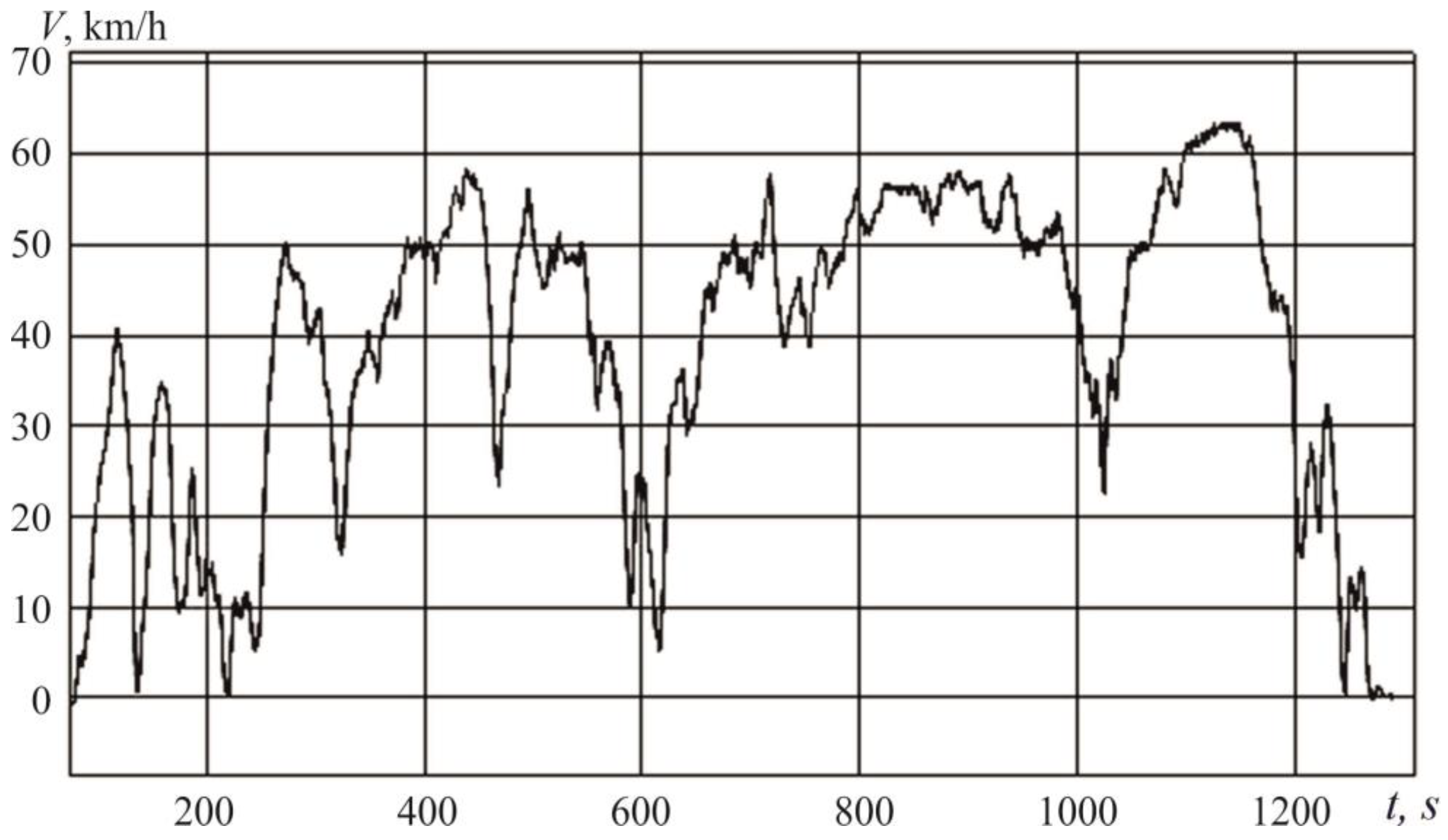
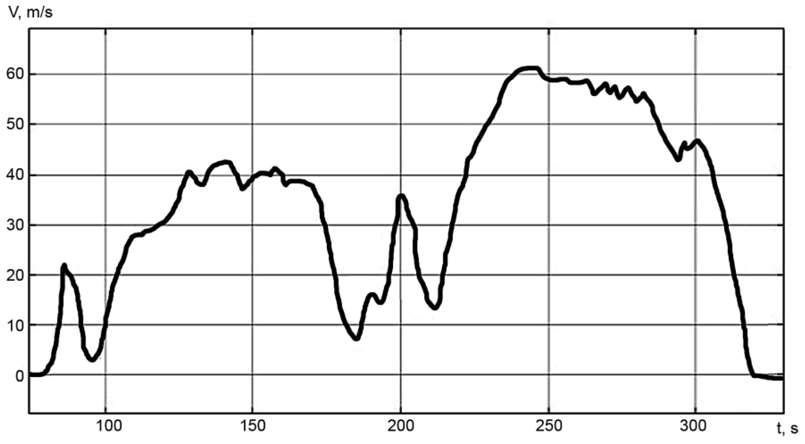
The first route was a mixed traffic cycle with low speed sections of urban traffic as well as motorway driving [24,25]. The electric vehicle was travelling empty and the mass was 10,000 kg. Figure 1 shows the dependence of speed on time along the route.
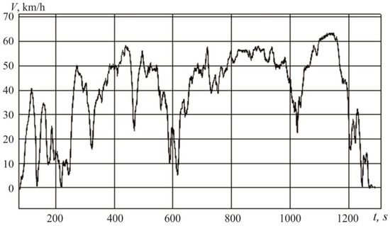
Figure 1.
Dependence of travelling speed on time of an electric car.
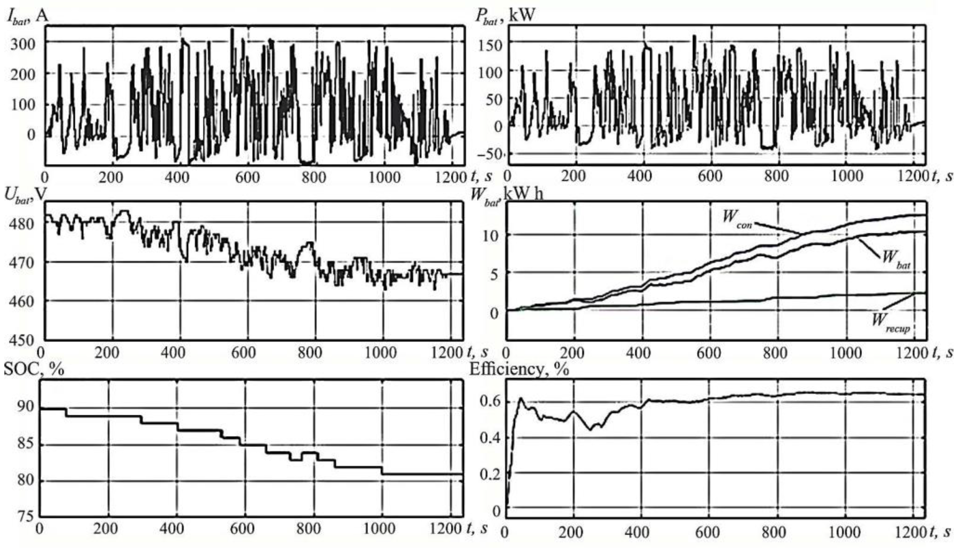
Figure 2 shows the characteristics of the traction electric driving system of the electric vehicle recorded while travelling along the route.
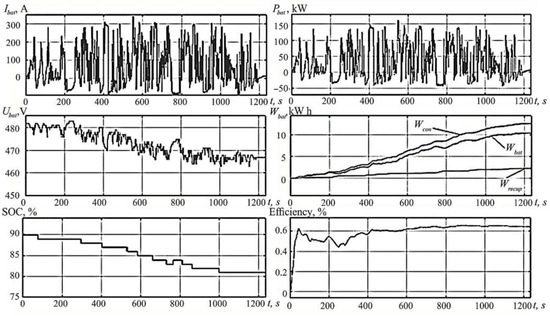
Figure 2.
Energy characteristics of the power plant of a heavy-duty electric vehicle.
From the graphs in Figure 2, it can be determined that the average battery current per cycle was 118 A (0.6 C). The degree of charge decreased from 90% to 82%.
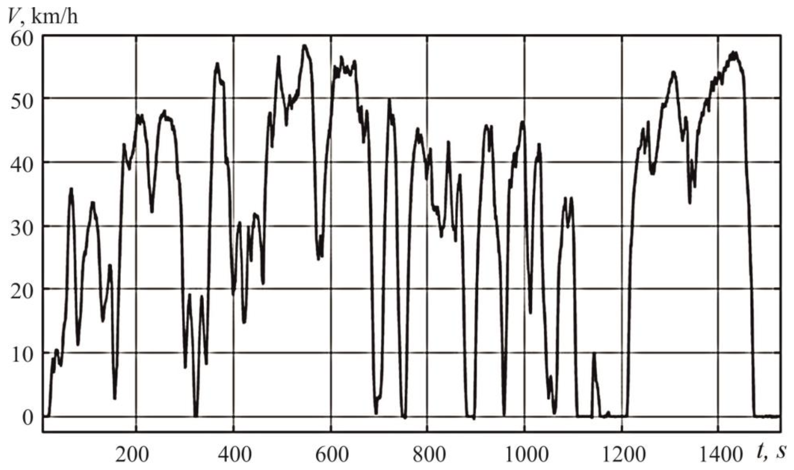
For the second route, in which the electric vehicle moved whilst loaded, the mass was 16,000 kg. Figure 3 shows a graph of the speed of the electric vehicle travelling along the route.
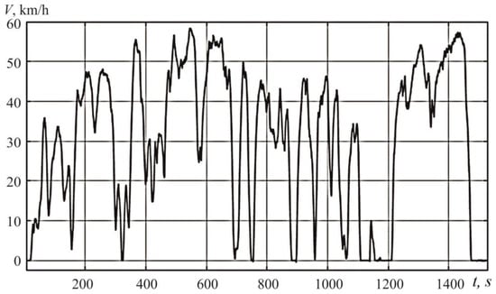
Figure 3.
Time dependence of speed along the route of a fully loaded electric vehicle.
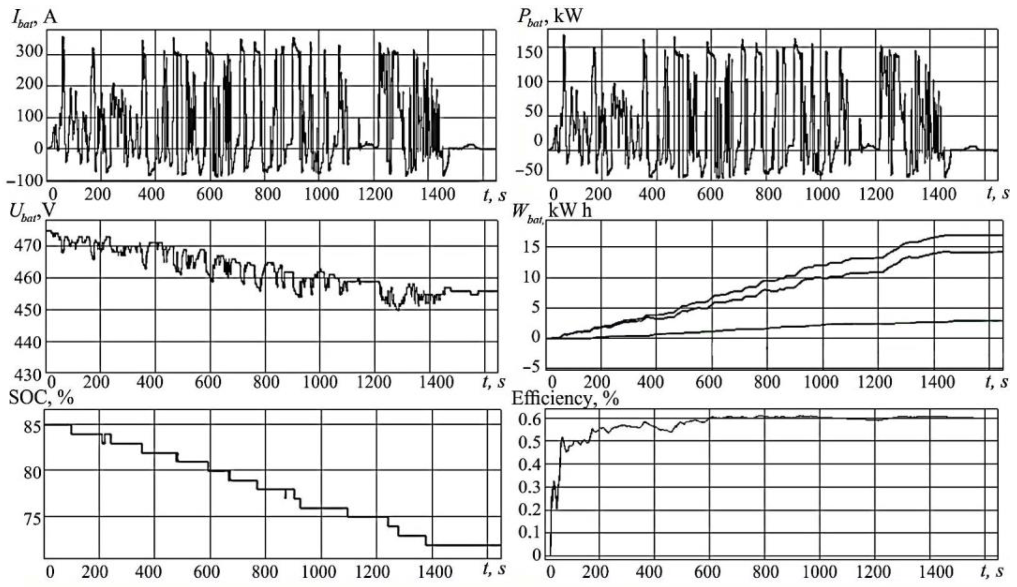
The average battery current per cycle was 140 A (0.7 C). The degree of charge decreased from 85% to 72%.
At the same time, the electric vehicle itself had equipment on board that captured the following characteristics:
- Ibat—the battery current;
- Pbat—the capacity of the battery;
- Ubat—the battery voltage;
- Efficiency—the coefficient of efficiency of the system;
- Wbat—the energy given up by the battery;
- SOC—the degree of charge.
These characteristics were obtained using CAN bus communication technology [26,27] and were recorded throughout the cycle (Figure 4).

Figure 4.
Energy performance of a fully loaded electric vehicle.
As a result of the tests, it was found that the electric vehicle was capable of travelling the two routes (Table 1) under consideration with a partial load (13,600 kg) and whilst fully loaded (16,000 kg). In this case, the depth of discharge can be seen in the SOC(t) plots in Figure 2 and Figure 4, respectively.

Table 1.
Test cycle parameters and test results of the electric vehicle.
To investigate the aging process of the battery [27,28], a system of equations describing the dependence on the battery temperature (), charge level () and values of charge and discharge currents () was compiled [27].
The United States Advanced Battery Consortium defines two operational modes for PHEVs: charge-depleting (CD) and charge-sustaining (CS). The ratio of CD-CS to the total operating time is then defined as the following ratio:
which indicates the fraction of time spent in CD mode over the total operation time. Therefore, corresponds to CD operation, i.e., all the operating time is spent in CD mode. corresponds to CS operation, i.e., all the operating time is spent in CS mode. Ratios such that correspond to mixed operation, i.e., the total operating time is divided between CD and CS modes.
- is the estimated loss of battery capacity during the experiment;
- is the minimum state of charge of a cell;
- is the minimum state of charge of a cell;
- is a factor depending on the degree of charge and the ratio of charge time to discharge time.
3.1. Mathematical Modelling of the Traction Electrical Equipment System of an Electric Truck
In order to determine the charging and discharging currents of the battery pack when driving a standardised cycle [29,30,31], a mathematical model of the traction electrical equipment system of an electric vehicle was developed in this work [32]. The mathematical model of an electric vehicle allows us to obtain the performance characteristics of the battery under different driving cycles [33].
The development of the mathematical model involved several steps:
- The development of a mathematical model that takes into account the mechanical characteristics of the vehicle (VT);
- The verification of the obtained data with the results of vehicle test runs, by comparing the acceleration characteristics in the simulation with the real characteristics when driving in an acceleration cycle on a straight road;
- The integration of the mechanical model with the electrical model in order to calculate the energy performance with reliable parameters of the traction electrical equipment system (TES) and dynamics of the vehicle.
The mathematical model contains a battery pack that can be configured for different parameters and chemical compositions [34,35]. This study presents a mathematical description of a squirrel cage induction machine [36]. This type of electric motor is used in the electric portal bridge of an electric vehicle [37,38].
The mathematical model is formed using specialised software. The main extension packages used in this study are Matlab Simulink (v9.7) and PowerSystemBlockset v2.2. The widely developed Simulink extension is most adapted for the analysis and synthesis of various systems [39,40]. This extension provides a variety of possibilities, ranging from structural (mathematical) representations of the system to the generation of codes in high-level languages and the subsequent programming of microprocessors, according to the structural diagram of the model [41].
The parameters of the Mitsubishi electric truck were selected for calculations of basic vehicle characteristics. The vehicle parameters are shown in Table 2.
Table 2.
Vehicle parameters and traffic conditions.
The characteristics required for the calculations can be determined according to the following expressions [42]:
The required traction force on the drive wheels, measured in N, is as follows:
where Ff is the rolling resistance force of the vehicle:
Fa—the acceleration/deceleration resistance—is as follows:
where δ is the rotating mass factor;
Fv—the aerodynamic drag—is as follows:
Fα is the force of resistance to uphill movement, shown as follows:
The required torque on the drive wheels is as follows:
The traction motor shaft speed (TM) is as follows:
The required torque on the TM shaft is as follows:
The drag torque on the TM shaft is
The required power on the TM shaft can be calculated by the following formula, kW:
The actual speed of the electric vehicle [43] is calculated according to the TM shaft speed using the following expression:
The Motor Vehicle Acceleration (MVA) is as follows:
Information about the value of the resistance torque on the TM shaft (Mc) serves as an input parameter for the mathematical model of the TM [44]. The data on the required values of torque, speed and power on the TM shaft are used in calculating the load moments on the TM [45,46].
The process of model creation starts with the mathematical description of the traction motor used as part of the electric portal bridge. The initial data are presented in Table 3.
Table 3.
Parameters of the electric motor installed in the electric portal bridge.
The determination of the energy performance of the system [47,48,49] was proposed to be carried out by means of a mathematical model of STEO.
A functional diagram of the generalised model of the electric vehicle’s traction electrical equipment system, made in the Matlab mathematical modelling environment, is shown in Figure 5.
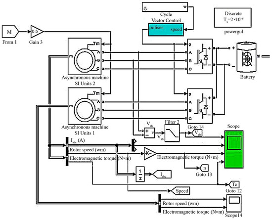
Figure 5.
Mathematical model of traction electrical equipment of an electric vehicle.
The mathematical model includes the following:
- An electric machine model (two asynchronous electric motors which are integrated in an electric portal bridge);
- A model of the electric energy conversion and control system of the traction electrical equipment (two inverters, for each electric motor);
- A model of the system of calculation of traction forces on the shaft of electric motors;
- An inverter control system model.
In addition, the scheme uses measuring devices and auxiliary blocks [50] to perform mathematical modelling and determine the characteristics of the system during given driving cycles.
3.2. Mathematical Modelling of an Electric Portal Bridge
In the ZF AWE 150 electric portal axle, each drive wheel is connected to a gearmotor [51,52,53]. An asynchronous motor with a squirrel cage rotor is used as the electric motor [54]. The speed control is performed by vector control. The issues of mathematically modelling AC electric drives have been dealt with by many scientists; the results of these studies are reflected in [55,56].
The mathematical modelling of the traction motor is based on the mathematical model of the induction motor (AM), which is represented in the substitution diagram shown in Figure 6.
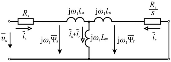
Figure 6.
Substitution diagram of asynchronous machine.
The vector equations of voltages [57] of AM windings can be graphically represented by an electrical diagram. Expressing the terms included in the vector equations——we obtain
where:
- are the stator and rotor flux-coupling vectors, respectively;
- —voltage vectors on the stator and rotor windings;
- —vectors of currents in the stator and rotor windings;
- Rs, Rr—active resistances of the stator and rotor windings;
- Ls, Lr—total inductances of the stator and rotor windings;
- Lm—mutual inductance of the stator and rotor windings (total inductance of stator winding from the main magnetic flux);
- —the angular velocity of the coordinate system;
- —the angular frequency of rotation of the rotor of an electric machine with one pair of poles.
Considering the expressions of the total inductances, Ls and Lr [58], Equation (13) will take the following form:
After grouping the summands, we obtain
In the stator and rotor voltage equations (Equation (15)), there is a common term, , which causes the presence of the magnetising branch in the circuit diagram—common for the stator and rotor circuit [59].
Expressions (15) are written in a coordinate system rotating with arbitrary velocity, ωk. As a special case from the AM equations in the synchronous coordinate system [60], occurring at ωk = ω1, we can obtain the stress equations for the static mode of AM.
Taking into account expressions (15) and considering that, in static mode in the synchronous coordinate system, , , and ω1 − ω = ω2 = σω1, we can write down the AM equations in a steady state (where s is the slip of the AM rotor):
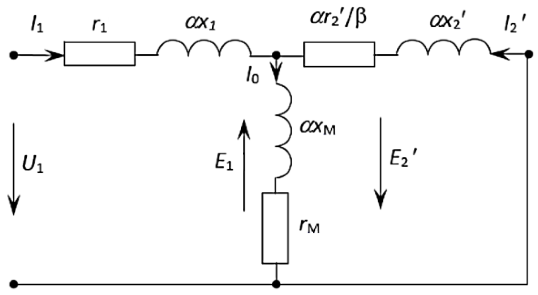
Taking the moduli of the vectors () equal in magnitude to the corresponding amplitudes of the phase voltage (U1) and currents (I1 and I2), the substitution scheme shown in Figure 7 will be valid for the induction motor [61,62].

Figure 7.
T-substitution diagram of an induction machine.
Figure 7 is labelled with the following:
r1, x1, xm, x2′, r2′—active and inductive resistances in the AM substitution diagram corresponding to the nominal mode.
and β are relative values of stator current frequencies (f1) and rotor current frequencies (f2), respectively:
f1n is the stator current frequency in nominal mode.
In the absence of external static torque on the shaft, the motor connected to the network will rotate at a speed close to synchronous [21,63,64]. In this case, the energy necessary to cover losses is consumed from the network. If the rotor rotates at a synchronous speed due to an external force, the network will cover only the losses in the stator, and the losses in the rotor (mechanical and steel) will be covered by the external force [65].
In the motor mode, when the rotating magnetic field crosses the stator and rotor winding conductors in the same direction, the stator EMF (E1) and rotor EMF (E2) coincide. At w = w0, EMF is not induced in the rotor; i.e., it is equal to 0. At w > w0, the stator winding conductors are crossed by the rotating field in the same direction, and the rotor conductors are crossed by the rotating field in the opposite direction.
The rotor EMF (E2) changes its sign to reverse; the machine enters the generator mode with energy recovery. As for the current, only its active component changes its direction. The reactive component at negative slip keeps its direction. This is also evident from the expression for the rotor current (at S < 0 and S2 > 0).
The same conclusions can be drawn from the analysis of active (electromagnetic) and reactive powers. Indeed, it follows from the expression for PЭM that at S < 0 PEM > 0.
i.e., the active power changes direction (is transferred to the battery), and from the expression for Q2, it follows that, at S < 0, the reactive power of the secondary circuit (Q2) keeps its sign regardless of the mode of operation of the machine.
This means that an induction machine in both motor and generator modes consumes the reactive power required to generate the magnetic field [66].
The following equations must be used to determine the slip and electrical angle of rotation (θ):
where wr is the field rotation frequency and wm is the mechanical rotor speed.
The rotor frequency is calculated using the following formula:
where ψ is the rotor flux.
Lm—the main (equivalent) inductance—characterises the part of the flux that is coupled to the stator and to the rotor and participates in torque generation. In the linear section of the motor magnetisation curve, the main inductance is a constant value. At saturation of the motor magnetic core, the value of the main inductance decreases [67].
where and are the inductances from the dissipation field from the currents of the other two windings.
Tr is the time constant of the rotor winding:
The electromagnetic torque of an induction machine can be found by the following formula:
where Zp is the number of pole pairs of the motor [68].
The equation of motion of the actuator will be written as
where Mc is the static load moment; w is the angular frequency of rotor rotation, rad/s; and J is the moment of inertia of the actuator reduced to the motor shaft.
Transition to Orthogonal Coordinate System
For the system of equations written with respect to the stator current and rotor flux coupling in coordinates (x,y), we make a transition to the orthogonal coordinate system (d,q) oriented along the rotor flux-coupling vector. In this case, wk = wψ, Ψrq = 0, and Ψrd = Ψr.
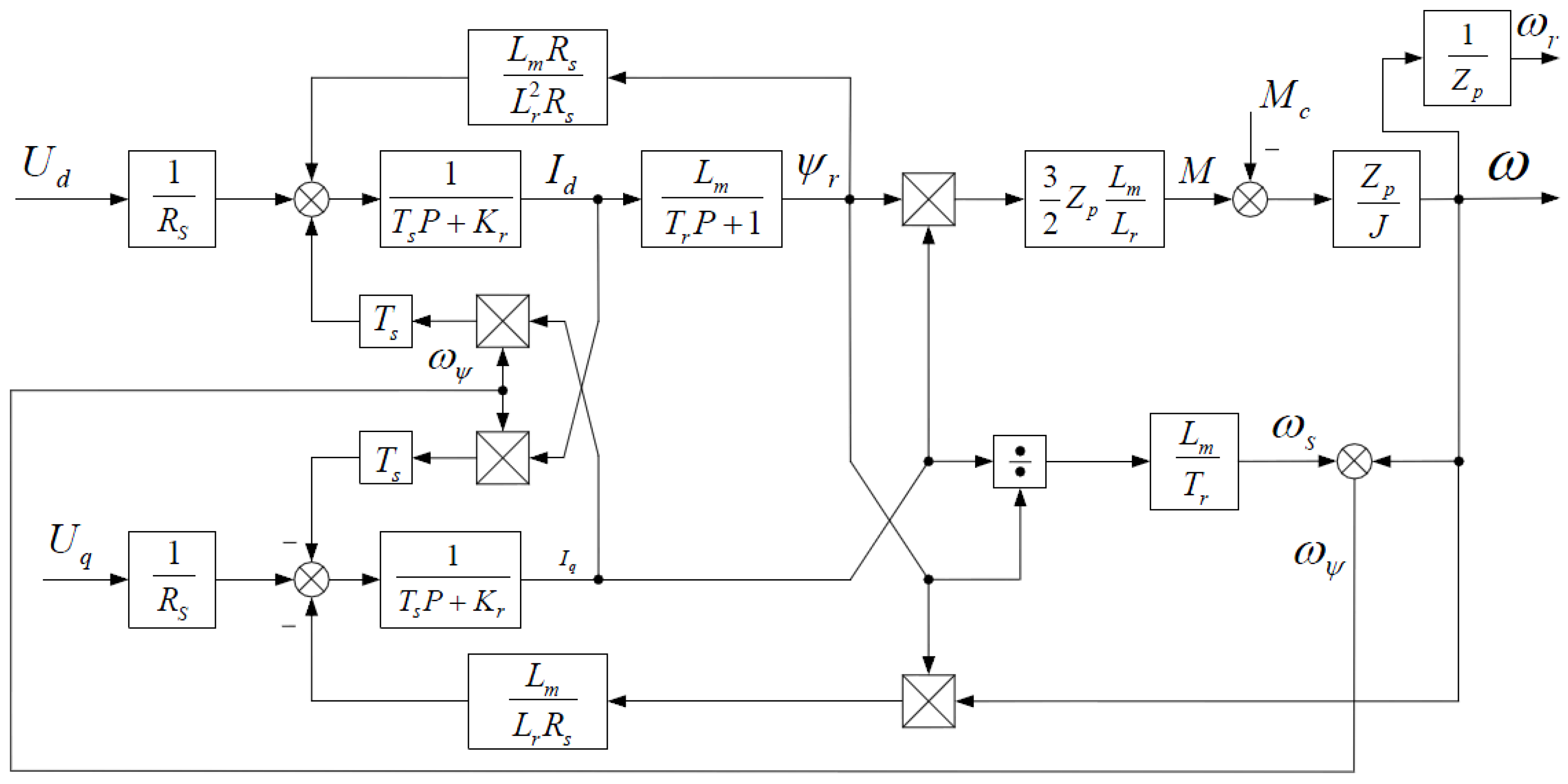
The mathematical model of the induction machine in the orthogonal coordinate system is synthesised and presented in Figure 8.
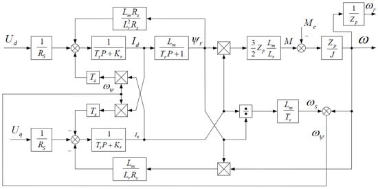
Figure 8.
Structural diagram of AM in coordinates (d,q).
In steady-state modes of motor operation, all transformed variables turn out to be constant values. In this connection, this system of equations is very convenient for calculations of processes in the machine and for the synthesis of the vector control system in coordinates (d,q).
The magnetising circuit saturation effect can vary by up to 30% in the operating modes of the drives. Current–current regulation to compensate for saturation is required in the following modes:
- (1)
- When the drive is operated at speeds higher than the rated speed (in the second speed control zone in constant power mode), field weakening occurs;
- (2)
- Optimisation of the power drive requires load-dependent magnetising flux control; one of the following methods is used to account for saturation effects: the static inductance method or the dynamic inductance method.
The method of static inductance is usually used for the synthesis of drive control systems, which gives sufficiently high accuracy in the description of dynamic processes. In this method, the nonlinearity of the magnetising circuit is specified tabularly or by means of analytical approximation.
The theoretical dependencies shown in this section form the basis for the construction of a vector control system for an electric vehicle with an induction motor, which is used when there are increased requirements for the dynamic or static characteristics of the control of the output variables of the drive, as well as in cases where the regulated variable is the torque.
A distinctive feature of using the described theory of electromechanical energy conversion in an alternating current electric machine is its integration into the system of a complex matmodel, where the entire range of characteristics and parameters that determine the energy performance and specificity of the traction current source operation is taken into account.
3.3. Mathematical Model Considering Mechanical Characteristics of the Vehicle and Subsequent Verification of Traction Characteristics
In order to observe the mechanical characteristics in an induction motor, it is necessary to carry out system modelling over the entire motor speed range.
The calculation of speed is carried out using Formula (6). In order to calculate the tractive force as torque on the motor shaft, the following formula must be used:
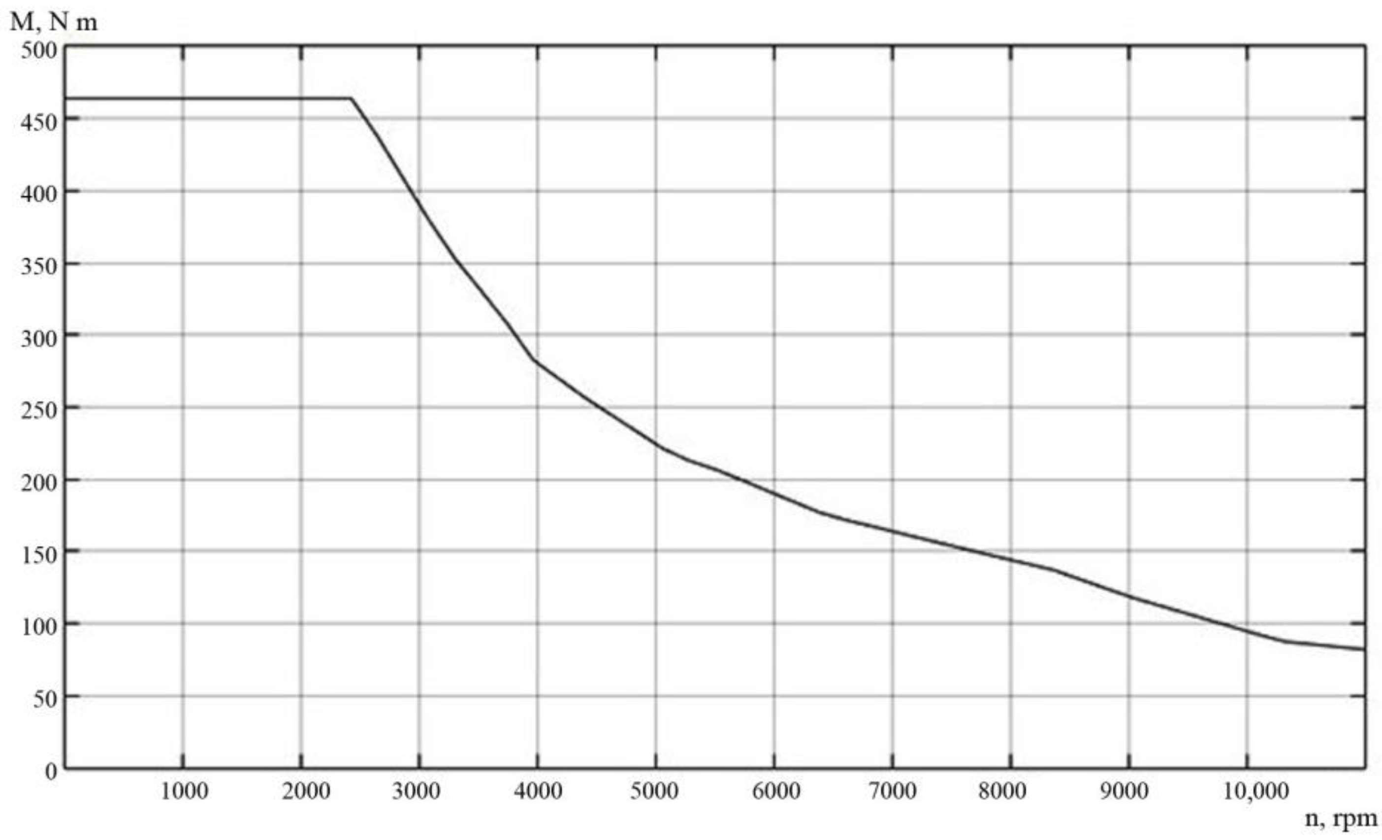
The mechanical characteristics for maximum power are calculated by the ratio of power to speed; the external characteristic of the motor is shown in Figure 9.

Figure 9.
External characteristic of the electric motor.
The maximum traction motor speed is 11,000 rpm. The maximum torque is 450 Nm. These characteristics allow for the creation of a verification mechanical model of the electric vehicle (Figure 10). The model allows us to clarify the traction–dynamic characteristics of the electric vehicle by comparing the acceleration characteristic in the simulation with the real data obtained in experimental studies.

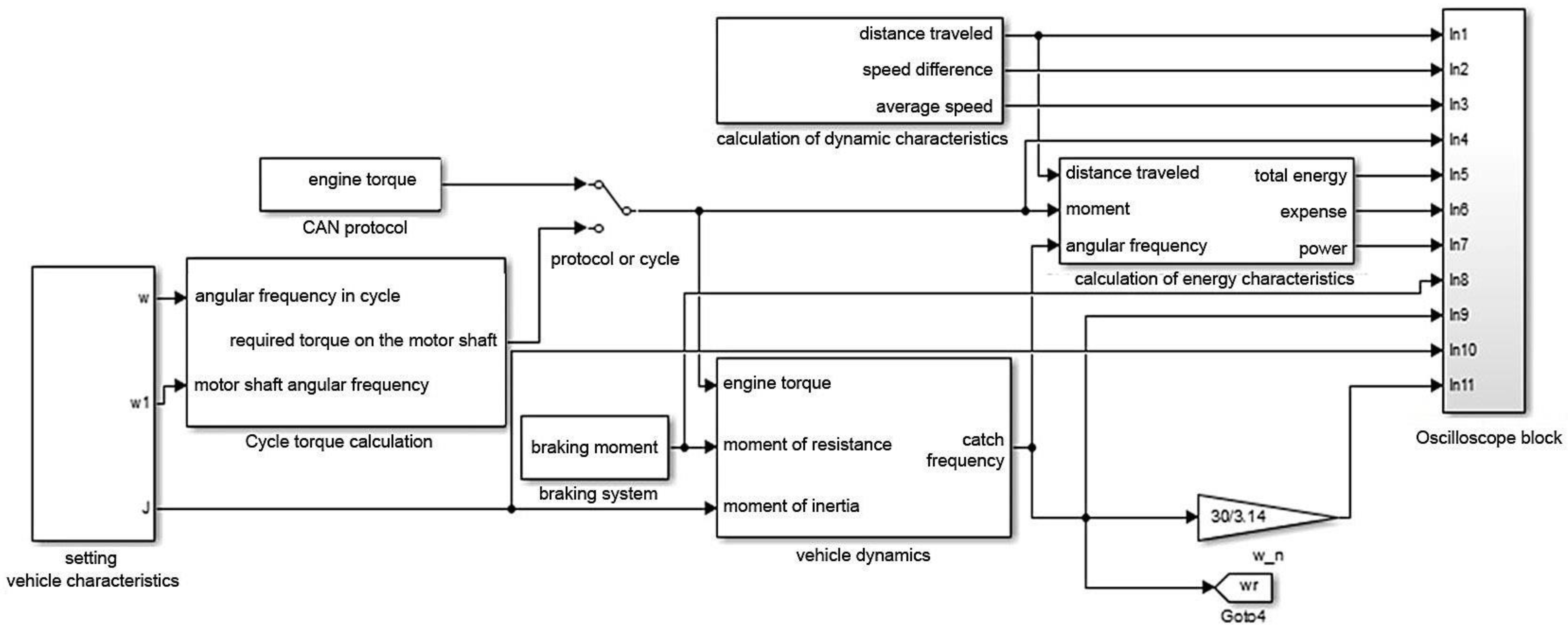
Figure 10.
Structural diagram of the mechanical model of an electric vehicle.
The model consists of the following blocks:
- A vehicle characterisation unit;
- A block for calculating the torque by cycle;
- A vehicle dynamics calculation unit;
- A braking system unit;
- A dynamic characteristic calculation unit
- A block for calculating energy characteristics;
- An oscilloscope unit.
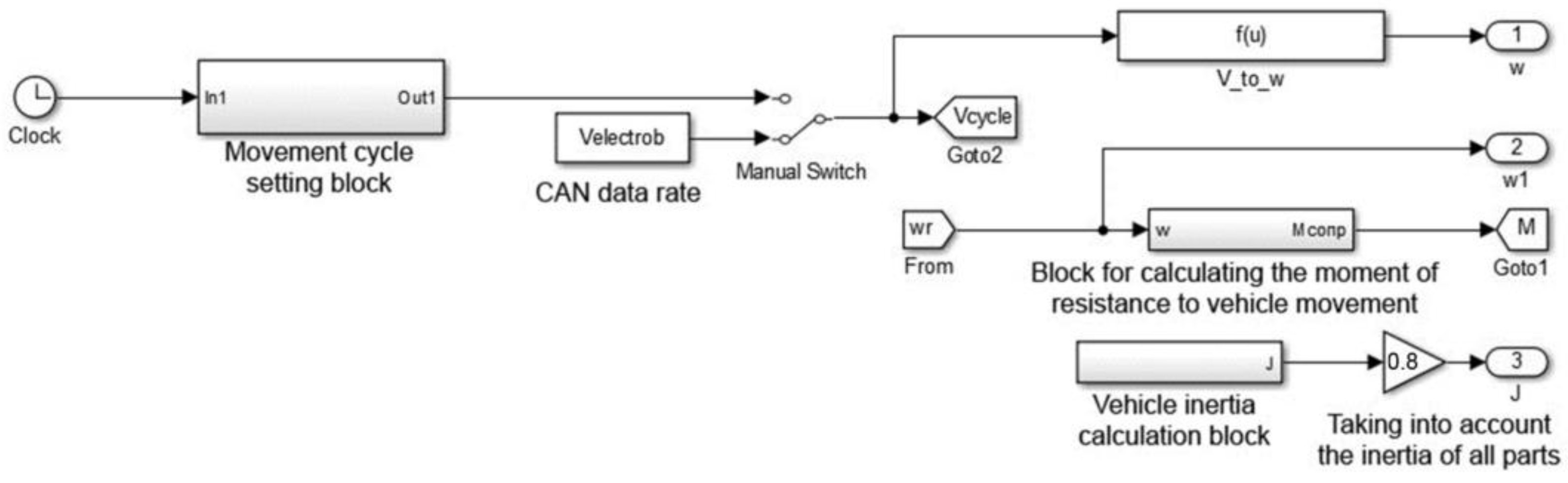
The vehicle characterisation block (Figure 11) consists of the following sub-blocks:
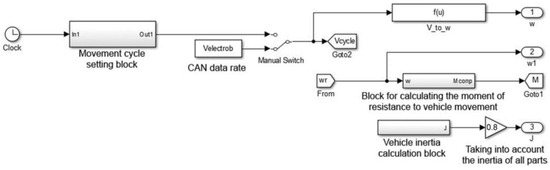
Figure 11.
Vehicle characterisation block.
- A motion cycle setting unit;
- A unit for calculating the moment of resistance to vehicle movement;
- A vehicle inertia calculation unit.
The motion cycle setting block is shown in Figure 12; it consists of tables with data, in which motion cycles are described in the form of speed vs. time dependencies. The blocks are numbered and connected to a multiport switch. The switch allows you to quickly change the motion cycle when setting the initial data during the modelling process.

Figure 12.
Motion cycle setting block.
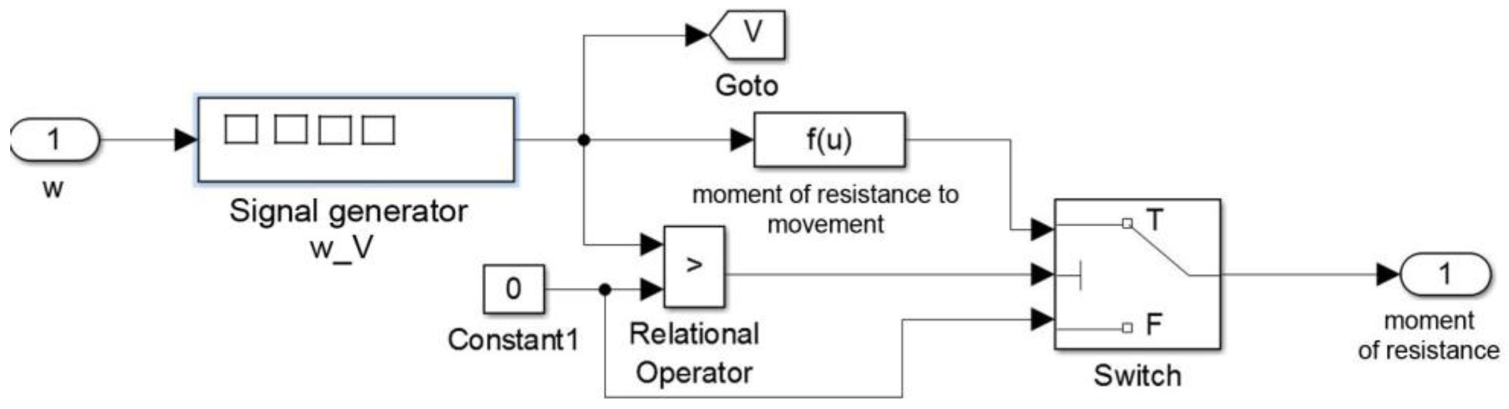
The block converts the value of the angular frequency of the engine shaft rotation into the linear speed of the car using the function “w_V”, which is calculated according to formula (11). After converting the frequency into speed, the signal is fed to the block “Moment of resistance to motion” (Figure 13), which realises the dependence (8). The blocks “Constant1”, “Relational Operator” and “Switch” (hereinafter, the original names of the blocks used in Simulink software are given) are necessary for the programme zeroisation of resistance forces when stopping the vehicle. This function is designed to eliminate possible errors in calculation and the incorrect determination of drag forces at the moment when the vehicle comes to a complete stop.
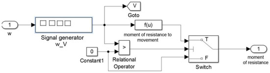
Figure 13.
Block for calculating the moment of resistance to vehicle movement.
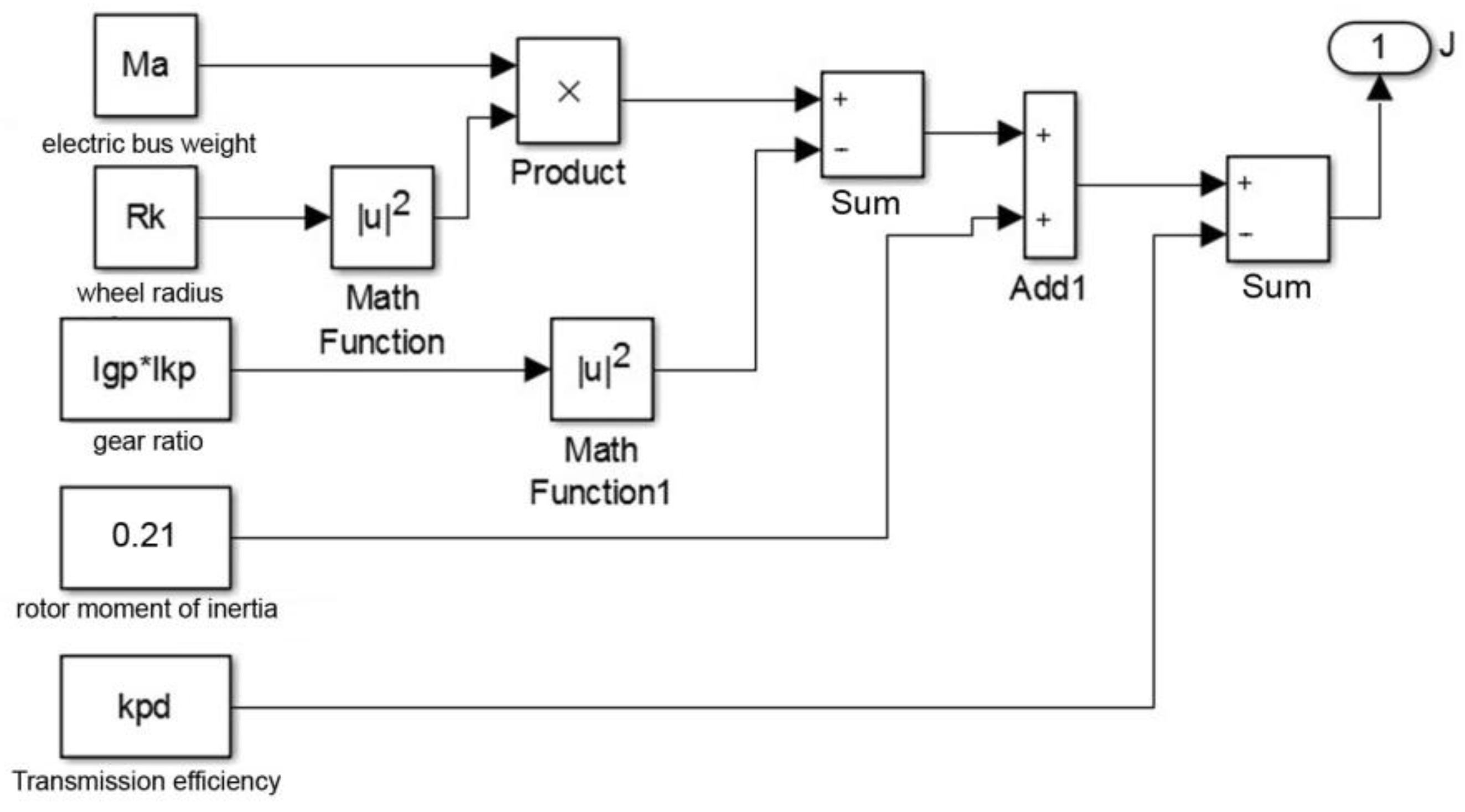
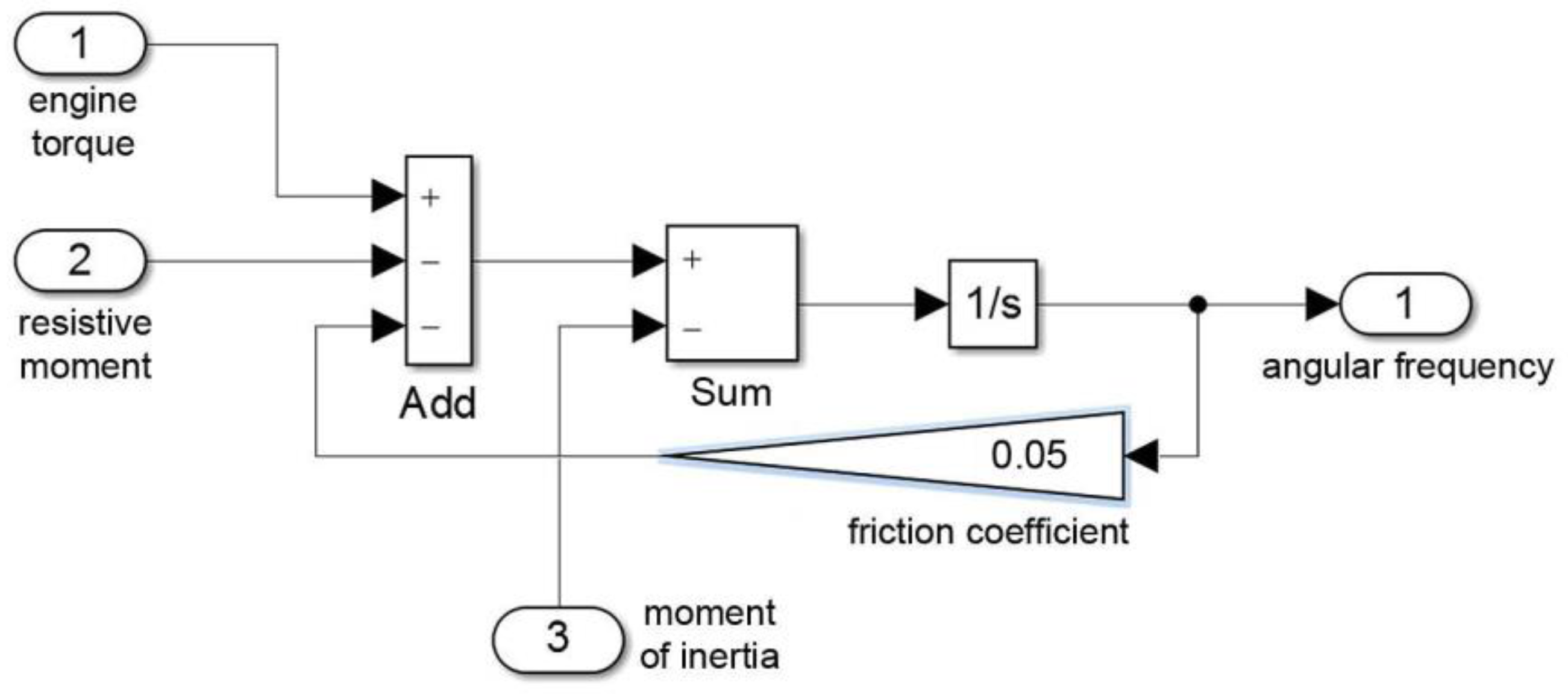
The block in Figure 14 calculates the vehicle’s moment of inertia using the following formula:
where Ft is the coefficient of viscous friction for motor shafts and Ft is 0.03 Nms.
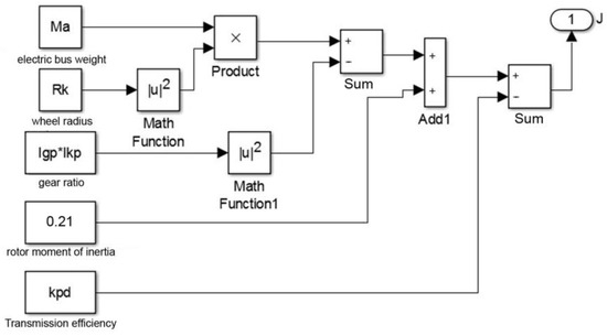
Figure 14.
Unit for calculating the moment of inertia applied to the motor shaft.
This formula allows you to find the approximate moment of inertia of the car. In order to find the real moment of inertia, it is necessary to verify the model.
The integration of the obtained acceleration value over time using the integrator block allows us to determine the angular velocity of the motor shaft. The blocks for calculating the dynamic and energy characteristics reflect the mathematical dependencies for the calculation of the travelled distance, the average speed in the cycle, useful energy, specific consumption and useful power on the shaft. The oscilloscope block contains oscilloscopes of all measured quantities.
In addition to receiving a signal from the motion cycle, the model facilitates the use of external speed information to compare the speed during mathematical modelling with the data registered via the CAN protocol. In this case, the data obtained as a result of calculations are fed to the block that calculates the error of the obtained results, and can also be sent to the oscilloscope block. To obtain data from the CAN protocol, the From Workspace block is used.
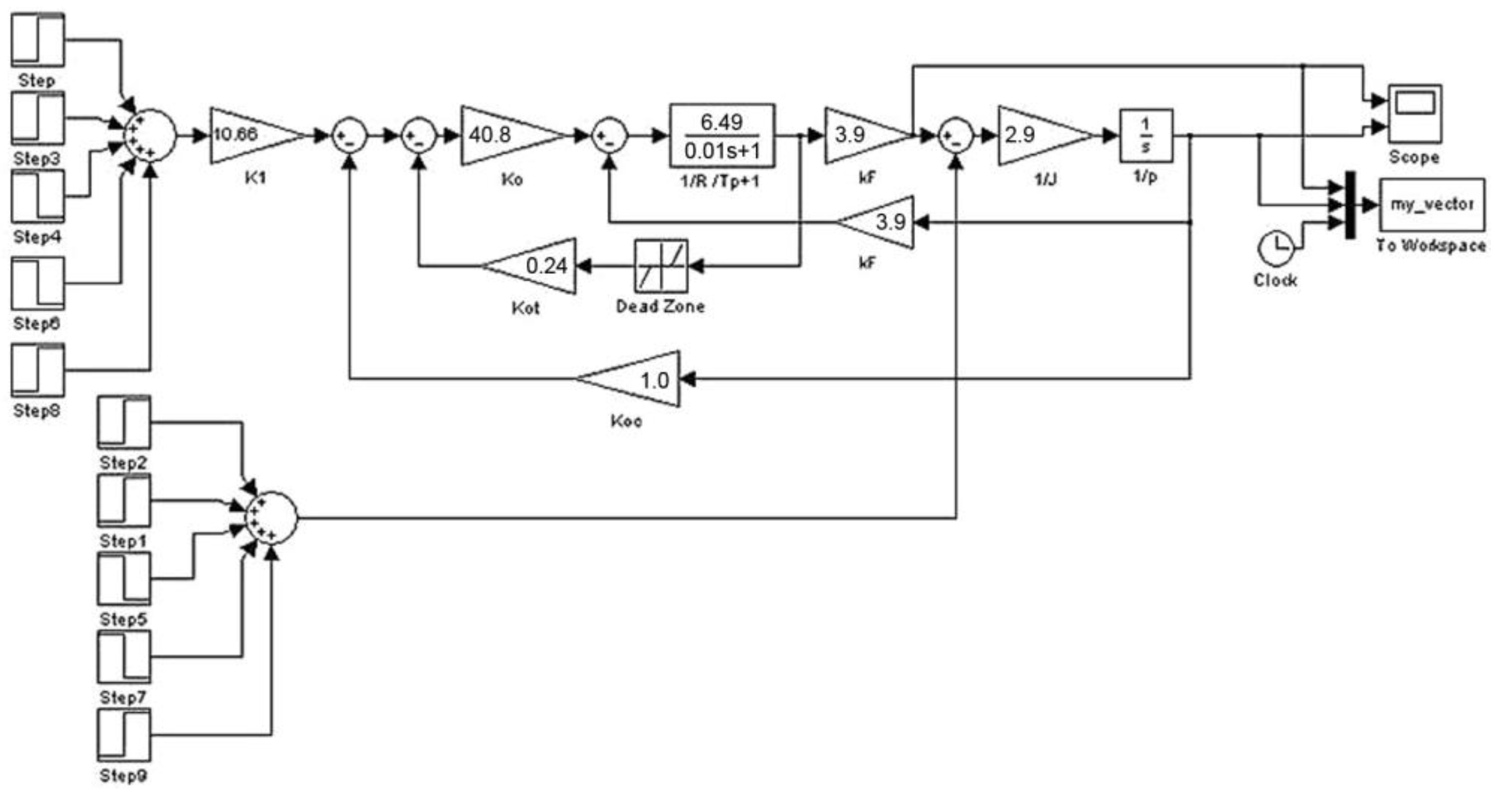
The structure of the block for calculating the required torque per cycle is shown in Figure 15.
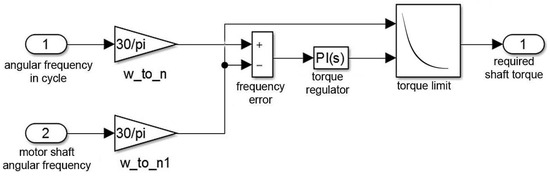
Figure 15.
Block for calculating torque by cycle.
The unit consists of a “PI controller” [69], which compares the error between the theoretical cycle-defined angular speed of the TM shaft and the actual speed. The output of the “PI controller” calculates the motor torque signal, including all losses [70]. The content of the torque calculation block is shown in Figure 16. Also, like the cycle assignment block, the submodel consists of data tables and a switch between characteristics. The submodel allows us to calculate the dynamic characteristics of the vehicle at all possible modes of operation of the electric vehicle.
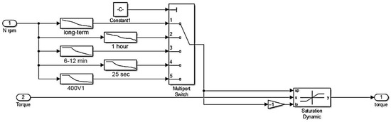
Figure 16.
Block for calculating the required torque in a driving cycle, taking into account the motor operating mode.
The model is equipped with a special unit designed to realise the OEM braking system. The OEM braking scheme is shown in Figure 17.
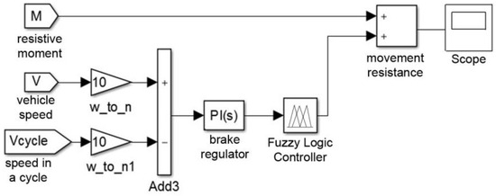
Figure 17.
Standard braking system.
The braking control system increases the drag torque on the motor shaft if the vehicle speed is higher than the speed in a given driving cycle [71]. The model is necessary when comparing the results from the test protocol. The electric vehicle uses regenerative braking in addition to the conventional braking system. The energy generated by the braking torque of the electric motor is used to charge the battery. However, when the battery is fully charged and cannot accept the energy, the regenerative torque must be limited, using the OEM braking system. The ratio of the mechanical braking system to the electrical braking system determines the efficiency and electrical energy consumption. When driving in a cycle, the braking system unit can be deactivated so that full energy recovery takes place. The “Saturation 1” block limits values above zero so that the controller only switches on the standard system when there is insufficient regenerative torque (Figure 18). The mechanical braking torque calculation block detects the error between the theoretical speed in the cycle and the actual speed, and uses the controller to add braking torque. When the regenerative torque is sufficient, the error between the speeds in braking mode is zero.
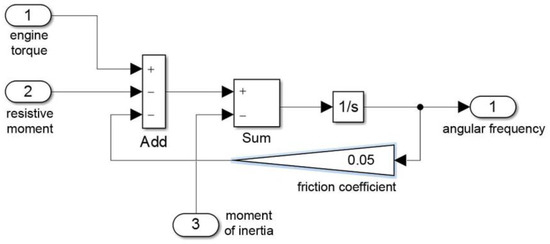
Figure 18.
Vehicle dynamics calculation block.
The integration of the obtained acceleration value over time using the integrator block allows us to determine the angular velocity of the motor shaft. The blocks for calculating the dynamic and energy characteristics reflect the mathematical dependencies for the calculation of the travelled distance, the average speed in the cycle, useful energy, specific consumption and useful power on the shaft. The oscilloscope block contains oscilloscopes of all measured quantities.
3.4. Mathematical Model of Vector Control of Asynchronous Electric Motor
This subsection considers the transition to the pulse-width method of output voltage generation, as well as the method of relay-vector formation of inverter control algorithms, in order to realise vector control of a traction electric drive. This method of control is used when there are high requirements for the dynamic or static characteristics for controlling the output variables of the drive, as well as in cases when the controlled variable is the torque on the shaft. The operating modes of an electric vehicle imply significant changes in the mechanical characteristics of the electric motor in a wide range, and regenerative braking is required, which requires the formation of motor control algorithms in the generator mode.
Transition to the pulse-width method of output voltage generation allows us to realise the following properties of the voltage converter (VC):
- The output current shape is substantially closer to sinusoidal, improving the rotation uniformity and extending the speed control range (the limitations on the speed control range from the voltage generation method are very small);
- A significant increase in the speed of the electric drive, since the power filter is actually excluded from the IF output voltage regulation channels;
- A significant improvement in the power factor of the IF as an energy consumer.
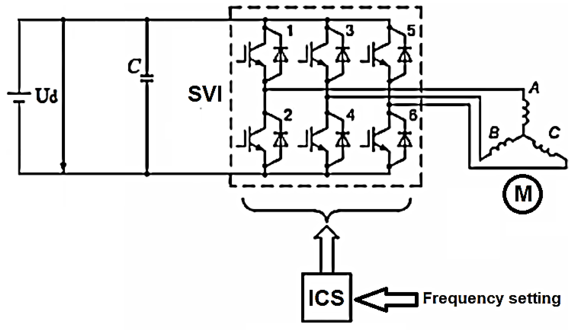
A frequency converter operating on the stator winding of an induction motor is shown in Figure 19.
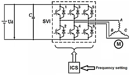
Figure 19.
Structure of voltage converter with DC source and controlled rectifier.
This includes a stand-alone voltage inverter (SVI) with an inverter control system (ICS) and battery (ICB). The power circuit of the inverter consists of six controllable switches, labelled in the figure with numbers 1–6.
These keys have double-sided conductivity. The keys are made on transistors providing current flow in the direct direction from the battery to the traction motor. Reverse conductivity is provided by reverse-current diodes included in parallel to the transistors. They create a circuit for reverse current flow during the switching of the transistors and in the braking mode of the motor.
Frequency control (w0эл) at the output of the inverter is carried out by influencing the inverter control system, in which the frequency reference signal is converted into the duration of the control signals applied to the inverter transistors in accordance with the established algorithm. The value of AC voltage amplitude at the inverter output is determined by the value of the rectifier voltage (Ud), from which the inverter output voltage is formed.
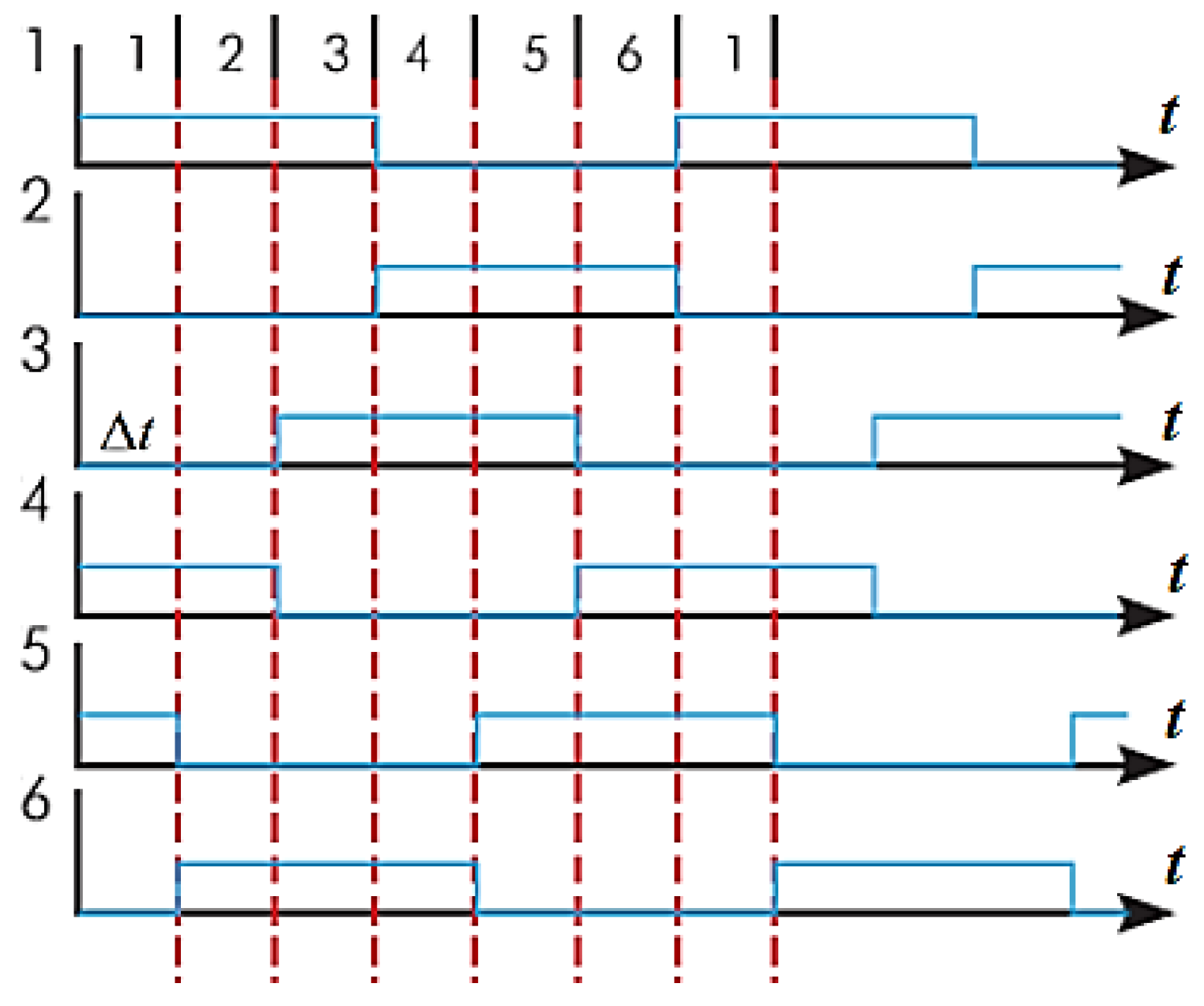
The state diagram of the inverter keys when the angular duration of the closed state of the keys (the open state of the transistors operating in the key mode) is equal to π is shown in Figure 20.
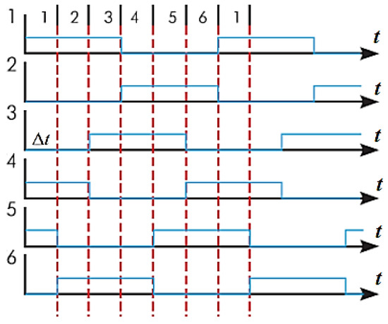
Figure 20.
Inverter key state diagram.
At any given moment of time, three keys are closed. The state of the keys changes every sixth part of the period, the duration of which in time units () is determined by the set frequency value at the inverter output, as follows:
Changing the frequency signal at the input of the inverter control system leads to a change in this duration, i.e., a change in the frequency (w0el) of the output voltage. The closing sequence of keys 1-2-3-4-5-6 in Figure 20 corresponds to a certain direction of motor rotation. To change it, this sequence must be reversed. The diagram shows that there are six key states, in which two even and one odd keys or one even and two odd keys are always closed. In addition to these, there are two zero states, in which keys 1-3-5 or 2-4-6 are closed and all three phases of the stator are closed to the positive or negative contact of the battery, which corresponds to zero voltage on the load. The inverter has the function of regulating not only the frequency, but also the amplitude of the main harmonic of the output voltage.
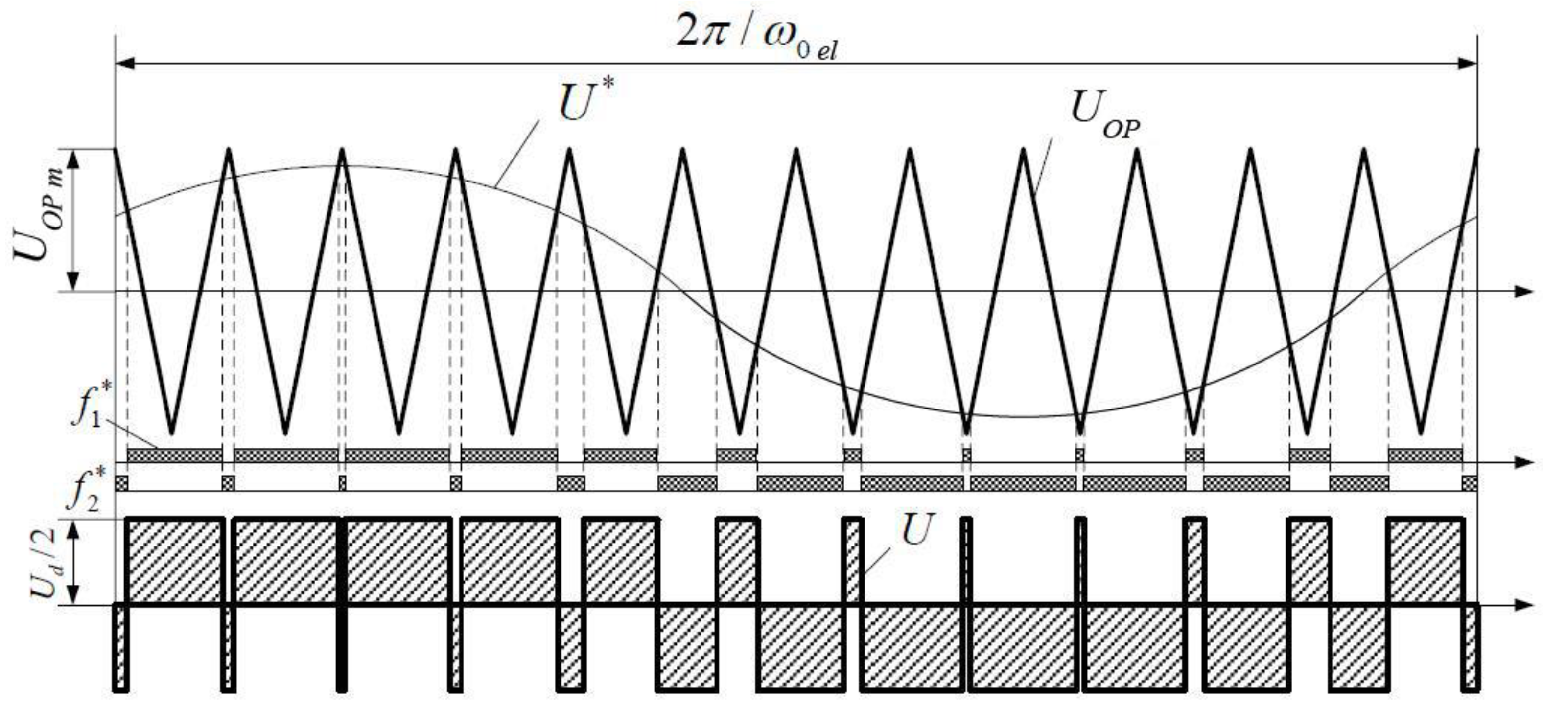
The principle of PWM generation is shown in the example of processes occurring in one phase of the inverter. The following notations are adopted in Figure 21:
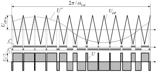
Figure 21.
Pulse width modulation principle on the example of a single-phase inverter.
- -
- U* is the inverter control signal;
- -
- UOP is the reference voltage;
- -
- f1* and f2* are the control signals of the upper and lower key of the inverter phase.
If the amplitude of U* does not exceed the value of UOP, the first harmonic of the voltage at the inverter output repeats the control signal in a certain scale. A change in its frequency results in a change in the frequency at the inverter output. A change in the amplitude of the control signal at a constant frequency will lead to a change in the ratio of the duration of positive and negative voltage pulses at the output, i.e., a change in the amplitude of its first harmonic. At high PWM frequencies and an active–inductive load, such as the stator winding, the load current is almost sinusoidal.
In Matlab, the Simpowersystems library provides an inverter block with variable parameters and configuration. For traction electric drive in the block, it is necessary to set the following parameters: the resistance of the snubbers (Rs) = 500 ohms; the capacitance of the snubbers (Cs) is set as “inf”, which means an infinitely large value and is equal to the absence of capacitive snubbers in the scheme.
In the field “Power Electronic device”, the parameter “IGBT/Diodes” is selected, which means the use of IGBT transistors with reverse-current diodes. Parameter Ron = 0.001; the internal resistance of the transistors is set by default.
The “Forward voltages” parameter is set to 1.4 V, which is the transistor trigger voltage.
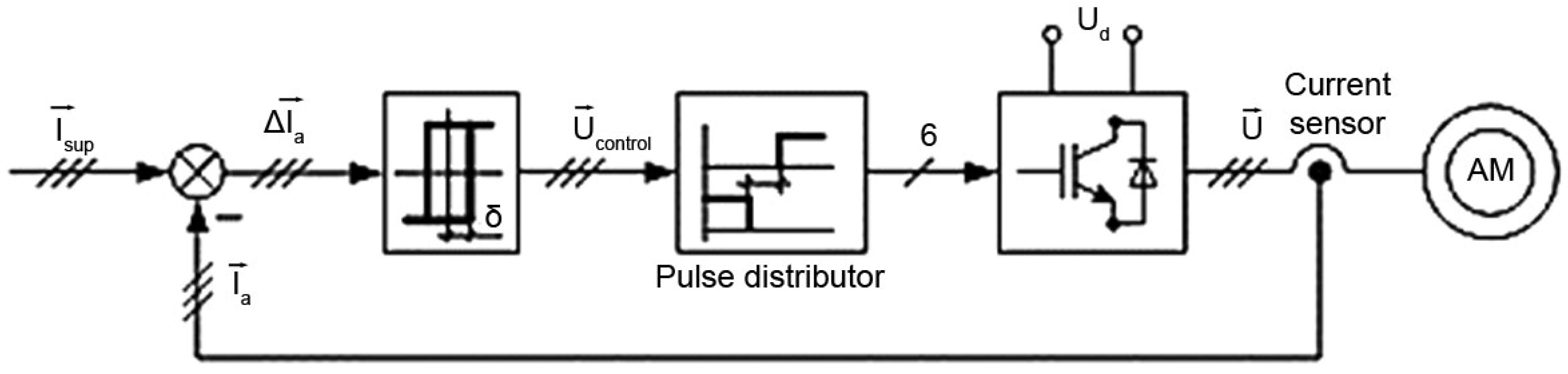
Regarding closed stator current loops, the application of the principles of relay-vector formation in voltage inverter control algorithms in a closed loop for tracking the instantaneous values of stator current errors allows us to significantly increase the speed of the control system and reduce the sensitivity of regulators (without forced modulation). A structural diagram of one of the simplest variants of the realisation of these principles is presented in Figure 22.

Figure 22.
Structural diagram of the current relay circuit.
The current control of the standalone inverter is a control method using current feedback. By coordinate transformation, the controller generates sinusoidal currents of a desired amplitude and frequency, which are compared with the actual stator currents. When the current exceeds the upper switch-on threshold, the lower switch of the inverter arm is switched off, while the upper switch, on the contrary, is switched on, causing the current to return to the threshold limit. In this way, the value of the current is monitored and controlled within the set limits. The amplitude and frequency of ripples is determined by the R,L parameters of the load and the width of the hysteresis loop of the relay element.
The components of the discrete control vector are formed according to the following equations:
where is the hysteresis of the relay current regulator; is the vector discrete function of current errors; and are components of the vectors of the set and real stator currents ( and respectively).
The pulse distributor (PD) distributes control signals to six inverter keys, taking into account the formation of delays in switching the keys of one phase. A realisation of the current relay circuit for three phases is shown in Figure 23.
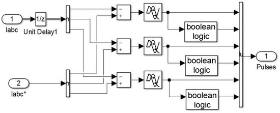
Figure 23.
Realisation of current relay circuit in Matlab Simulink environment (*—indicates inverter parameters).
The input signals of the model are not real, but they set the values of the stator current vector components in the coordinate system (d,q). This assumes that, in all operating modes of the drive, the stator current vector corresponds to its set value with accuracy to a small value determined by the hysteresis of the relay controller. In other words, in all operating modes of the drive (including dynamic modes), the conditions for the existence of a sliding mode in the relay current loop must be fulfilled:
where Ls and Rs are the inductance and active resistance of the stator phase;
is the scattering coefficient; and j = a,b,c.
Formula (37) shows that the conditions for the existence of the sliding mode impose restrictions not only on the real motor variables (stator current, the rate of change of the rotor flux circuit), but also on the derivative of the reference current. This can be ensured by sequential inclusion in the channels of Idz and Iqz, forming additional elements and realising algorithms with a nonlinear limitation to their rate of change. However, the electric drive turns out to be operable even without these additions, since the intervals of the current loop dropping out of the sliding mode at a step change in the set point are short-term (fractions of milliseconds), and the state observer has the properties of a low-pass filter.
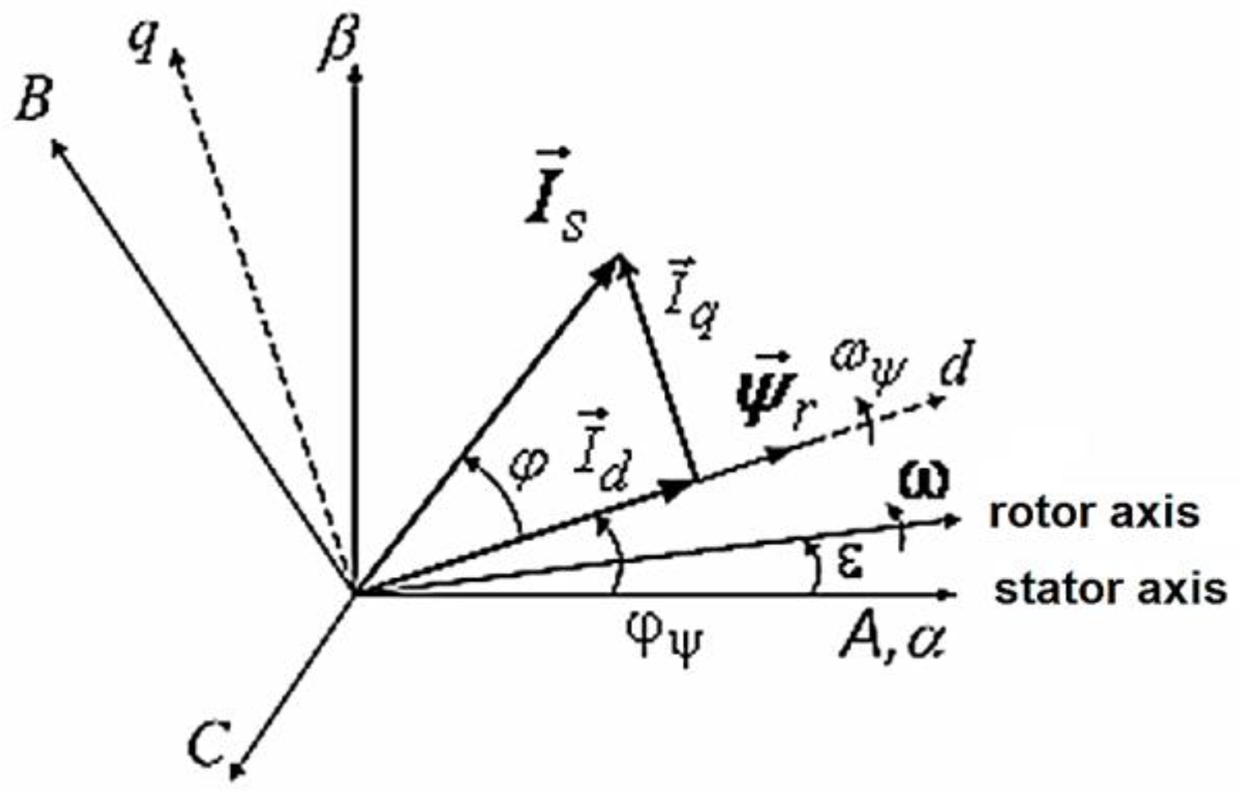
The fundamental principle of vector control is the orientation of the vector variables of the drive relative to each other. Orientation can be performed on almost any vector variable; however, it is common to select the variables whose orientation facilitates the simplest control system structure and the best dynamic and static properties of the drive.
The most widespread in vector control systems is the method of orienting variables to the rotor flux vector (Figure 24). This method is often called field orientation.
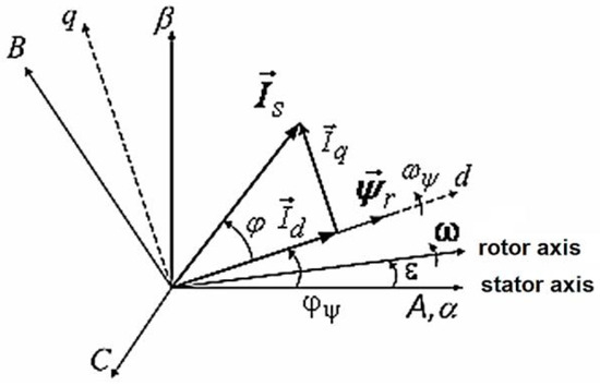
Figure 24.
Scheme of orientation of variables to rotor flux vector.
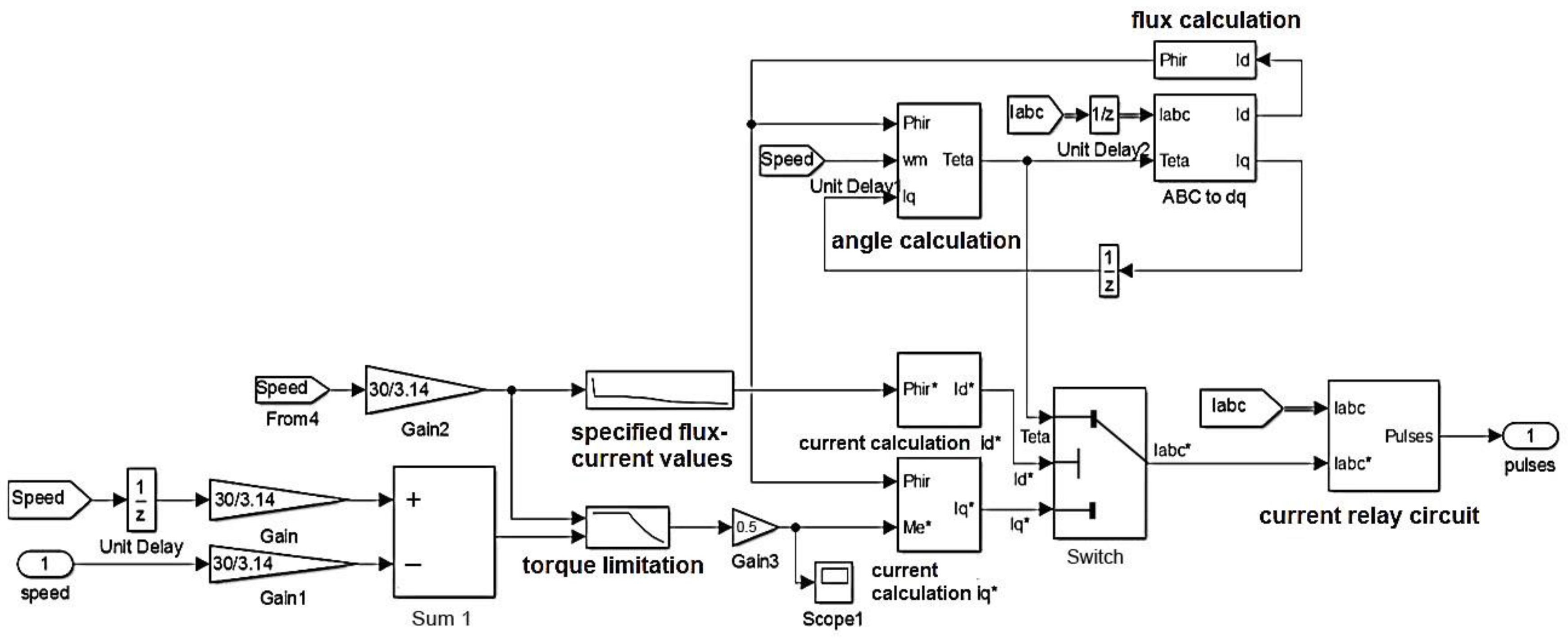
The specified provisions and mathematical dependencies are realised programmatically using Simulink. The component of the complex model of the vector control system is the structural diagram shown in Figure 25.
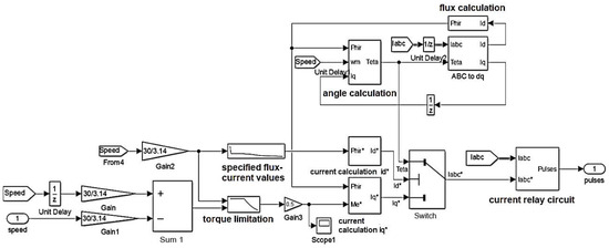
Figure 25.
Induction motor control system (*—indicates inverter parameters).
The shown structure of the control system is formed using dependences (38)–(43). The method of mathematical model formation using the specialised Simulink software for calculation studies of drive energy characteristics has an advantage over methods of direct solutions of equations describing the operation of simulated devices. Furthermore, it gives an opportunity to optimise and reduce the labour intensity of design studies, to obtain the most accurate results and to increase the calculation step. To determine the function of the rotor flux coupling change from the rotational speed, it is necessary to carry out mathematical modelling of the induction motor operation mode based on the external speed characteristic. The obtained dependence is shown in Figure 26. A sharp decrease in the value of flux coupling at low speeds is associated with large inrush currents, which must be reduced as the motor speed increases.
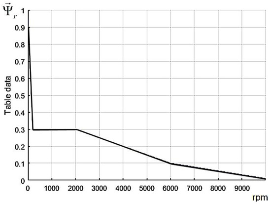
Figure 26.
Dependence of the asynchronous engine flux linkage on the rotation speed.
The ZF AWE 150 electric portal bridge, considered in this study, is a system that includes two traction electric drives. To calculate the energy characteristics in the model, two inverters and two asynchronous electric motors must be used. The electric motors are connected to the inverters. Thus, signals for the control of two independent AINs are synchronised, providing symmetrical control over traction motors. For the purposes of this study, the peculiarities of controlling the TEDs when turning the vehicle were not taken into account when modelling the vehicle motion.
For preliminary model adjustment in the first stage of computational studies, the following actions were performed:
- (1)
- For the optimal operation of the motor control system, it is necessary to set the minimum calculation step “Sample time”. To do this, the following commands are specified in the Matlab command line: T = 2.5000 × 10⁻⁶ >> Ts = T.
These commands set the discreteness (step) of calculation as 0.0000025 s, which allows us to realise high-frequency algorithms of traction drive control and to carry out fast reactions within the system to changes in traction modes.
- (2)
- Filling in the vehicle parameter menu in the “Cycle” block, the vehicle parameters are filled in according to the specification and the driving cycles are set in the dialogue box.
In the battery pack, the values of the nominal voltage, capacity, degree of charge and battery type are set.
After selecting the motor in the subsystem “Vector Control” in the blocks “flux calculation”, “angle calculation”, “current calculation Id*” and “current calculation Iq*”, it is necessary to enter the parameters of the TM: Rs, Lm and Lrμ.
4. Verification of the Mechanical Model with Real Test Results
To verify the vehicle dynamics in this study, the data obtained over the CAN bus during the testing of an electric vehicle in accordance with EN 1986-1:1997, “Electrically propelled road vehicles—Measurement of energy performances” [63], was used.
The following characteristics were measured as a result of the tests:
- The torques of the electric motors;
- The motor shaft speed;
- The actual speed of the electric vehicle.
The use of experimental data on driving in other conditions does not allow us to estimate the real drag forces acting on the wheels of the electric vehicle, because the drag moment reduced to the motor shaft will be greater on ascent and lesser on descent due to the presence of the drag moment when the vehicle is travelling on an uneven road [21,64].
Figure 27 shows the speed characteristics of the electric vehicle when driving on a standardised cycle.
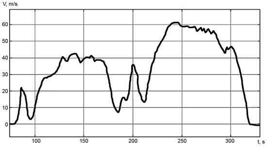
Figure 27.
Electric vehicle driving on a flat road.
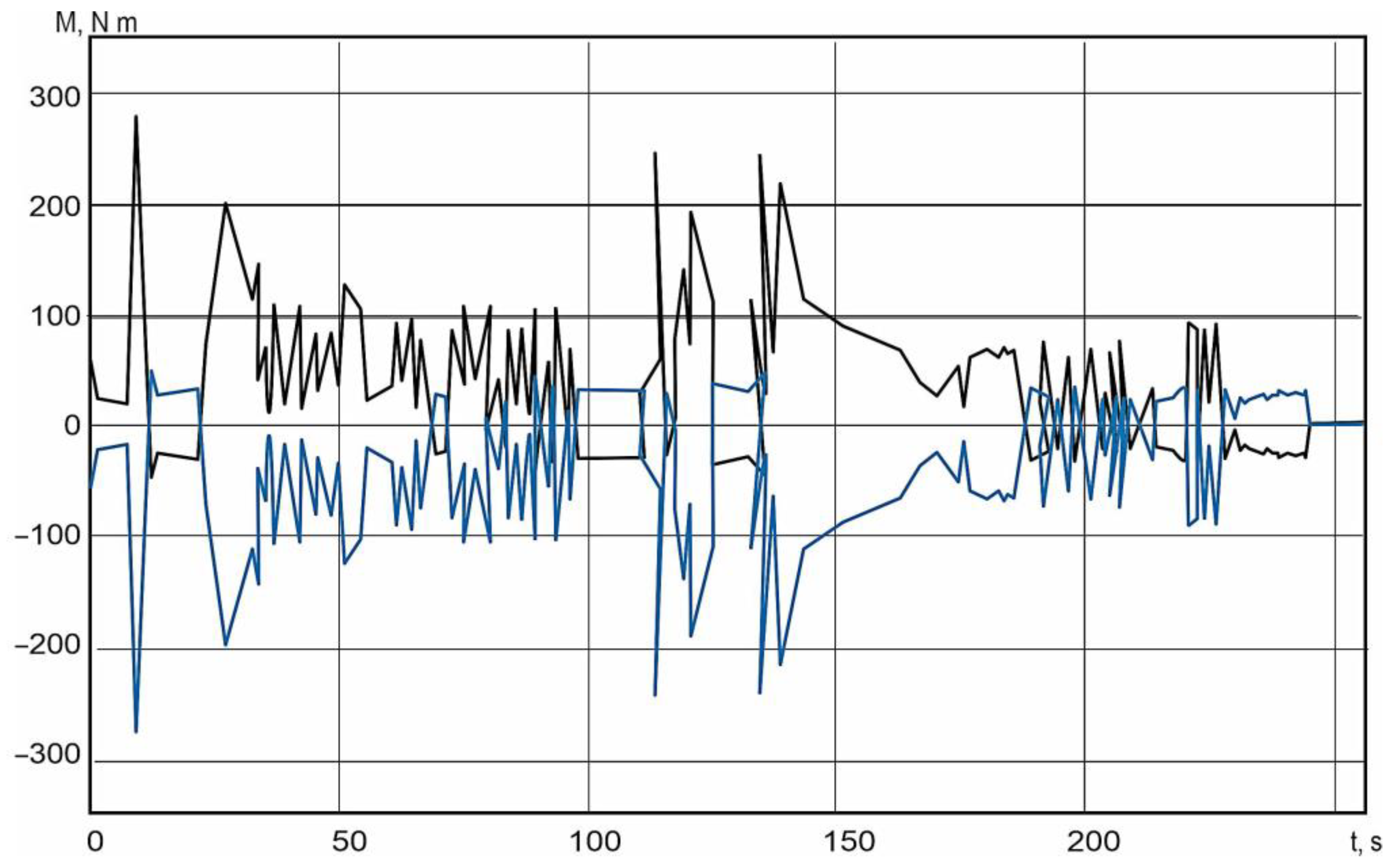
Figure 28 shows the oscillograms of motor torques when moving in a given cycle.

Figure 28.
Motor torque graph obtained from the experimental study: black line—engine torque; purple line—resistance torque.
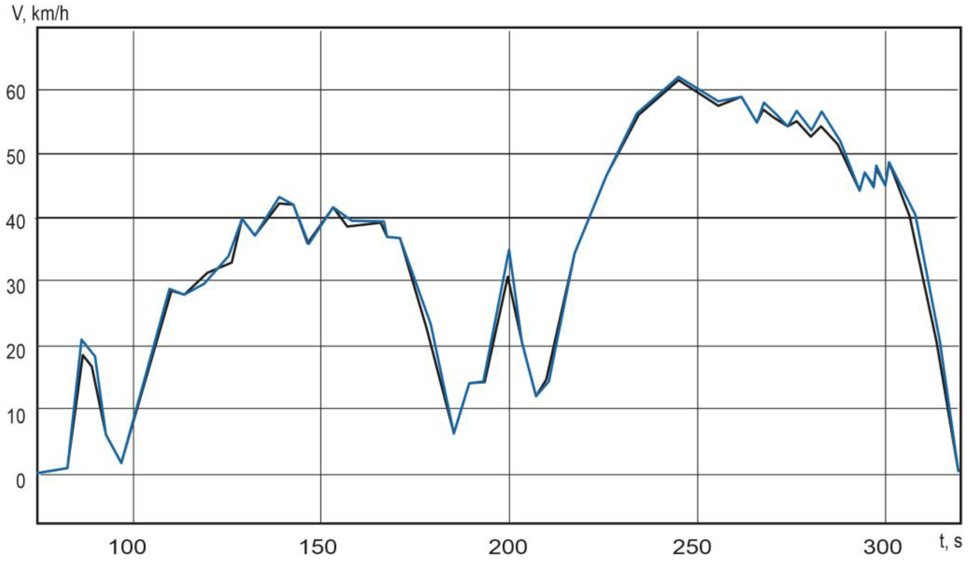
To verify the model, the sum of torques of the electric motors measured under experimental conditions (Figure 27) is input to the car dynamics calculation block (Figure 25). During the first run of the model, without taking into account the moments of inertia of the vehicle coupling mechanisms, the cycle speed was significantly higher than the simulation speed (Figure 29).
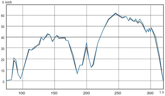
Figure 29.
Comparison of electric vehicle speeds in simulation and real tests: black line—simulation movement; blue line—real car movement.
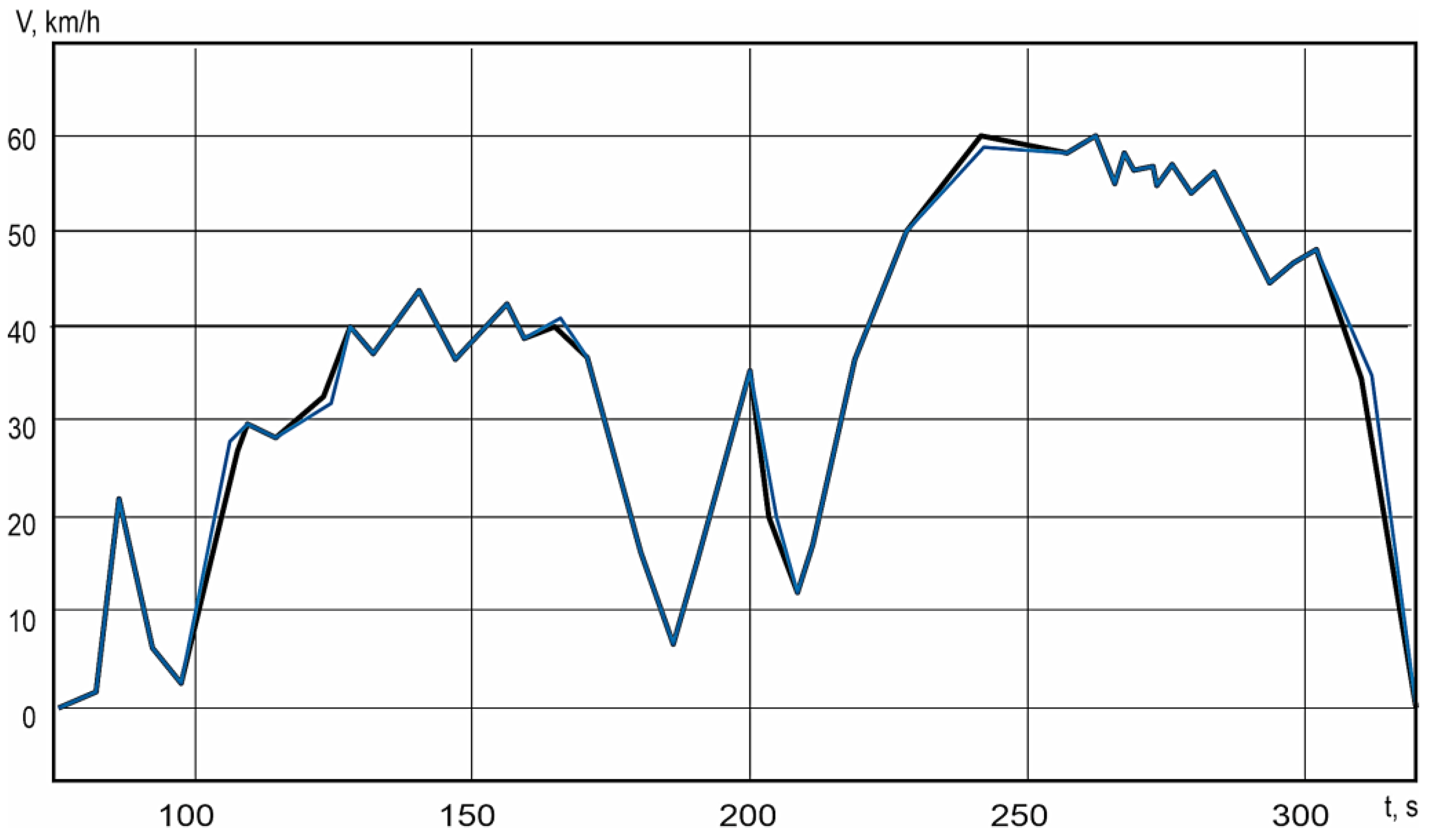
After comparing the results, the value of the moment of inertia was corrected to take into account the rotating masses of the gears used in the electric portal bridge [21,64]. After running the mathematical model again, the graph in the acceleration plots matched the values in the test report (Figure 30).
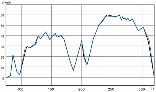
Figure 30.
Comparison of electric vehicle speeds in simulation and real tests, after correction of the moment of inertia: black line—simulation movement; blue line—real car movement.
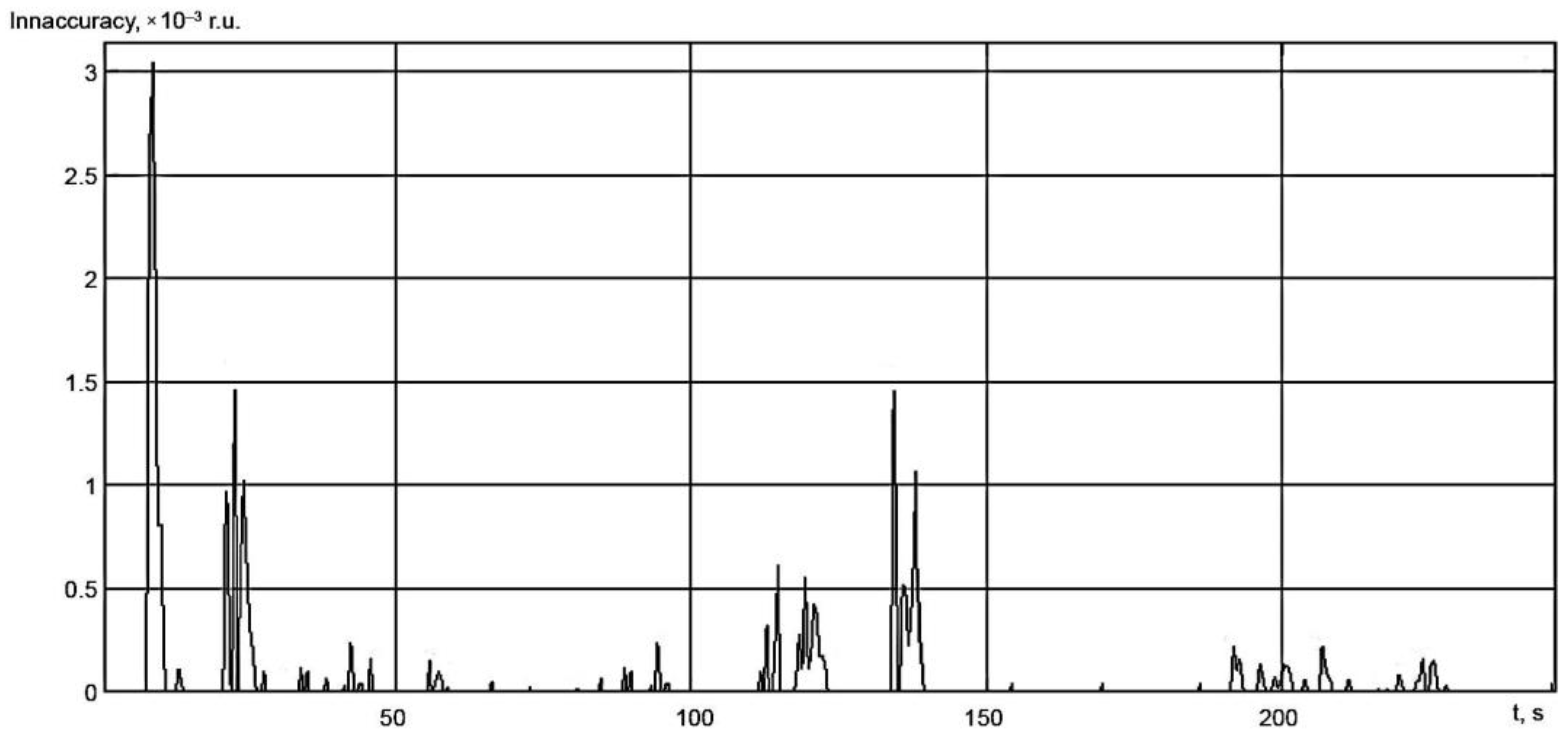
As a result, the maximum error was 0.3% in braking mode. The total error was 0.8%. A graph of errors in the cycle is shown in Figure 31.

Figure 31.
Modelling errors in a motion cycle.
The data obtained from the mechanical model were duplicated in the electrical part, and verification of the mechanical performance with a maximum error of 0.8% was achieved.
5. Checking the Energy Performance of an Electric Vehicle
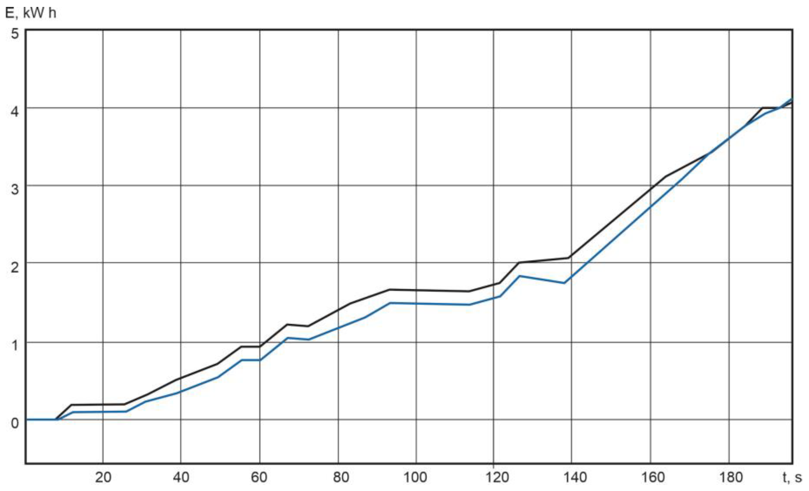
The energy consumption in real tests with the CAN protocol was 1.69 kWh/km. In order to compare the obtained consumption data, it is necessary to perform mathematical modelling on the driving cycle [65]. Since energy recovery is limited and the standard braking system, together with regeneration, was applied during driving, the verification of energy consumption would not be reliable. Therefore, to compare the energy performance, it is necessary to compare the energy expended without regeneration [66].
The value of battery energy consumption measured in a cycle was 4.4 kWh. The same parameter obtained by mathematically modelling the vehicle movement without energy recovery was 4.48 kWh. The difference is due to the fact that, during stopping and braking, the battery current in the mathematical model is not equal to zero. An alignment of the obtained values of battery energy without regeneration in real tests and the simulation in the driving cycle is shown in Figure 32.
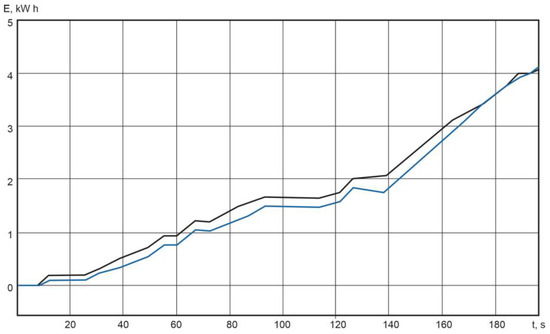
Figure 32.
Matching battery energy without considering regeneration in real tests and in driving cycle: black line—simulation movement; blue line—real car movement.
The graph shows the discrepancy between the real tests and the modelling of the system in the middle of the cycle; this is due to taking into account the needs of the electric vehicle, as well as the operation of the compressor of the pneumatic system [67].
The results obtained allow us to obtain energy characteristics, not only in driving cycles measured as a result of experimental studies, but also to calculate characteristics in standardised driving cycles with maximum reliability [68].
6. Verification of Speed Characteristics with Test Report
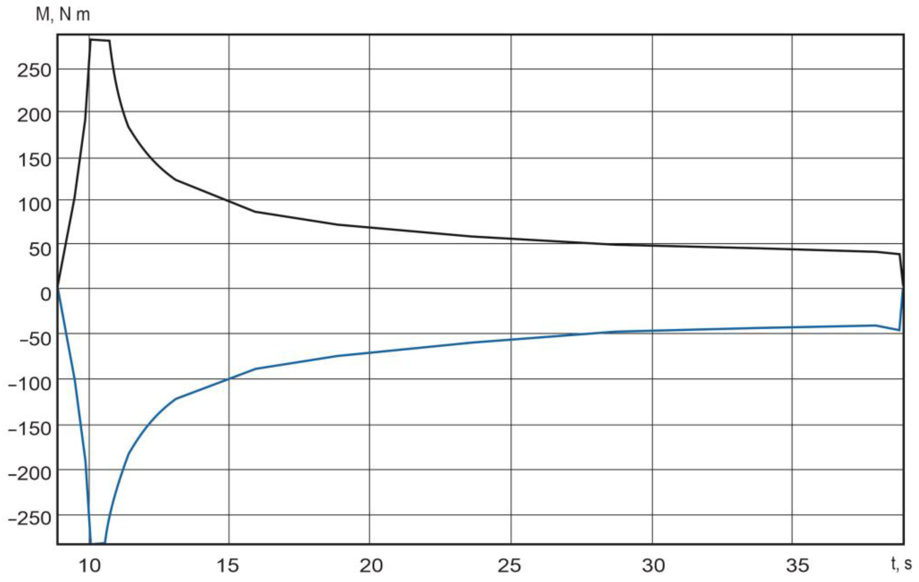
According to the tests carried out, the acceleration of the electric car to 60 km/h is 33.8 s. To verify the acceleration, an external motor characteristic is required. Taking into account that the motors do not operate in the optimal range of battery voltage and the external characteristics given in the specification cannot be realised, it is necessary to obtain the external characteristic from the acceleration tests of the electric car. A family of external characteristics is obtained from the tests of the electric vehicle at individual modes. To investigate the acceleration characteristic, the external characteristic obtained at a battery charge level of 35% was used in the simulation. The other characteristics were not analysed due to the fact that the measurements were carried out on the sections with descents and ascents. The obtained external characteristic is shown in Figure 33.

Figure 33.
External characteristic obtained from testing an electric vehicle: black line—engine torque; blue line—resistance torque.
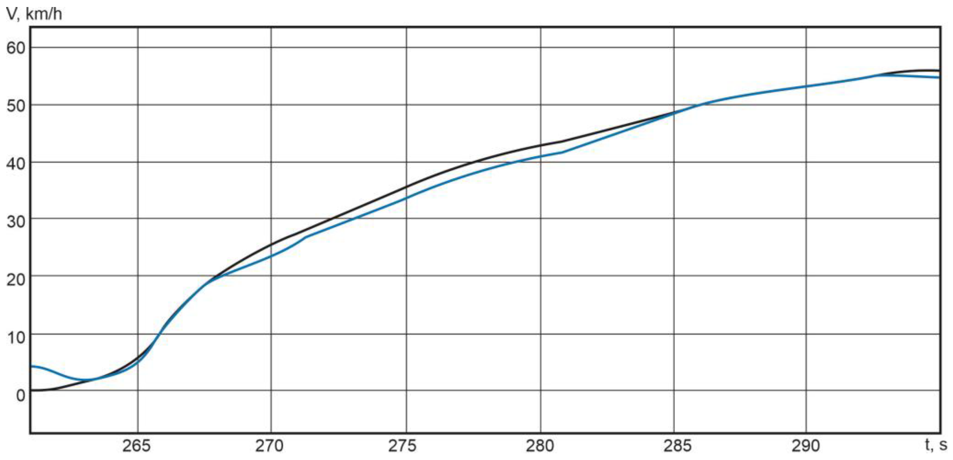
The torque signal of the external velocity response is input to the mechanical model. This compares the velocities over the motion cycle and the simulation velocity (Figure 34).

Figure 34.
Experimental estimation of velocities in a motion cycle: black line—simulation movement; blue line—real car movement.
According to the simulation results, the acceleration to a speed of 58 km/h was 30 s. Taking into account the battery discharge and the limitations applied in the electric vehicle, the difference of 0.1 s can be considered acceptable.
The experimental data obtained during the operation of the electric vehicle indicate a low voltage level of the battery. This is due to the layout solutions that were used to accommodate the lithium–titanate battery. In cases of the application of promising technologies, it is possible to achieve a voltage level of 650 V and more, which will facilitate increasing traction currents for this type of electric drive, without reducing the traction-dynamic characteristics. A comparison of the characteristics obtained during the modelling of the electric vehicle in peak and recommended modes shows a significant improvement in the energy performance of the battery.
7. Conclusions
The performance characteristics of the battery pack while driving a Mitsubishi MIEV electric vehicle were obtained. Measurements were made using CAN technology in different electric vehicle weight and road conditions. As a result, it was determined that the electric lorry could drive two complete cycles on a route. In the case of advanced technologies, it is possible to achieve higher voltage levels on the traction batteries of the electric vehicle. Such batteries will facilitate an increase in the traction current for this type of electric drive, without reducing the traction–dynamic characteristics. A comparison of the characteristics obtained when modelling the electric vehicle in peak and recommended modes shows a significant improvement in the energy performance of the batteries. The obtained graphs of currents in the nominal driving mode can be used for further calculations of battery life and thermal characteristics.
A complex mathematical model of an electric vehicle including a traction battery, two inverters and two induction motors integrated into an electric portal bridge was developed. It is shown that the developed mathematical model can be used to calculate the load parameters of the battery in standardised driving cycles.
The energy consumption in the actual test with the CAN protocol was 1.69 kWh/km. The value of battery energy consumption measured per cycle was 4.4 kWh. The same parameter obtained by mathematically modelling the vehicle movement without energy recovery was 4.48 kWh. The obtained results allow us to obtain energy characteristics, not only in driving cycles measured as a result of experimental studies, but also to calculate the characteristics in standardised driving cycles. An induction motor was chosen because asynchronous models have a simpler design and more reliable operation, and they are cheaper. The cost of synchronous motors is higher than that of asynchronous motors, which makes it less profitable to equip electric or hybrid cars with them. The use of modern PWM controllers makes the induction motor promising for use in electric cars.
A verification of the data was carried out by comparing the data from EN 1986-1:1997, “Electrically propelled road vehicles—Measurement of energy performances” with the results of our mathematical modelling.
Author Contributions
Conceptualization, B.V.M. and N.V.M.; methodology, S.N.S. and E.A.E.; software, M.Q.; validation, S.N.S. and E.A.E.; formal analysis, S.N.S. and E.A.E.; investigation, D.V.V.; resources, D.V.V.; data curation, D.V.V.; writing—original draft preparation, B.V.M. and N.V.M.; writing—review and editing, B.V.M. and N.V.M.; visualization, M.Q. All authors have read and agreed to the published version of the manuscript.
Funding
This research received no external funding.
Data Availability Statement
No new data were created or analyzed in this study. Data sharing is not applicable to this article.
Conflicts of Interest
The authors declare no conflicts of interest.
References
- Zhao, L.; Wang, Z.; Feng, J.; Zheng, S.; Ning, X. Construction Method for Reliability Test Driving Cycle of Electric Vehicle Drive System Based on Users’ Big Data. J. Mech. Eng. 2021, 57, 129–140. [Google Scholar] [CrossRef]
- Bilal, M.; Rizwan, M.; Alsaidan, I.; Almasoudi, F. AI-based Approach for Optimal Placement of EVCS and DG with Reliability Analysis. IEEE Access 2021, 9, 154204–154224. [Google Scholar] [CrossRef]
- Gandoman, F.H.; Emad, A.; Ziad, A.; Maitane, B.; Zobaa, A.; Shady, A.A. Reliability Evaluation of Lithium-Ion Batteries for E-Mobility Applications from Practical and Technical Perspectives: A Case Study. Sustainability 2021, 13, 11688. [Google Scholar] [CrossRef]
- Ghosh, A.; Erickson, R.W. Drive Cycle Based Reliability Analysis of Composite DC-DC Converters for Electric Vehicles. In Proceedings of the 2020 IEEE Transportation Electrification Conference & Expo (ITEC), Virtual, 22–26 June 2020; pp. 544–549. [Google Scholar] [CrossRef]
- Charles, R.S.; Vijaya, K.N.M.; Senthil, K.J.; Jeslin, D.N.J. Enhancing system reliability by optimally integrating PHEV charging station and renewable distributed generators: A Bi-Level programming approach. Energy 2021, 229, 120746. [Google Scholar]
- Waldmann, T.; Kasper, M.; Fleischhammer, M.; Wohlfahrt-Mehrens, M. Temperature dependent aging mechanisms in Lithium-Ion batteries-A Post-Mortem study. J. Power Sources 2014, 363, 129–135. [Google Scholar] [CrossRef]
- Casals, L.C.; Martinez-Laserna, E.; García, B.A.; Nieto, N. Sustainability analysis of the electric vehicle use in Europe for CO2 emissions reduction. J. Clean. Prod. 2016, 127, 425–437. [Google Scholar] [CrossRef]
- Filina, O.A.; Tynchenko, V.S.; Kukartsev, V.A.; Bashmur, K.A.; Pavlov, P.P.; Panfilova, T.A. Increasing the Efficiency of Diagnostics in the Brush-Commutator Assembly of a Direct Current Electric Motor. Energies 2024, 17, 17. [Google Scholar] [CrossRef]
- Xia, B.; Wang, S.; Tian, Y.; Sun, W.; Xu, Z.; Zheng, W. Experimental study on the linixcoymnzo2 lithium-ion battery characteristics for model modification of SOC estimation. Inf. Technol. J. 2014, 13, 2395–2403. [Google Scholar] [CrossRef]
- Boychuk, I.P.; Grinek, A.V.; Tynchenko, V.S.; Kukartsev, V.A.; Tynchenko, Y.A.; Kondratiev, S.I. A Methodological Approach to the Simulation of a Ship’s Electric Power System. Energies 2023, 16, 8101. [Google Scholar] [CrossRef]
- Li, X.; Jiang, J.; Zhang, C.; Wang, L.Y.; Zheng, L. Robustness of SOC estimation algorithms for EV lithium-ion batteries against modelling errors and measurement noise. Math. Probl. Eng. 2015, 2015, 719490. [Google Scholar]
- Tian, Y.; Xia, B.; Wang, M.; Sun, W.; Xu, Z. Comparison study on two model-based adaptive algorithms for SOC estimation of lithium-ion batteries in electric vehicles. Energies 2014, 7, 8446–8464. [Google Scholar] [CrossRef]
- Tseng, K.-H.; Liang, J.-W.; Chang, W.; Huang, S.-C. Regression models using fully discharged voltage and internal resistance for state of health estimation of lithium-ion batteries. Energies 2015, 8, 2889–2907. [Google Scholar] [CrossRef]
- Kukartsev, V.V.; Gozbenko, V.E.; Konyukhov, V.Y.; Mikhalev, A.S.; Kukartsev, V.A.; Tynchenko, Y.A. Determination of the Reliability of Urban Electric Transport Running Autonomously through Diagnostic Parameters. World Electr. Veh. J. 2023, 14, 334. [Google Scholar] [CrossRef]
- Hafsaoui, J.; Sellier, F. Electrochemical model and its parameters identification tool for the follow-up of battery aging. World Electric. Veh. J. 2010, 4, 386–395. [Google Scholar] [CrossRef]
- Prada, E.; Di Domenico, D.; Creff, Y.; Sauvant-Moynot, V. Towards advanced BMS algorithms development for (p)hev and EV by using a physics-based model of Li-Ion Battery Systems. World Electric. Veh. J. 2013, 6, 807–818. [Google Scholar] [CrossRef]
- Varini, M.; Campana, P.E.; Lindbergh, G. A semi-empirical, electrochemistry-based model for Li-ion battery performance prediction over lifetime. J. Energy Storag. 2019, 25, 100819. [Google Scholar] [CrossRef]
- Ashwin, T.R.; McGordon, A.; Jennings, P.A. Electrochemical modelling of li-ion battery packs with constant voltage cycling. J. Power Sources 2017, 341, 327–339. [Google Scholar] [CrossRef]
- Somakettarin, N.; Pichetjamroen, A. A study on modelling of effective series resistance for lithium-ion batteries under life cycle consideration. IOP Conf. Ser. Earth Environ. Sci. 2019, 322, 012008. [Google Scholar] [CrossRef]
- Kuo, T.J.; Lee, K.Y.; Chiang, M.H. Development of a neural network model for SOH of LiFePO4 batteries under different aging conditions. IOP Conf. Ser. Mater. Sci. Eng. 2019, 486, 012083. [Google Scholar] [CrossRef]
- Lacey, G.; Putrus, G.; Bentley, E. Smart EV charging schedules: Supporting the grid and protecting battery life. IET Electr. Syst. Transp. 2017, 7, 84–91. [Google Scholar] [CrossRef]
- Ilyushin, Y.V.; Pervukhin, D.A.; Afanasieva, O.V.; Afanasyev, M.P.; Kolesnichenko, S.V. Solution of problem of heating elements’ location of distributed control objects. Glob. J. Pure Appl. Math. 2016, 12, 585–602. [Google Scholar]
- Mamun, K.A.; Islam, F.R.; Haque, R.; Chand, A.A.; Prasad, K.A.; Goundar, K.K.; Prakash, K.; Maharaj, S. Systematic Modeling and Analysis of On-Board Vehicle Integrated Novel Hybrid Renewable Energy System with Storage for Electric Vehicles. Sustainability 2022, 14, 2538. [Google Scholar] [CrossRef]
- Chao, P.-P.; Zhang, R.-Y.; Wang, Y.-D.; Tang, H.; Dai, H.-L. Warning model of new energy vehicle under improving time-to-rollover with neural network. Meas. Control. 2022, 55, 1004–1015. [Google Scholar] [CrossRef]
- Pusztai, Z.; Korös, P.; Szauter, F.; Friedler, F. Vehicle Model-Based Driving Strategy Optimisation for Lightweight Vehicle. Energies 2022, 15, 3631. [Google Scholar] [CrossRef]
- Mariani, V.; Rizzo, G.; Tiano, F.; Glielmo, L. A model predictive control scheme for regenerative braking in vehicles with hybridised architectures via aftermarket kits. Control Eng. Pract. 2022, 123, 105142. [Google Scholar] [CrossRef]
- Cordoba, A. Capacity and power fade cycle-life model for plug-in hybrid electric vehicle lithium-ion battery cells containing blended spinel and layered-oxide positive electrodes. J. Power Sources 2015, 278, 473–483. [Google Scholar] [CrossRef]
- Martyushev, N.V.; Malozyomov, B.V.; Filina, O.A.; Sorokova, S.N.; Efremenkov, E.A.; Valuev, D.V.; Qi, M. Stochastic Models and Processing Probabilistic Data for Solving the Problem of Improving the Electric Freight Transport Reliability. Mathematics 2023, 11, 4836. [Google Scholar] [CrossRef]
- Laadjal, K.; Cardoso, A.J.M. Estimation of Lithium-Ion Batteries State-Condition in Electric Vehicle Applications: Issues and State of the Art. Electronics 2021, 10, 1588. [Google Scholar] [CrossRef]
- Arango, I.; Lopez, C.; Ceren, A. Improving the Autonomy of a Mid-Drive Motor Electric Bicycle Based on System Efficiency Maps and Its Performance. World Electric. Veh. J. 2021, 12, 59. [Google Scholar] [CrossRef]
- Volneikina, E.; Kukartseva, O.; Menshenin, A.; Tynchenko, V.; Degtyareva, K. Simulation-Dynamic Modeling of Supply Chains Based On Big Data. In Proceedings of the 2023 22nd International Symposium Infoteh-Jahorina, Infoteh 2023, East Sarajevo, Bosnia and Herzegovina, 15–17 March 2023. [Google Scholar] [CrossRef]
- Wu, X. Research and Implementation of Electric Vehicle Braking Energy Recovery System Based on Computer. J. Phys. Conf. Ser. 2021, 1744, 022080. [Google Scholar] [CrossRef]
- Sorokova, S.N.; Efremenkov, E.A.; Valuev, D.V.; Qi, M. Review Models and Methods for Determining and Predicting the Reliability of Technical Systems and Transport. Mathematics 2023, 11, 3317. [Google Scholar] [CrossRef]
- Domanov, K.; Shatohin, A.; Nezevak, V.; Cheremisin, V. Improving the technology of operating electric locomotives using electric power storage device. E3S Web Conf. 2019, 110, 01033. [Google Scholar] [CrossRef]
- Malozyomov, B.V.; Martyushev, N.V.; Konyukhov, V.Y.; Oparina, T.A.; Zagorodnii, N.A.; Efremenkov, E.A.; Qi, M. Mathematical Analysis of the Reliability of Modern Trolleybuses and Electric Buses. Mathematics 2023, 11, 3260. [Google Scholar] [CrossRef]
- Kral, C.; Haumer, A.; Kubicek, B.; Winter, O. Model of a Squirrel Cage Induction Machine with Interbar Conductances. In Proceedings of the 7th International Modelica Conference, Como, Italy, 20–22 September 2009. [Google Scholar] [CrossRef]
- Liu, X.; Zhao, M.; Wei, Z.; Lu, M. The energy management and economic optimisation scheduling of microgrid based on Colored Petri net and Quantum-PSO algorithm. Sustain. Energy Technol. Assess. 2022, 53, 102670. [Google Scholar] [CrossRef]
- Tormos, B.; Pla, B.; Bares, P.; Pinto, D. Energy Management of Hybrid Electric Urban Bus by Off-Line Dynamic Programming Optimisation and One-Step Look-Ahead Rollout. Appl. Sci. 2022, 12, 4474. [Google Scholar] [CrossRef]
- Zhou, J.; Feng, C.; Su, Q.; Jiang, S.; Fan, Z.; Ruan, J.; Sun, S.; Hu, L. The Multi-Objective Optimisation of Powertrain Design and Energy Management Strategy for Fuel Cell-Battery Electric Vehicle. Sustainability 2022, 14, 6320. [Google Scholar] [CrossRef]
- Semenova, E.; Tynchenko, V.; Chashchina, S.; Suetin, V.; Stashkevich, A. Using UML to Describe the Development of Software Products Using an Object Approach. In Proceedings of the 2022 IEEE International IOT, Electronics and Mechatronics Conference, IEMTRONICS 2022, Toronto, ON, Canada, 1–4 June 2022. [Google Scholar] [CrossRef]
- Sorokova, S.N.; Efremenkov, E.A.; Qi, M. Mathematical Modeling the Performance of an Electric Vehicle Considering Various Driving Cycles. Mathematics 2023, 11, 2586. [Google Scholar]
- Ehsani, M.; Wang, F.-Y.; Brosch, G.L. (Eds.) Transportation Technologies for Sustainability; Springer: New York, NY, USA, 2013. [Google Scholar]
- Voitovich, E.V.; Kononenko, R.V.; Konyukhov, V.Y.; Tynchenko, V.; Kukartsev, V.A.; Tynchenko, Y.A. Designing the Optimal Configuration of a Small Power System for Autonomous Power Supply of Weather Station Equipment. Energies 2023, 16, 5046. [Google Scholar] [CrossRef]
- Sorokova, S.N.; Efremenkov, E.A.; Qi, M. Mathematical Modeling of Mechanical Forces and Power Balance in Electromechanical Energy Converter. Mathematics 2023, 11, 2394. [Google Scholar] [CrossRef]
- Raugei, M.; Hutchinson, A.; Morrey, D. Can electric vehicles significantly reduce our dependence on non-renewable energy? Scenarios of compact vehicles in the UK as a case in point. J. Clean. Prod. 2018, 201, 1043–1051. [Google Scholar] [CrossRef]
- Xia, Q.; Wang, Z.; Ren, Y.; Sun, B.; Yang, D.; Feng, Q. A reliability design method for a lithium-ion battery pack considering the thermal disequilibrium in electric vehicles. J. Power Sources 2018, 386, 10–20. [Google Scholar] [CrossRef]
- Balagurusamy, E. Reliability Engineering, First, P-24, Green Park Extension; McGraw Hill Education (India) Private Limited: New Delhi, India, 2002. [Google Scholar]
- Malozyomov, B.V.; Martyushev, N.V.; Kukartsev, V.V.; Tynchenko, V.S.; Bukhtoyarov, V.V.; Wu, X.; Tyncheko, Y.A.; Kukartsev, V.A. Overview of Methods for Enhanced Oil Recovery from Conventional and Unconventional Reservoirs. Energies 2023, 16, 4907. [Google Scholar] [CrossRef]
- Khalikov, I.H.; Kukartsev, V.A.; Kukartsev, V.V.; Tynchenko, V.S.; Tynchenko, Y.A.; Qi, M. Review of Methods for Improving the Energy Efficiency of Electrified Ground Transport by Optimizing Battery Consumption. Energies 2023, 16, 729. [Google Scholar]
- Aggarwal, K.K. Maintainability and Availability, Topics in Safety Reliability and Quality; Springer: Dordrecht, The Netherlands, 1993. [Google Scholar]
- Shu, X.; Guo, Y.; Yang, W.; Wei, K.; Zhu, Y.; Zou, H. A Detailed Reliability Study of the Motor System in Pure Electric Vans by the Approach of Fault Tree Analysis. IEEE Access 2020, 8, 5295–5307. [Google Scholar] [CrossRef]
- Klyuev, R.V.; Dedov, S.I. Determination of Inactive Powers in a Single-Phase AC Network. Energies 2021, 14, 4814. [Google Scholar] [CrossRef]
- Klyuev, R.V.; Andriashin, S.N. Degradation of Lithium-Ion Batteries in an Electric Transport Complex. Energies 2021, 14, 8072. [Google Scholar] [CrossRef]
- Kukartsev, V.A.; Kukartsev, V.V.; Tynchenko, S.V.; Klyuev, R.V.; Zagorodnii, N.A.; Tynchenko, Y.A. Study of Supercapacitors Built in the Start-Up System of the Main Diesel Locomotive. Energies 2023, 16, 3909. [Google Scholar] [CrossRef]
- Xia, Q.; Wang, Z.; Ren, Y.; Tao, L.; Lu, C.; Tian, J.; Hu, D.; Wang, Y.; Su, Y.; Chong, J.; et al. A modified reliability model for lithium-ion battery packs based on the stochastic capacity degradation and dynamic response impedance. J. Power Sources 2019, 423, 40–51. [Google Scholar] [CrossRef]
- Isametova, M.E.; Nussipali, R.; Martyushev, N.V.; Malozyomov, B.V.; Efremenkov, E.A.; Isametov, A. Mathematical Modeling of the Reliability of Polymer Composite Materials. Mathematics 2022, 10, 3978. [Google Scholar] [CrossRef]
- Bolvashenkov, I.; Herzog, H.-G. Approach to predictive evaluation of the reliability of electric drive train based on a stochastic model. In Proceedings of the 2015 International Conference on Clean Electrical Power (ICCEP), Taormina, Italy, 16–18 June 2015; pp. 486–492. [Google Scholar]
- Ammaiyappan, B.S.; Ramalingam, S. Reliability investigation of electric vehicles. Life Cycle Reliab. Saf. Eng. 2019, 8, 141–149. [Google Scholar] [CrossRef]
- Khalilzadeh, M.; Fereidunian, A. A Markovian approach applied to reliability modelling of bidirectional DC-DC converters used in PHEVs and smart grids. IJEEE 2016, 12, 301–313. [Google Scholar]
- Kheradmand-Khanekehdani, H.; Gitizadeh, M. Well-being analysis of distribution network in the presence of electric vehicles. Energy 2018, 155, 610–619. [Google Scholar] [CrossRef]
- Sadeghian, O.; N-Heris, M.; Abapour, M.; Taheri, S.S.; Zare, K. Improving reliability of distribution networks using plug-in electric vehicles and demand response. J. Mod. Power Syst. Clean Energy 2019, 7, 1189–1199. [Google Scholar] [CrossRef]
- Galiveeti, H.R.; Goswami, A.K.; Choudhury, N.B.D. Impact of plug-in electric vehicles and distributed generation on reliability of distribution systems. Eng. Sci. Technol. Int. J. 2018, 21, 50–59. [Google Scholar] [CrossRef]
- Garcés Quílez, M.; Abdel-Monem, M.; El Baghdadi, M.; Yang, Y.; Van Mierlo, J.; Hegazy, O. Modelling, Analysis and Performance Evaluation of Power Conversion Units in G2V/V2G Application-A Review. Energies 2018, 11, 1082. [Google Scholar] [CrossRef]
- Yelemessov, K.; Sabirova, L.B.; Bakhmagambetova, G.B.; Atanova, O.V. Modeling and Model Verification of the Stress-Strain State of Reinforced Polymer Concrete. Materials 2023, 16, 3494. [Google Scholar] [CrossRef] [PubMed]
- Kasturi, K.; Nayak, C.K.; Nayak, M.R. Electric vehicles management enabling G2V and V2G in smart distribution system for maximizing profits using MOMVO. Int. Trans. Electr. Energy Syst. 2019, 29, e12013. [Google Scholar] [CrossRef]
- Billinton, R.; Allan, R.N. Reliability Evaluation of Engineering Systems; Springer: Boston, MA, USA, 1992. [Google Scholar]
- Malozyomov, B.V.; Kukartsev, V.V.; Martyushev, N.V.; Kondratiev, V.V.; Klyuev, R.V.; Karlina, A.I. Improvement of Hybrid Electrode Material Synthesis for Energy Accumulators Based on Carbon Nanotubes and Porous Structures. Micromachines 2023, 14, 1288. [Google Scholar] [CrossRef]
- Sorokova, S.N.; Efremenkov, E.A.; Qi, M. Mathematical Modeling of the State of the Battery of Cargo Electric Vehicles. Mathematics 2023, 11, 536. [Google Scholar] [CrossRef]
- Baranovskyi, D.; Bulakh, M.; Michajłyszyn, A.; Myamlin, S.; Muradian, L. Determination of the Risk of Failures of Locomotive Diesel Engines in Maintenance. Energies 2023, 16, 4995. [Google Scholar] [CrossRef]
- De Santis, M.; Silvestri, L.; Forcina, A. Promoting electric vehicle demand in Europe: Design of innovative electricity consumption simulator and subsidy strategies based on well-to-wheel analysis. Energy Convers. Manag. 2022, 270, 116279. [Google Scholar] [CrossRef]
- Pollák, F.; Vodák, J.; Soviar, J.; Markovič, P.; Lentini, G.; Mazzeschi, V.; Luè, A. Promotion of Electric Mobility in the European Union-Overview of Project PROMETEUS from the Perspective of Cohesion through Synergistic Cooperation on the Example of the Catching-Up Region. Sustainability 2021, 13, 1545. [Google Scholar] [CrossRef]


Disclaimer/Publisher’s Note: The statements, opinions and data contained in all publications are solely those of the individual author(s) and contributor(s) and not of MDPI and/or the editor(s). MDPI and/or the editor(s) disclaim responsibility for any injury to people or property resulting from any ideas, methods, instructions or products referred to in the content. |
© 2024 by the authors. Licensee MDPI, Basel, Switzerland. This article is an open access article distributed under the terms and conditions of the Creative Commons Attribution (CC BY) license (https://creativecommons.org/licenses/by/4.0/).