Moving Discretized Control Set Model Predictive Control with Dominant Parameter Identification Strategy for Dual Active Bridge Converters

Abstract

The dual active bridge (DAB) converter has grown significantly as one of the most important units for energy distribution, connecting various types of renewable energy sources with the DC microgrid. For controlling the DAB converter, moving discretized control set model predictive control (MDCS-MPC) is considered one of the most effective methods because of its advantages, such as high dynamic performance and multiobjective control. However, MDCS-MPC strongly depends on the accuracy of system parameters. Meanwhile, the system parameters can be changed due to temperature drift, manufacturing tolerance, age, and operating circumstances. As a result, the steady-state performance of the output voltage of MDCS-MPC is affected. Motivated by this, this paper proposes MDCS-MPC combined with the parameter identification technique to improve the steady-state performance of the output voltage of the DAB converter. Then, analysis of the percentage of the steady-state error of the output voltage is defined on six model parameters, and sensitivity analysis of two dominant parameters is chosen. After that, a straightforward least-squares analysis (LSA) technique is used to identify the two parameters online. The proposed method is verified through simulation in several different operating scenarios to verify its effectiveness.

1. Introduction

As the demand for electrical applications continues to rise, the DC microgrid has experienced a rapid expansion in recent years. Along with this, the bidirectional DC–DC converters are the fundamental units of the DC microgrid. Using these converters to interlink various renewable energy sources with the DC bus and between the various voltage levels available in DC microgrids is common practice. In energy distribution, many renewable energy sources are connected to energy storage systems (ESSs) and solid-state transformers (SSTs). Because of this, the fundamental functions of DC–DC converters are regulating voltage and current and transferring power in both directions. Despite this, these tasks provide several issues that need more academic and industrial attention [1,2,3,4,5,6].

According to [2], several different topologies for bidirectional DC–DC converters have been investigated and proposed. Among them, the dual active bridge (DAB) converter, as shown in Figure 1, is considered one of the potential typologies for the applications of SSTs and ESSs [7]. These statements are for the following reasons: (1) The DAB converter is built with modular capabilities, symmetric structures, and adjustable phase shift modulations, enabling it to change the power flow direction automatically. As a result, the DAB converter is appropriate for applications that include SSTs and ESSs connecting with DC microgrid. (2) It is essential to have a high voltage and current conversion gain to interface ESSs like batteries and supercapacitors, which might undergo significant changes depending on the state of charge (SOC). In addition, a high voltage and current conversion gain converter is required to complete the connection between the pulsed power loads and the power sources. (3) It is possible to attain a wide zero-voltage switching (ZVS) range by utilizing a variety of phase-shift modulations and advanced control and optimization approaches, ultimately resulting in excellent power efficiency [2,6].

For modulation approaches used for transferring the power of the DAB converter, the phase-shift modulation approaches can be categorized as single phase-shift (SPS), extended phase-shift (EPS), dual phase-shift (DPS), and triple phase-shift (TPS).

Table 1. Comparison of modulation.

Modulation	Control Degree	Advantage	Disadvantage
SPS	1	- Easy for implementation - Most widely used	- High circulating power - Limited ZVS range - High current stress
EPS	2	- Low circulating power - Wide ZVS range - Low current stress	- Require one inner phase-shift ratio compared to SPS - The operating states of the two bridges change in the voltage conversion states or changing power flow directions
DPS	2	- Low circulating power - Wide ZVS range - Low current stress	- Require one inner phase-shift ratio compared to SPS
TPS	3	- Low circulating power - Wide ZVS range - Low current stress - High efficiency - Most regulating flexibility	- Require two inner phase-shift ratios compared to SPS - Most complicated for implementation

shows the comparison of modulation. These designations are based on the number and kinds of phase-shift ratios that the modulation approaches use. Compared with EPS, DPS, and TPS, the SPS is the modulation utilized most frequently due to its simplicity by using only one phase-shift ratio as the control variable [1,2,3,4,5,6]. Therefore, this paper utilizes the SPS to show the proposed method’s effectiveness.

Numerous advanced control methods are proposed for the DAB converter, according to [3], such as linearization control [8], output current feedforward control [9], virtual direct power control [10], disturbance observer-based control [11,12,13], feedforward current control [14], predictive current control [15,16], and sliding mode control [17,18,19]. These control strategies have the potential to stabilize and increase the steady-state performance of the output voltage while simultaneously ensuring high dynamics. Compared to other advanced methods, moving discretized control set model predictive control (MDCS-MPC) is frequently considered in power electronics converters due to its numerous benefits, including fast dynamics, easy inclusion of constraints in the cost function, and multiobjective control [20,21,22,23,24].

Table 2. Comparison of the control method.

Control Method	Advantage	Disadvantage
Linearization control	- Easy implementation - Require few sensors	- Low performance
Output current feedforward control	- High performance	- Affected by parameter variation
Virtual direct power control	- High performance	- Affected by parameter variation
Disturbance observer-based control	- Robust against parameter variation - High performance	- Require model information
Feedforward current control	- High performance	- Difficult implementation
Predictive current control	- High performance	- Affected by parameter variation
Sliding mode control	- Easy implementation	- Low performance - Chattering phenomenon
MDCS-MPC	- High performance - Optimization constraint - Multiobjective control	- Difficult implementation

shows the comparison of the control method, according to [1,2,3,4,5,6].

Even though all of the advanced control methods have excellent dynamic performance, they are highly dependent on the accuracy of the system model, which results in a degradation in the steady-state performance if there is a mismatch of the system parameters. This limitation is because the controller’s information usually differs from the hardware’s. In experiments, the values of system parameters such as inductor and capacitor might somewhat shift over time [25,26] due to temperature drift, manufacturing tolerance, age, and operating circumstances; as a result, parameter mismatches of up to 20% can sometimes be observed [27,28]. Therefore, if the system parameters are identified online accurately while the operation is carried out, the steady-state performance significantly improves.

In order to overcome the effect of parameter mismatch, MPC with complex multiobjective optimization control is used in [29] to control the power converter or produce a feed-forward compensator in [30] for a programmable logic controller system. However, they are complicated. On the other hand, to identify parameters online, a model-based feed-forward control strategy combined with recursive least-squares (RLS) is proposed in [31], and a model predictive control with a novel parameter identification scheme of RLS in [32]. However, they do not consider other parameters, such as capacitors. Another method for calculating the parameters presented in [33] can use gradient calculation of the least-squares error function. This technique can identify the actual values using the MPC combined with the least-squares estimate method. However, the least-squares solution presented in [33] with the matrix belonging to ${ℝ}^{3\times 3}$ results in a complicated calculation. In addition, it involves previously and currently measured data, resulting in degraded dynamic performance, as mentioned in [31]. On the other hand, identifying the parameters of the transformer may also be accomplished through the instantaneous phasor method [34] and RLS-based parasitic parameter extraction [35]. However, these control strategies cannot determine capacitor value on both sides of the DAB converter, and their algorithm is also complicated.

Based on those mentioned above, this paper proposes a method for enhancing the steady-state performance of the DAB converter with MDCS-MPC control. At the same time, the system parameters are identified online to eliminate the effects of mismatch. Firstly, sensitivity analyses are carried out for system parameters and the other measured parameters to determine how each parameter impacts the steady-state performance of the converter. After that, the online parameter identification technique is carried out to track the most vital parameters using least-squares analysis (LSA), which is considered the most straightforward technique to find the optimal solution of the linear equation set, according to [36]. The contributions of this research can be summarized as follows:

• The percentages of steady-state error for major system parameters and measurement parameters of the DAB converter are first modeled mathematically. Based on this, a comparison of the percentages of steady-state error is implemented, showing that system parameters $L$ and $C_2$ have the most effect on the output voltage compared to the other parameters. In addition, the effects of system parameters $L$ and $C_2$ are compared in depth through sensitivity analysis by the partial derivative-based method. Then, through simulation verification, the MDCS-MPC shows that it is adversely affected by a mismatch in the system parameters. Simulation results show that the mathematical model is consistent with those in theory, demonstrating the correction of the mathematical model and those in sensitivity analysis.
• A simple parameter identification technique with the LSA is proposed to identify the DAB converter’s actual values of system parameters. After that, by applying their actual values in the MDCS-MPC, the steady-state performance of the output voltage is significantly improved. Moreover, the MDCS-MPC under the match parameters is compared to the proportional–integral (PI) control to show its effectiveness.

The outline of the paper consists of seven sections. In Section 2, the operation principle of the DAB converter under SPS modulation is shown. In Section 3, a brief review of the operating principle of the MDCS-MPC method is presented for perusal. Section 4 discusses and analyzes the analysis of the parameter effects on the steady-state performance and sensitivity analysis of the system parameters of the DAB converter. Section 5 presents the parameter identification technique of the LSA. Simulation results of the DAB converter under different operating scenarios are carried out to show the proposed method’s benefit in Section 6. Finally, the conclusions of the method are presented in Section 7.

2. Operation Principle of the DAB Converter

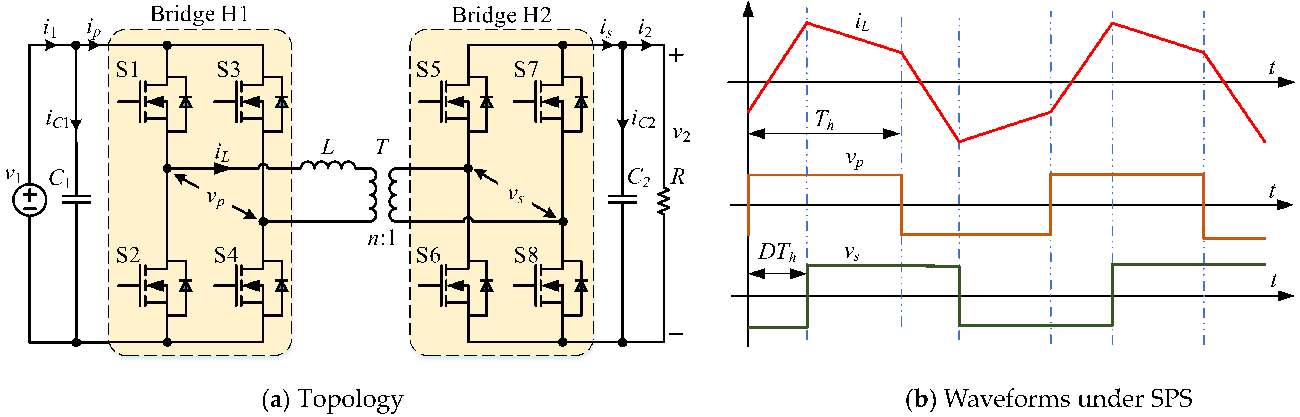
Figure 1a shows the topology of the DAB converter. Assume that the high-frequency transformer T has a turns ratio of n:1, and the power is transferred from the left to the right. The input and output sides are connected to capacitors $C_1$ and $C_2$, respectively. The inductance, denoted by $L$, includes the transformer’s leakage inductance and series inductance. Figure 1b shows the waveforms produced by the DAB converter when subjected to SPS modulation. Therefore, the power transmission between the two bridges is accomplished with a phase-shift ratio of $D$. The switching frequency is denoted by $f,$ while T_h represents the half-switching period.

Several comprehensive modeling research studies on DAB converters can be found in [37,38,39]. Considering that, the DAB converter is regarded as a first-order system. Compared to other models, such as the enhanced reduced-order model [40], the generalized average model [41], and the discrete-time model [42], the reduced-order model [37,43] has been demonstrated to be an excellent middle ground among complexity, flexibility, and accuracy. Reference [3] contains additional information regarding comparing various DAB models. Because of this, the reduced-order model will be applied repeatedly throughout this study. Thus, the current $i_s$ can be represented as follows when the converter is in the steady state

$$i_s=\frac{n{v}_1}{2fL}D\left(1-D\right).$$

(1)

According to (1), it is easy to see that the transferred power will be through the converter when $0\le D\le 1$. The transferred power has a maximum value when $D=0.5$. Thus, from Figure 1, the output current can be obtained as follows

$$C_2\frac{d{v}_2}{dt}=i_s-i_2.$$

(2)

On the other hand, to implement the system model dynamically into the digital signal processor (DSP) easily, the approximation of the first-order derivative can be utilized. Compared to central approximation, backward and forward approximations are straightforward to implement. Thus, the forward approximation is used to discretize (2) as follows [21]

$$v_2\left[k+1\right]=v_2\left[k\right]+\frac{i_s\left[k\right]-i_2\left[k\right]}{f{C}_2}$$

(3)

where $v_2\left[k+1\right]$ and $v_2\left[k\right]$ are the output voltages at the (k + 1)th and kth sampling step, respectively. $i_s\left[k\right]$ and $i_2\left[k\right]$ are the bridge output current and converter output current at the kth sampling step, respectively.

Assuming that there is not a significant change in the load current during one sampling period, this results in

$$i_2\left[k\right]=i_2\left[k+1\right].$$

(4)

Thus, the prediction of the output voltage at the (k + 1)th sampling step is as follows

$$v_2\left[k+2\right]=v_2\left[k+1\right]+\frac{i_s\left[k+1\right]-i_2\left[k\right]}{f{C}_2}.$$

(5)

Substituting $v_2\left[k+2\right]$ into (3)–(5), (6) is obtained as follows

$$v_2\left[k+2\right]=v_2\left[k\right]+\frac{i_s\left[k+1\right]+i_s\left[k\right]-2i_2\left[k\right]}{f{C}_2}.$$

(6)

3. Review of Moving Discretized Control Set Model Predictive Control (MDCS-MPC)

In this section, the operating principle of MDCS-MPC will be briefly summarized from [20,21,22,23,24]. Considering the delay computation, MDCS-MPC has a prediction horizon that spans two sampling intervals. As a result, the following cost function is proposed as follows

$$g\left[k\right]=c_1{\left(v_{2r}-v_2\left[k+2\right]\right)}^2+c_2{\left(v_2\left[k+2\right]-v_2\left[k\right]\right)}^2.$$

(7)

In (7), the weighting factor $c_1$ adjusts the output voltage error from the reference value $v_{2r}$, while the weighting factor $c_2$ determines the voltage fluctuation. Obviously, tuning $c_1$ and $c_2$ is intuitively crucial to the performance of the MDCS-MPC. In addition, a relative weighting factor $c$ can be chosen as follows

$$c=\frac{c_1}{c_2}.$$

(8)

In (8), if $c$ is chosen too small, the system cannot always converge. However, if $c$ is chosen too large, the control bandwidth of the controller will be reduced. Actually, selecting weighting factors requires a sequence of trial and error.

For digital control, the phase-shift ratio $D$ must be discretized. The precision of the discretization depends on the control platform being utilized, with the value ${\Delta }_f$ being the finest phase-shift value. As shown in (9), the phase-shift ratio is discretized for simple analysis when the power is transferred in a unidirectional mode

$$D\in \left\{0,{\Delta }_f,2{\Delta }_f,\dots ,0.5\right\}.$$

(9)

Figure 2 shows an intuitive mechanism of the MDCS-MPC method. For example, during the control interval from k to k + 1, the number of points μ = 3 is examined. The discretized control set is $\left\{\delta -{\Delta }_f,\delta ,\delta +{\Delta }_f\right\}$. After every period of sampling, the center point is recalculated. According to Figure 2, the optimal value of $D$, as shown in the red line, is changed from $\delta +{\Delta }_f$ to $\delta +2{\Delta }_f$ when the sampling step evolves from k to k + 1. Thus, the discretized control set continuously progresses within the value range, as shown in (9). Obviously, increasing μ can improve the transition dynamics. However, it also places a significant computational burden on the controller. Thus, an adaptive step is utilized as follows

$$V_{\Delta }=\left\{\begin{array}{cc}\left|v_{2r}-v_2\left[k\right]\right|& \left|v_{2r}-v_2\left[k\right]\right|\le V_m\\ V_m& \left|v_{2r}-v_2\left[k\right]\right|>V_m\end{array}\right.$$

(10)

$${\Delta }_a={\Delta }_f\left(1+\lambda V_{\Delta }\right)$$

(11)

where $V_m$ is the saturated voltage; $\lambda$ is a coefficient determined according to the requirement of transition performance.

A concise summary of the MDCS-MPC operation principle for the DAB converter can be found as follows. Firstly, the evaluation process begins with calculating the adaptive step, as shown in (10) and (11). Once this is completed, the iteration for MDCS-MPC begins with $D$ shifts within the range described in (9). Then, to compare the minimal, cost functions, as shown in (7), are computed with each corrected voltage prediction value, as shown in (6). Finally, the optimal values of $D$ are then used to control the DAB converter through a pulse width modulation generator.

4. Analysis of the Parameter Effects on the Steady-State Performance

As presented in Section 2, six model parameters of the DAB converter, including system parameters ($L$, $C_2$, and $n$) and measurement parameters ($v_1$, $v_2$, and $i_2$), affect the steady-state performance.

First, the mismatch ratios of the inductance ($m_L$) and output capacitance ($m_{C2}$) are defined as shown in (12)

$$\begin{array}{l}{m}_L=\frac{L_{act}}{L}\\ m_{C2}=\frac{C_{2act}}{C_2}\end{array}$$

(12)

where $L_{act}$ and $C_{2act}$ are the actual values of $L$ and $C_2$, respectively.

In the steady state, the average current flowing through the output capacitor is deemed equal to zero. Thus, it is possible to assume that the current $i_s=i_2=v_2/R$ [44]. Consequently, from (1), (12), and the fact that $v_2$ is controlled as $v_2=v_{2r}$, the output voltage according to $m_L$ and $m_{C2}$ is rewritten as follows

$$v_{2,LC2}=\frac{fR{C}_2{m}_L{m}_{C2}{v}_{2r}}{1-m_L+fR{C}_2{m}_L{m}_{C2}}.$$

(13)

From (13), the percentage of steady-state error $\Delta v_{2,LC2}\%$ is derived as follows

$$\Delta v_{2,LC2}\%=\frac{v_{2,LC2}-v_{2r}}{v_{2r}}\times 100\%=\frac{m_L-1}{1-m_L+fR{C}_2{m}_L{m}_{C2}}\times 100\%.$$

(14)

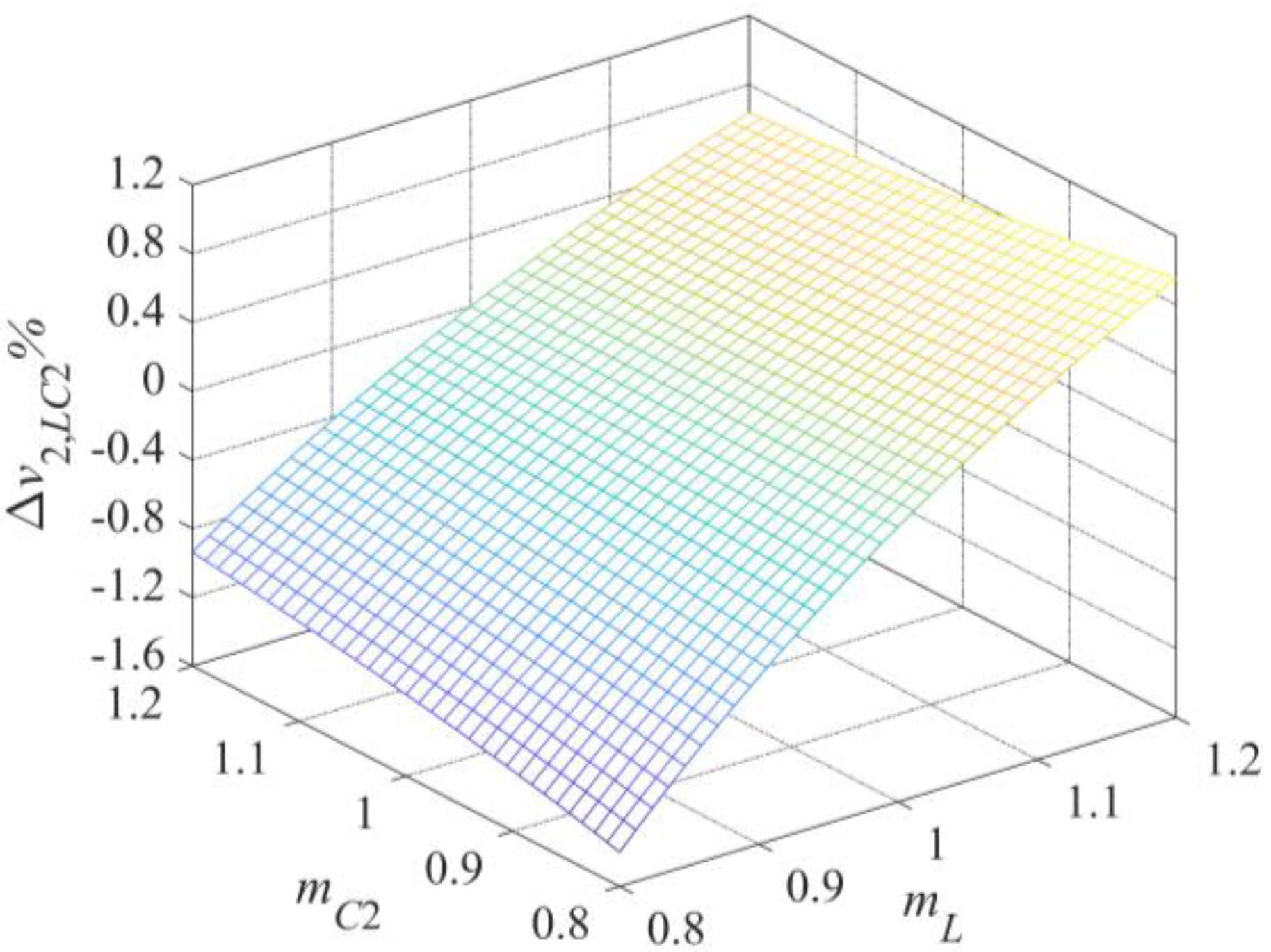
Figure 3 shows the percentage of steady-state error $\Delta v_{2,LC2}\%$ according to $m_L$ and $m_{C2}$. Mismatch ratios $m_L$ and $m_{C2}$ are shown in

Table 3. Range of mismatch ratios.

Mismatch Ratio	Value
$m_L$	±20%
$m_{C2}$	±20%
$m_n$	±0.1%
$m_{v1}$	±0.9%
$m_{i2}$	±0.9%
$m_{v2}$	±0.9%

, considering the maximum mismatches as analyzed in Section 1. The parameters of the converter are shown in

Table 4. System parameters.

Meaning	Symbol	Value
Switching frequency	$f$	10 kHz
Inductance	$L$	50 μH
Input capacitance	$C_1$	440 μF
Output capacitance	$C_2$	220 μF
Input voltage	$v_1$	100 V
Output voltage	$v_2$	80 V
Transformer turn ratio	$n$	1
Resistive load	$R$	10 Ω

. According to Figure 3, $\Delta v_{2,LC2}\%$ has a maximum value of 0.9560% when $m_L$ = 1.2 and $m_{C2}$ = 0.8. On the other hand, $\Delta v_{2,LC2}\%$ shows the minimum value of −1.4006% when $m_L$ = $m_{C2}$ = 0.8. Meanwhile, when $m_L$ = 1, $\Delta v_{2,LC2}\%$ has a value of 0, which means that if $L$ has a perfect match value, $v_2$ has no steady-state error, even if $C_2$ contains mismatches.

Similar to the above analysis, the mismatch ratios of the transformer turn ratio $n$ and input voltage $v_1$ are defined as

$$\begin{array}{l}{m}_n=\frac{n_{act}}{L}\\ m_{v1}=\frac{v_{1act}}{v_1}\end{array}$$

(15)

where $n_{act}$ and $v_{1act}$ are the actual values of n and $v_1$, respectively.

Thus, the output voltage in the steady state is shown as follows

$$v_{2,nv1}=\frac{fR{C}_2{v}_{2r}}{-1+m_n{m}_{v1}+fR{C}_2}.$$

(16)

From (16), the percentage of steady-state error $\Delta v_{2,nv1}\%$ according to $m_n$ and $m_{v1}$ is derived as follows

$$\Delta v_{2,nv1}\%=\frac{v_{2,nv1}-v_{2r}}{v_{2r}}\times 100\%=\frac{1-m_n{m}_{v1}}{-1+m_n{m}_{v1}+fR{C}_2}\times 100\%.$$

(17)

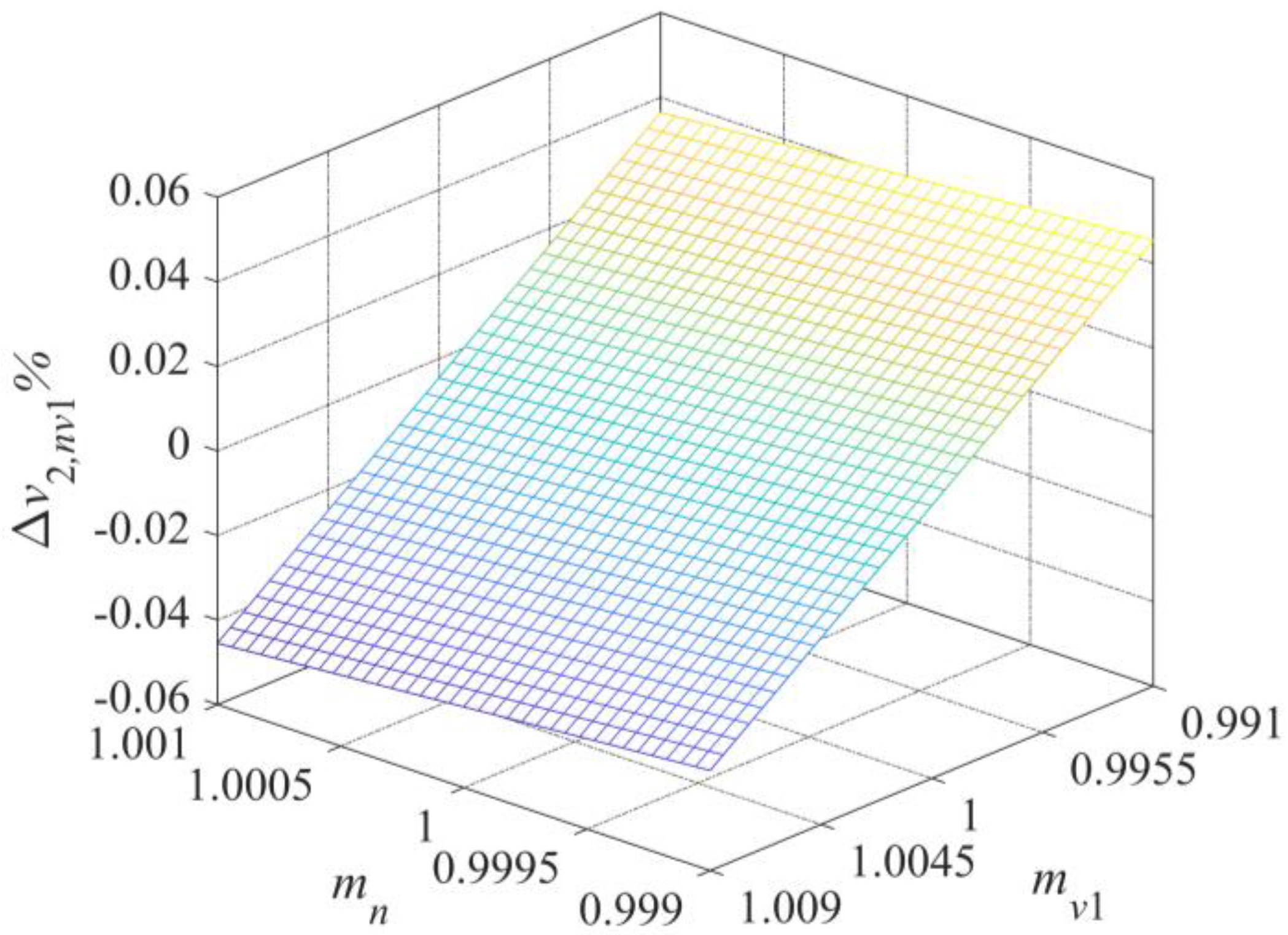
Figure 4 shows the percentage of steady-state error $\Delta v_{2,nv1}\%$ according to $m_n$ and $m_{v1}$. The range of mismatch ratios is shown in Table 3. According to LEM manufacture (current transducer LA 55-P and voltage transducer LV 25-P), the sensor accuracy is typically less than 0.9%. For the accuracy of $n$, it is easily measured by electronic equipment. Thus, it is clear that the mismatch of 0.1% is acceptable. From Figure 4, it is easy to see that $\Delta v_{2,nv1}\%$ has a maximum value of 0.0454% and a minimum value of −0.0455%. Obviously, these values are close to zero.

Similarly, the mismatch ratios of the output current $i_2$ and output voltage $v_2$ are defined as

$$\begin{array}{l}{m}_{i2}=\frac{i_{2act}}{i_2}\\ m_{v2}=\frac{v_{2act}}{v_2}\end{array}$$

(18)

where $i_{2act}$ and $v_{2act}$ are the actual values of $i_2$ and $v_2$, respectively.

Thus, the output voltage in the steady state is as follows

$$v_{2,i2v2}=\frac{fR{C}_2{m}_{i2}{m}_{v2}{v}_{2r}}{1-m_{i2}{m}_{v2}+fR{C}_2{m}_{i2}{m}_{v2}}.$$

(19)

From (19), the percentage of steady-state error $\Delta v_{2,i2v2}\%$ according to $m_{i2}$ and $m_{v2}$ is derived as follows

$$\Delta v_{2,i2v2}\%=\frac{v_{2,i2v2}-v_{2r}}{v_{2r}}\times 100\%=\frac{m_{i2}{m}_{v2}-1}{1-m_{i2}{m}_{v2}+fR{C}_2{m}_{i2}{m}_{v2}}\times 100\%.$$

(20)

Figure 5 shows the percentage of steady-state error $\Delta v_{2,i2v2}\%$ according to $m_{i2}$ and $m_{v2}$. The range of mismatch ratios is shown in Table 3. $\Delta v_{2,i2v2}\%$ has a maximum value of 0.0808% and a minimum value of −0.0829%. Similar to $\Delta v_{2,nv1}\%$, these values are close to zero.

Table 5. Comparison of the percentages of steady-state error.

Percentage of Steady-State Error	Minimum	Maximum
$\Delta v_{2,LC2}\%$	–1.4006%	0.9560%
$\Delta v_{2,nv1}\%$	–0.0455%	0.0454%
$\Delta v_{2,i2v2}\%$	–0.0829%	0.0808%

and Figure 6 compare all the percentages of steady-state error. It is clear that $\Delta v_{2,LC2}\%$ has the highest absolute value, while both $\Delta v_{2,nv1}\%$ and $\Delta v_{2,i2v2}\%$ have very small values. That means system parameters $L$ and $C_2$ have the most effect on the output voltage compared to the other parameters. Thus, the effects of the transformer turn ratio $n$ and the sensor accuracies ($v_1$, $v_2$, and $i_2$) can be considered trivial. Moreover, this effect can be overcome if a robust and adaptable controller is utilized. Fortunately, MDCS-MPC combined with the parameter identification technique is regarded as one of the advanced control methods with a high capacity of robustness and adaptiveness [1,2,3,4,5,6]. The effectiveness of the proposed controller will be presented in detail in Section 5.

From the analysis mentioned above, it is concluded that system parameters $L$ and $C_2$ primarily affect the output voltage compared to the others. To analyze the effect of system parameters $L$ and $C_2$, the sensitivity theory is studied on how the uncertainty of the system model affects the steady-state performance [45,46]. Many approaches to performing a sensitivity analysis of multiple parameters have been developed, including derivative-based methods [47], one-at-a-time sampling [48], and regression analysis [49]. In this paper, the partial derivative-based method [47] involves taking the partial derivative of the output $Y$ with respect to an input factor $X$, which is utilized to achieve the task. Thus, the sensitivity can be derived by the following general equation

$$S_X^Y=\frac{\frac{\mathsf{\partial }Y}{Y}}{\frac{\mathsf{\partial }X}{X}}=\frac{X}{Y}\frac{\mathsf{\partial }Y}{\mathsf{\partial }X}.$$

(21)

Therefore, the sensitivities $S_{m_L}^{v_2}$ and $S_{m_{C2}}^{v_2}$ of $L$ and $C_2$ to the output voltage $v_2$, respectively, are derived according to (13) and (21) as follows

$$S_{m_L}^{v_2}=\frac{m_L}{v_2}\frac{\mathsf{\partial }{v}_2}{\mathsf{\partial }{m}_L}=\frac{fR{C}_2{m}_L{m}_{C2}{v}_{2r}}{v_2{\left(1-m_L+fR{C}_2{m}_L{m}_{C2}\right)}^2}$$

(22)

$$S_{m_{C2}}^{v_2}=\frac{m_{C2}}{v_2}\frac{\mathsf{\partial }{v}_2}{\mathsf{\partial }{m}_{C2}}=\frac{fR{C}_2{m}_L{m}_{C2}{v}_{2r}\left(1-m_L\right)}{v_2{\left(1-m_L+fR{C}_2{m}_L{m}_{C2}\right)}^2}.$$

(23)

From (22) and (23), the values of $S_{m_L}^{v_2}$ and $S_{m_{C2}}^{v_2}$ are shown in Figure 7 with parameters in Table 4. Obviously, $S_{m_L}^{v_2}$ is a greater distance from 0 than $S_{m_{C2}}^{v_2}$, and as a result, the sensitivity of $L$ has a more significant impact on the system compared to $C_2$. $S_{m_{C2}}^{v_2}$ has minimum and maximum values at −0.0097 and 0.0138, respectively, while $S_{m_L}^{v_2}$ has minimum and maximum values at 0.0320 and 0.0690, respectively. Moreover, according to Figure 3, it is easy to see that when $L$ has a mismatch, $C_2$ also affects $\Delta v_{2,LC2}\%$. Therefore, $L$ and $C_2$ must be identified online together to improve the steady-state performance of the DAB converter.

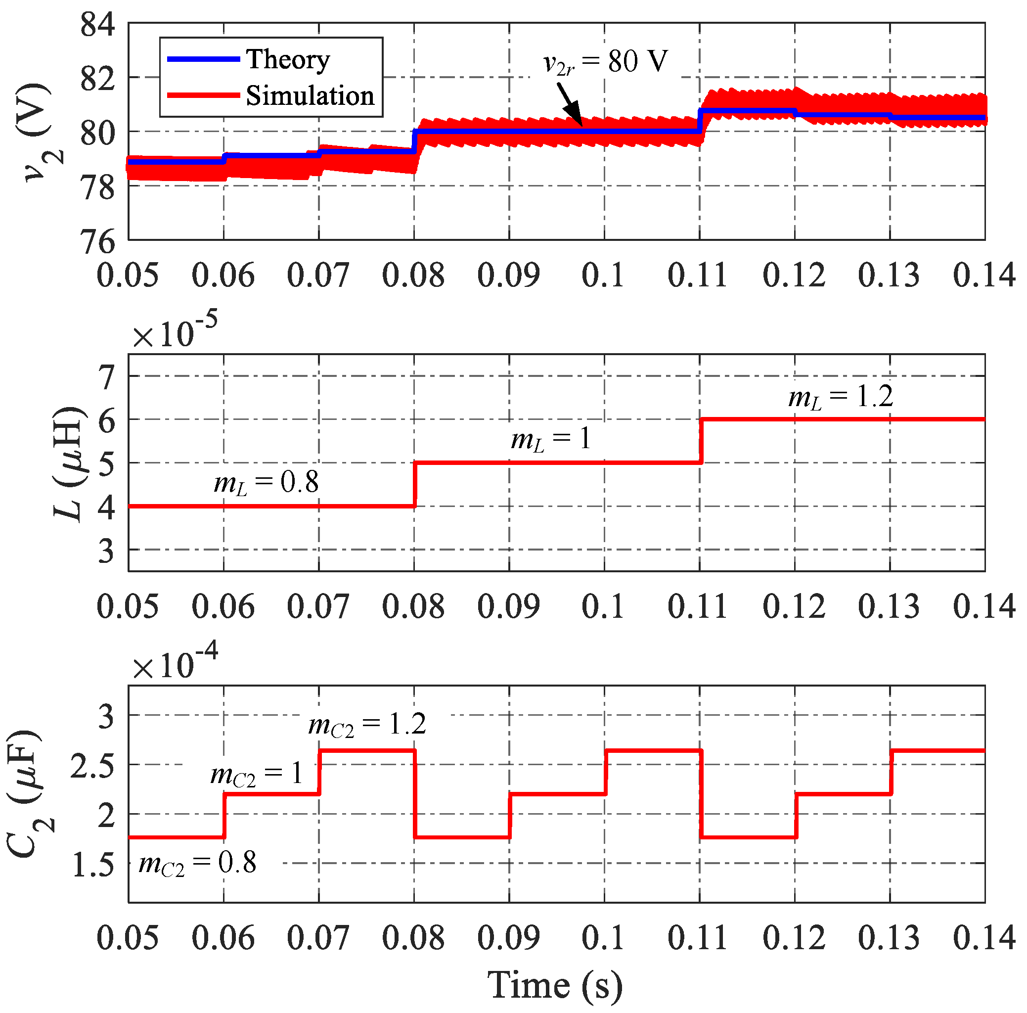
Figure 8 shows simulation results of MDCS-MPC with various mismatches of $L$ and $C_2$. System parameters are shown in Table 4, and the control variables of MDCS-MPC are shown in

Table 6. Controller parameters.

Meaning	Symbol	Value
Number of points	μ	11
Weighting factor	$c_1$	1
Weighting factor	$c_2$	5
Finest phase shift	${\Delta }_f$	1 × 10−5
Coefficient	$\lambda$	1
Saturated voltage	$V_m$	10 V

. Note that the number of points μ is chosen to balance performance and complexity. The output voltage is controlled at 80 V. Obviously, there is no steady-state error from 0.08 s to 0.11 s when $L$ and $C_2$ have actual values ($L$ = 50 μH and $C_2$ = 220 μF, meaning $m_L$ = $m_{C2}$ = 1). When $m_L$ = $m_{C2}$ = 0.8, the steady-state error has a minimum value, while it has a maximum value when $m_L$ = 1.2 and $m_{C2}$ = 0.8. In other instances of mismatch, there are also the steady-state errors. On the other hand, the simulation result is primarily consistent with the theoretical analysis, proving the effectiveness of theoretical analysis and the effect of $L$ and $C_2$ on MDCS-MPC in steady-state operation.

5. Parameter Identification Technique

As in the detailed analysis in Section 4, there are steady-state errors of $v_2$ in MDCS-MPC when the system parameters $L$ and $C_2$ have mismatch values. Thus, their parameters are identified online using a simple parameter identification technique, as presented below.

From (1)–(6), the constraint of the output voltage between sampling steps is derived as follows

$$v_2\left[k+2\right]=\frac{n{v}_1\left[k+1\right]}{2f^{2}L{C}_2}D\left[k+1\right]\left(1-D\left[k+1\right]\right)+\frac{n{v}_1\left[k\right]}{2f^{2}L{C}_2}D\left[k\right]\left(1-D\left[k\right]\right)-\frac{2}{f{C}_2}{i}_2\left[k\right]+v_2\left[k\right].$$

(24)

By rearranging (24), we obtain

$$\frac{n}{2f^2}\left(v_1\left[k+1\right]D\left[k+1\right]\left(1-D\left[k+1\right]\right)+v_1\left[k\right]D\left[k\right]\left(1-D\left[k\right]\right)\right)\frac{1}{L}+\left(v_2\left[k\right]-v_2\left[k+2\right]\right)C_2=\frac{2}{f}{i}_2\left[k\right].$$

(25)

From (25), the following is obtained

$$\alpha \left[k\right]\frac{1}{L}+u\left[k\right]C_2=\beta \left[k\right]$$

(26)

where

$$\alpha \left[k\right]=\frac{n}{2f^2}\left(v_1\left[k+1\right]D\left[k+1\right]\left(1-D\left[k+1\right]\right)+v_1\left[k\right]D\left[k\right]\left(1-D\left[k\right]\right)\right)$$

(27)

$$\beta \left[k\right]=\frac{2}{f}{i}_2\left[k\right]$$

(28)

$$u\left[k\right]=v_2\left[k\right]-v_2\left[k+2\right].$$

(29)

By rearranging (25) to the matrix form, the following is obtained

$$Ax=b$$

(30)

where $A\in {ℝ}^{k\times 2}$, $x\in {ℝ}^2$, and $b\in {ℝ}^{k\times 1}$, presented as follows

$$A=\left[\begin{array}{cc}\begin{array}{c}\alpha \left[k\right]\\ \epsilon \alpha \left[k-1\right]\\ ⋮\\ {\epsilon }^{k-1}\alpha \left[1\right]\end{array}& \begin{array}{c}u\left[k\right]\\ \epsilon u\left[k-1\right]\\ ⋮\\ {\epsilon }^{k-1}u\left[1\right]\end{array}\end{array}\right]$$

(31)

$$x={\left[\begin{array}{cc}\frac{1}{L}& C_2\end{array}\right]}^T$$

(32)

$$b={\left[\begin{array}{cccc}\beta \left[k\right]& \epsilon \beta \left[k-1\right]& \dots & {\epsilon }^{k-1}\beta \left[1\right]\end{array}\right]}^T.$$

(33)

In (31)–(33), constant $\epsilon$ is the forgetting factor. Considering that the abrupt alteration in operating scenarios (for instance, reference voltage steps up, etc.) and the system parameters (for instance, one of the parallel capacitors is damaged, etc.) renders the previously measured data less critical, and the impacts of such data must rapidly disappear. When $v_2$ is somewhat near $v_{2r}$, the previously measured data should be required less frequently as the sampling step increases. In most cases, the range 0 < ε < 1 is selected for the variable to provide versatility. If $\epsilon$ is too small (close to zero), the estimator’s performance will suffer since it will be more susceptible to being affected by noise or disturbance. On the contrary, when $\epsilon$ approaches 1, there is a slight forgetting effect. This means that the solution of the proposed approach is mainly driven by the previously obtained data, which slows down the convergence speed. In regular hardware operation, $L$ and $C_2$ are usually subject to slow variation, resulting in $\epsilon$ needing to be set as close as possible to 1. In this paper, $\epsilon$ = 0.99 is used.

From (30)–(33), the following expression is obtained

$$e=Ax-b.$$

(34)

By using the LSA according to [36], a mean square error is derived as follows

$$L\left(x\right)={‖e‖}^2={\left(Ax-b\right)}^T\left(Ax-b\right).$$

(35)

In order to obtain a unique minimizer, a derivation is as follows

$$\frac{\mathsf{\partial }L\left(x\right)}{\mathsf{\partial }x}=2A^{T}Ax-2A^{T}b=0.$$

(36)

As a result, $x$ is obtained as follows

$$x={\left(A^{T}A\right)}^{-1}{A}^{T}b.$$

(37)

The online identification of $x$ is accomplished by substituting (31)–(33) into (37). On the other hand, the matrix and vector both have a growing number of rows, which significantly burdens the controller and makes the solution impracticable. Therefore, (38) should be rewritten to reduce the dimensionality of all the matrices and vectors

$$x={\left(\Omega \right)}^{-1}\phi$$

(38)

where

$$\Omega =\left[\begin{array}{cc}{\omega }_{11}\left[k-1\right]& {\omega }_{12}\left[k-1\right]\\ {\omega }_{21}\left[k-1\right]& {\omega }_{22}\left[k-1\right]\end{array}\right]=A^{T}A$$

(39)

$$\phi =\left[\begin{array}{c}{\phi }_1\left[k-1\right]\\ {\phi }_2\left[k-1\right]\end{array}\right]=A^{T}b.$$

(40)

Therefore, the elements from (39) and (40) can be calculated as follows

$$\begin{array}{l}{\omega }_{11}\left[k-1\right]={\displaystyle \sum _{h=1}^{k-1}{\left({\epsilon }^{k-1-h}\alpha \left[h\right]\right)}^2}\\ {\omega }_{12}\left[k-1\right]={\omega }_{21}\left[k-1\right]={\displaystyle \sum _{h=1}^{k-1}{\left({\epsilon }^{k-1-h}\right)}^2\alpha \left[h\right]u\left[k\right]}\\ {\omega }_{22}\left[k-1\right]={\displaystyle \sum _{h=1}^{k-1}{\left({\epsilon }^{k-1-h}u\left[k\right]\right)}^2}\\ {\phi }_1\left[k-1\right]={\displaystyle \sum _{h=1}^{k-1}{\left({\epsilon }^{k-1-h}\right)}^2\alpha \left[h\right]}\beta \left[h\right]\\ {\phi }_2\left[k-1\right]={\displaystyle \sum _{h=1}^{k-1}{\left({\epsilon }^{k-1-h}\right)}^2\beta \left[h\right]u\left[k\right]}.\end{array}$$

(41)

From the point of view of (41), there is a successive recurrence relation of the elements in order to ensure the easy implementation of the proposed approach, as shown in (42)

$$\begin{array}{l}{\omega }_{11}\left[k-1\right]={\alpha }^2\left[k-1\right]+{\epsilon }^2{\omega }_{11}\left[k-2\right]\\ {\omega }_{12}\left[k-1\right]={\omega }_{21}\left[k-1\right]=\alpha \left[k-1\right]u\left[k\right]+{\epsilon }^2{\omega }_{12}\left[k-2\right]\\ {\omega }_{22}\left[k-1\right]=u^2\left[k\right]+{\epsilon }^2{\omega }_{22}\left[k-2\right]\\ {\phi }_1\left[k-1\right]=\alpha \left[k-1\right]\beta \left[k-1\right]+{\epsilon }^2{\phi }_1\left[k-2\right]\\ {\phi }_2\left[k-1\right]=\beta \left[k-1\right]u\left[k\right]+{\epsilon }^2{\phi }_2\left[k-2\right].\end{array}$$

(42)

Different from the matrix $A$ and vector $b$ having many elements, $\Omega \in {ℝ}^{2\times 2}$ and $\phi \in {ℝ}^2$. Thus, a simple calculation of the inverse matrix ${\Omega }^{-1}$ significantly mitigates the calculation burden.

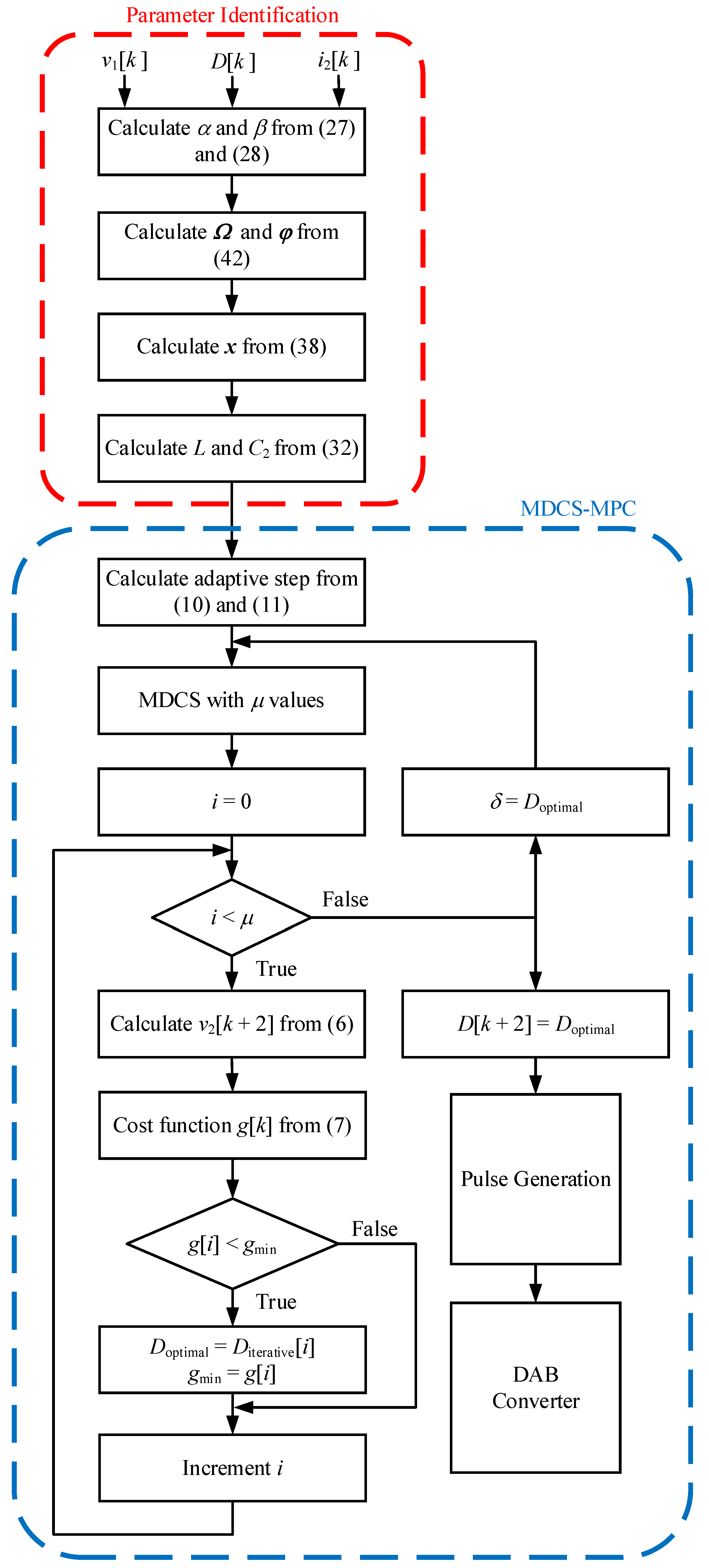
The flowchart of the proposed method is shown in Figure 9. First, $\alpha$ and $\beta$ are derived from (27) and (28), respectively. Then, $\Omega$ and $\phi$ are calculated from (42), while x is calculated from (38). After the system parameters $L$ and $C_2$ are identified online from (32), the adaptive step of MDCS-MPC is calculated based on (10) and (11). MDCS-MPC will generate a range of phase-shift ratios with the number of points μ. Then, the iteration starts for MDCS-MPC by comparing values of the cost function of corresponding phase-shift ratios to find the optimal values of $D$.

6. Simulation Verification

In this section, the effectiveness of the proposed method is verified through simulation. In addition, the dynamic performance of MDCS-MPC is compared with PI control under match system parameters. Gains of PI control are designed according to [50].

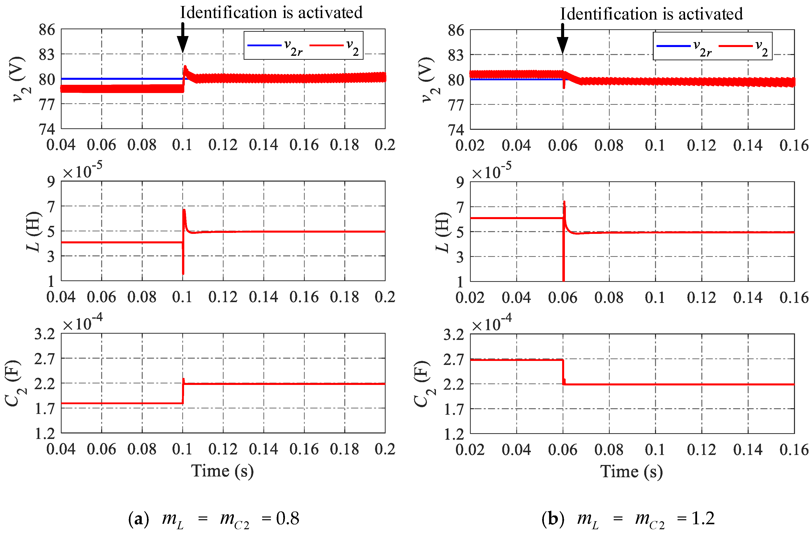
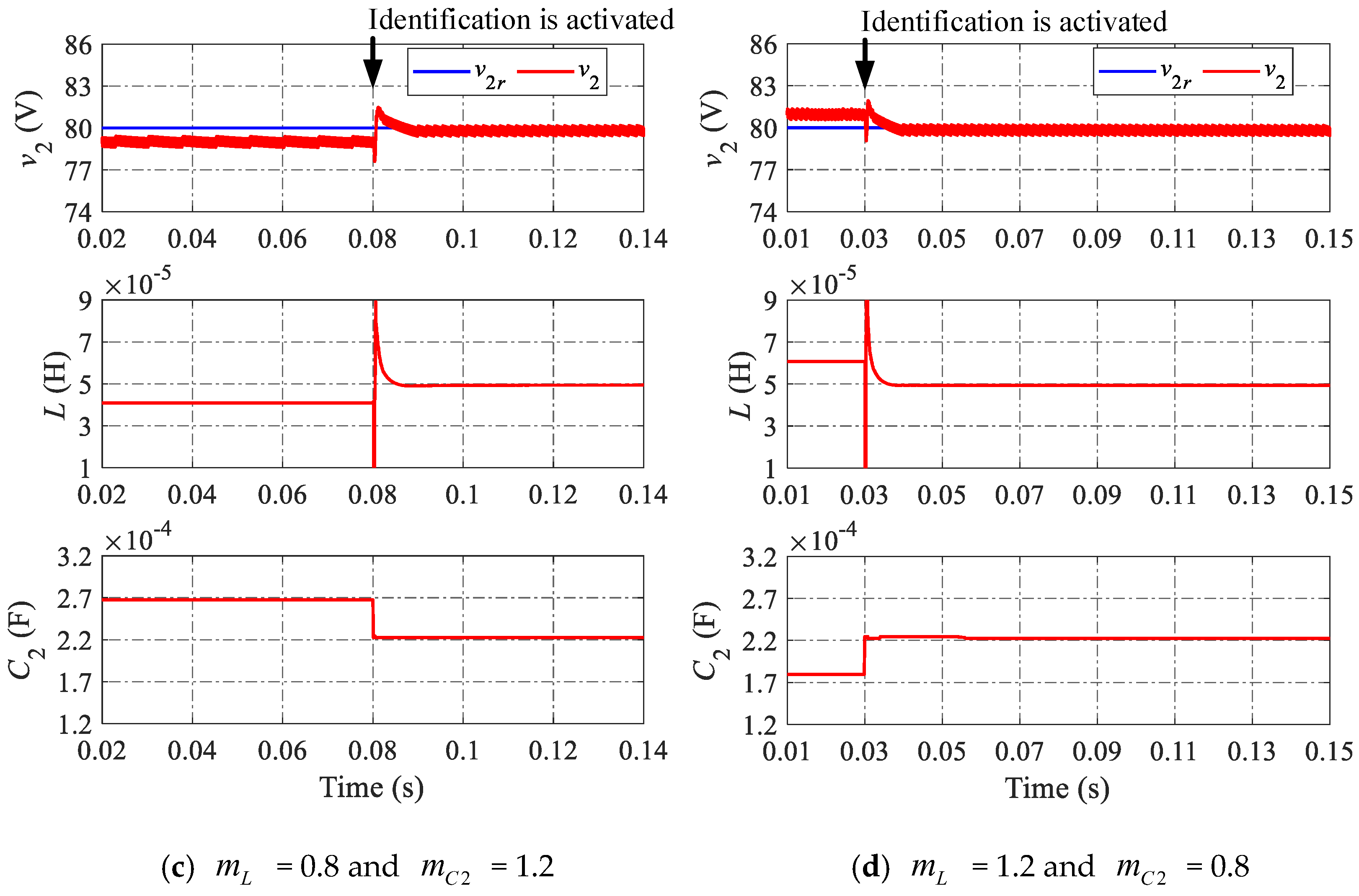
Figure 10 shows the steady-state error of $v_2$ in MDCS-MPC before and after parameter identification. Initially, MDCS-MPC operates under mismatch parameters, as shown in Figure 10a, showing the steady-state error from 0.04 s to 0.1 s. However, when the parameter identification technique is applied at 0.1 s, the steady-state error immediately disappears, meaning the steady-state performance is immediately improved. Moreover, the values of $L$ and $C_2$ are also identified online as the actual values. Obviously, when MDCS-MPC is combined with the parameter identification technique, the steady-state performance of the proposed controller is significantly improved. Similar to Figure 10a, other cases of mismatch system parameters are shown in Figure 10b–d. When the parameter identification technique is applied, the steady-state error immediately disappears. It is easy to conclude that both steady-state and identification performances also prove the effectiveness of the proposed method.

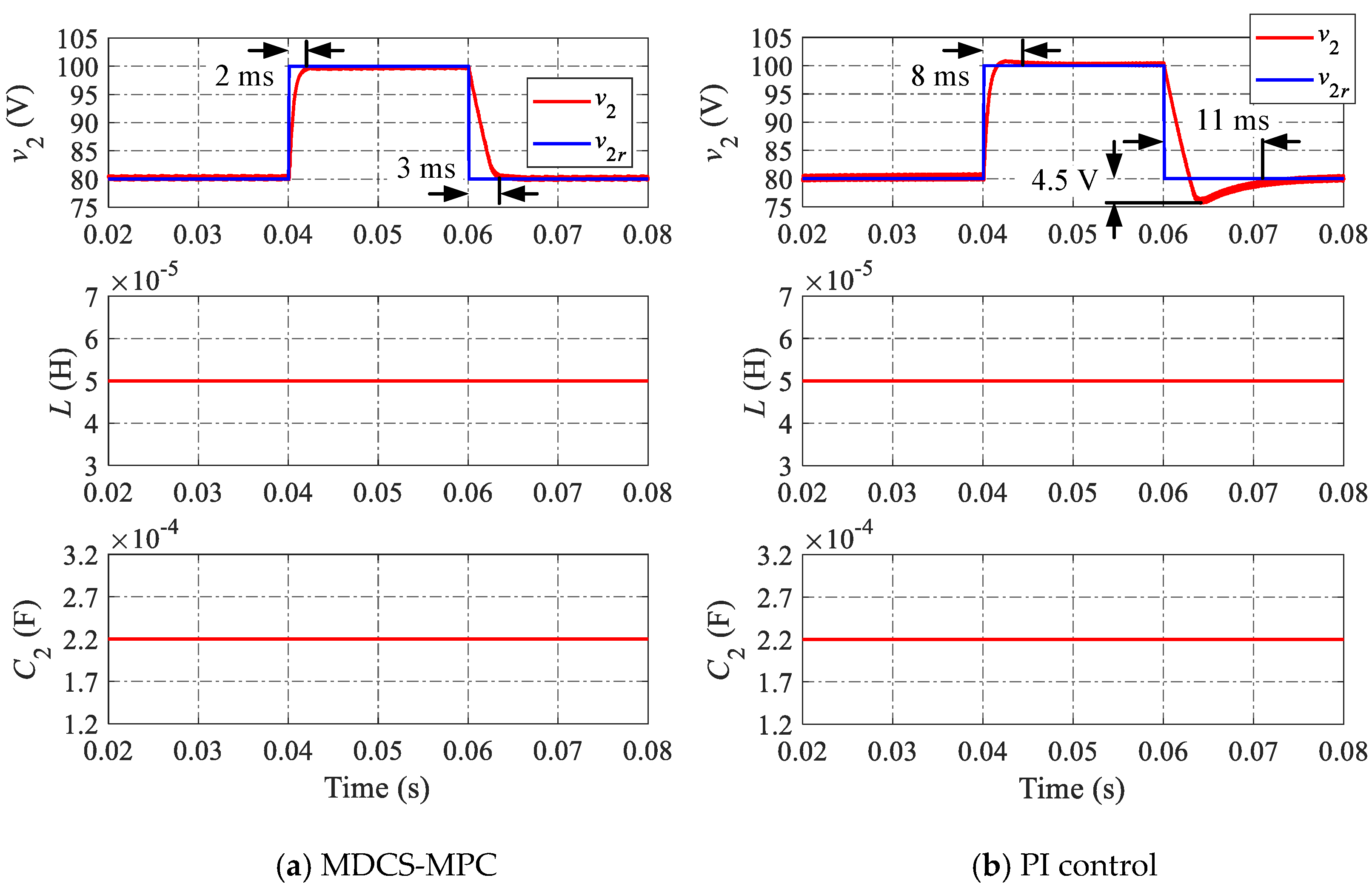
As shown in Figure 11, MDCS-MPC is compared with the PI control under the match system parameters. When $v_{2r}$ steps up at 0.04 s, the MDCS-MPC costs 2 ms for settling time with overshoot-free, while the PI control costs 8 ms with a slight overshoot value. On the other hand, when $v_{2r}$ steps down at 0.06 s, the MDCS-MPC costs 3 ms for settling time with undershoot-free, while the PI control costs 11 ms with an undershoot of 4.5 V. Obviously, compared to the PI control, the MDCS-MPC provides better dynamic performance for the reference voltage change step.

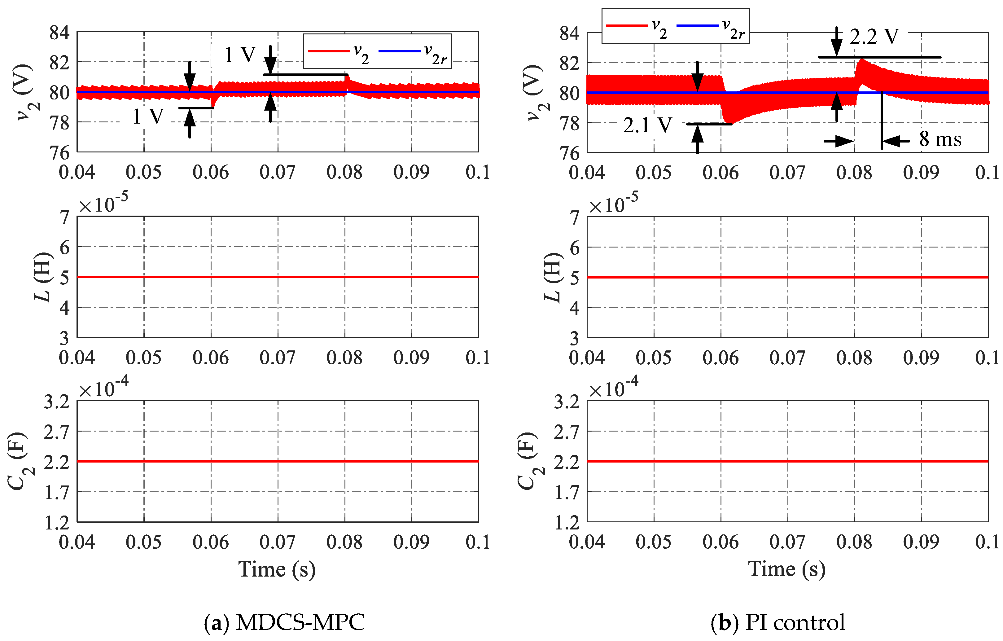
Figure 12 compares the dynamic performance of the output voltage of the two methods under the match system parameters. When $i_2$ steps up at 0.06 s, the MDCS-MPC shows 1 V for undershoot, while the PI control shows 2.1 V. On the other hand, when $i_2$ steps down at 0.08 s, the MDCS-MPC shows 1 V for overshoot, while the PI control shows 2.2 V for overshoot with 8 ms for settling time. Obviously, compared to the PI control, the MDCS-MPC also provides better dynamic performance when changing the output current.

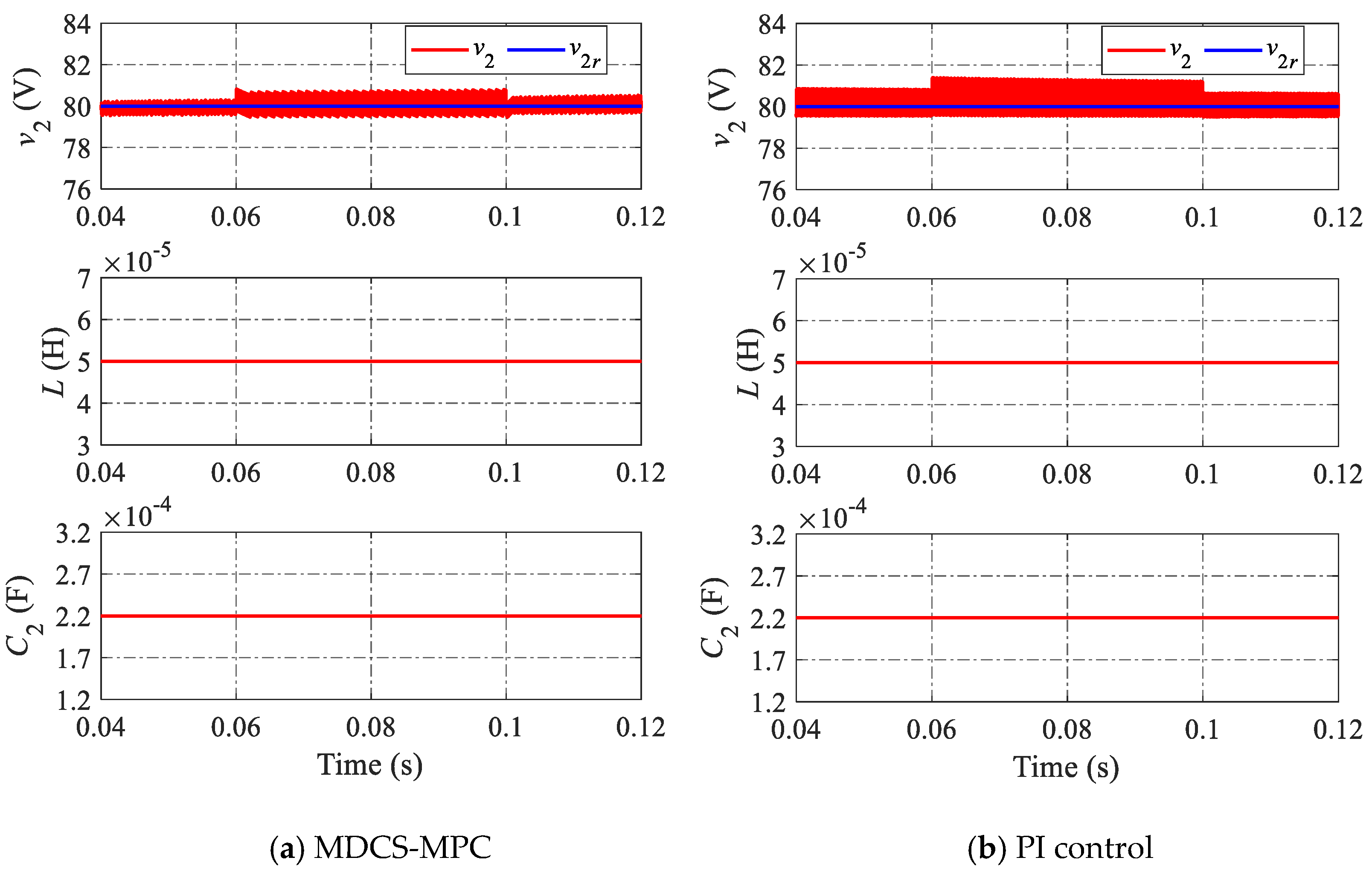
Figure 13 shows the simulation results when the input voltage $v_1$ steps up from 95 V to 100 V at 0.06 s and steps down from 100 V to 95 V at 0.1 s under the match system parameters. When $v_1$ changes, both MDCS-MPC and PI control have good dynamic performance, but there are more voltage ripples in the PI control compared to the MDCS-MPC.

7. Conclusions

This paper proposed a combination of MDCS-MPC and the online parameter identification technique for controlling the DAB converter, aiming to improve the steady-state performance of the output voltage. The contributions are briefly summarized as follows:

• Key model parameters for the DAB converter are found by analysis of the percentage of steady-state error of the output voltage, and sensitivity analysis of the system parameters is derived mathematically;
• LSA is used to identify online system parameter values, resulting in improved steady-state performance.

Furthermore, the dynamic performance of MDCS-MPC reveals that it is superior to PI control. Simulation verification was carried out to demonstrate the robustness of the proposed method in terms of parameter variation.