Modeling Asymmetric Dependence Structure of Air Pollution Characteristics: A Vine Copula Approach

Abstract

Contaminated air is unhealthy for people to breathe and live in. To maintain the sustainability of clean air, air pollution must be analyzed and controlled, especially after unhealthy events. To do so, the characteristics of unhealthy events, namely intensity, duration, and severity are studied using multivariate modeling. In this study, the vine copula approach is selected to study the characteristics data. Vine copula is chosen here because it is more potent than the standard multivariate distributions, and multivariate copulas, especially in modeling the tails related to extreme events. Here, all nine different vine copulas are analyzed and compared based on model fitting and the comparison of models. In model fitting, the best model obtained is Rv123-Joint-MLE, a model with a root nodes sequence of 123, and optimized using the joint maximum likelihood. The components for the best model are the Tawn type 1 and Rotated Tawn type 1 180 degrees representing the pair copulas of (intensity, duration), and (intensity, severity), respectively, with the Survival Gumbel for the conditional pair copula of (duration, severity; intensity). Based on the best model, the tri-variate dependence structure of the intensity, duration, and severity relationship is positively correlated, skewed, and follows an asymmetric distribution. This indicates that the characteristic’s, including intensity, duration, and severity, tend to increase together. Using comparison tests, the best model is significantly different from others, whereas only two models are quite similar. This shows that the best model is well-fitted, compared to most models. Overall, this paper highlights the capability of vine copula in modeling the asymmetric dependence structure of air pollution characteristics, where the obtained model has a better potential to become a tool to assess the risks of extreme events in future work.

1. Introduction

Maintaining clean air is an important task to sustain the health of people and nature. However, human activities such as urbanization, transportation, industrialization, open burning, and forest fires contribute to degrade air quality [1]. Many serious diseases such as obstructive pulmonary diseases, lung cancer, and cardiovascular diseases are associated with air pollution [2,3,4,5]. People with severe heart and lung complications tend to suffer at most when exposed to air pollutants, especially fine particles [6]. A recent survey showed that air pollutants can also aggravate psychological dilemmas, trigger financial downturns, and create social issues [7]. These highlight the importance of monitoring and managing the risks of unhealthy air pollution emergencies. 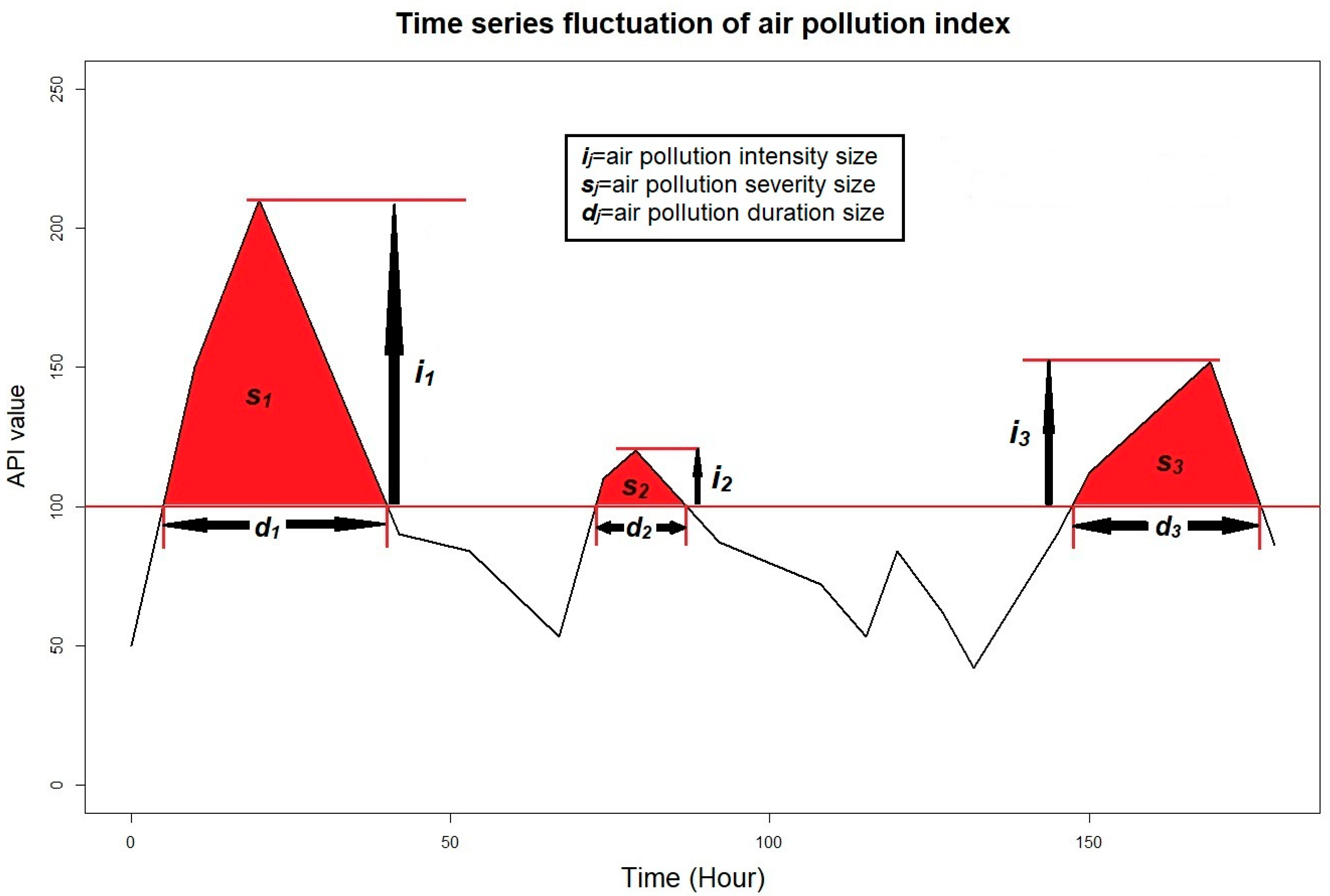For monitoring, the composite index of pollutants (carbon monoxide CO, ozone O₃, nitrogen dioxide NO₂, sulfur dioxide SO₂, and fine particles with a size less than 10 microns PM₁₀) is used and is usually called an air pollution index (API) [8,9]. In Malaysia, API values exceeding 100 within certain periods are considered unhealthy events. Such events are also associated with haze [10]. Therefore, above the 100 level, if the API value keeps increasing, air pollution will become more intense.

In assessing air pollution in Peninsular Malaysia, the Pareto distribution has been used to investigate API data from eight main cities with Klang being identified as the most exposed city [11]. The lognormal, exponential, Gamma, and Weibull distributions were also examined to model the API data and its sub-indexes in Kuala Lumpur, and it was reported that the Gamma distribution is the best distribution for most data [12]. Sub-indexes of API during unhealthy events were also investigated using the generalized Pareto distribution to conclude that PM₁₀ and O₃ are the most severe pollutants [13]. Besides local sources, the concentration of PM₁₀ and O₃ are also related to regional tropical factors, such as the influence of biomass burning and ultraviolet radiation from sunlight [14]. Based on this, the call for reducing PM₁₀ volume is emphasized since it is the main contributor to unhealthy air pollution in Klang [15,16]. In [17], gaseous pollutants, particularly O₃, are also urged to be reduced since gaseous pollutants are more harmful to respiratory and natural mortalities compared to particles.

It was also reported that a significant reduction in the concentration of air pollutants (PM₁₀, PM_2.5, NO₂, and CO) occurred during the COVID-19 movement control order in Malaysia, and this reduction is believed to be due to a decrease in the use of vehicles on the roads [18]. In [19], three different methods, called conventional models, API structure models, and descriptive status models, were applied to analyze the API data and showed that these methods have their individual advantages and that the mixture approach is a better way to simulate the API data. The mixed approach is better because the conventional fitted models are capable of distinguishing API status (healthy or unhealthy), the API structure models are superior to modeling the API data, and the API descriptive status models are useful to determine the return level for unhealthy events.

In addition, the stochastic dependence of API data in Klang was also investigated using a discrete-time Markov chain model and concluded that the occurrence of unhealthy events is relatively small, but that these events are quite troubling [20]. In [21], the Hierarchical-Generalized Pareto model is applied to API data from different locations to provide a precise estimation of the return levels for each location. Moreover, the mixed peak-over-threshold-block-maxima (POT-BM) approach was used to investigate the unhealthy events and showed that this approach has an excellent tradeoff between bias and variance in modeling the extreme events [22].

Furthermore, flexible multivariate modeling via the copula approach was also used to examine the dynamic dependence structure between PM₁₀ and other air pollutants [23]. Using a multifractal technique on API in Klang, Masseran [24] showed that hourly API data contains the most information on air pollution and that the data reduction process is affected by the data duration. Moreover, survey data obtained from the cross-sectional survey is used to study Malaysians’ awareness of air pollution and its related impacts on human health, where the surveys pointed out the need to increase the awareness of air pollution among Malaysian [25,26]. A recent survey on air pollution and its health impacts in Malaysia is also discussed in [27]. Based on the monthly air pollution hospitalization dataset in Klang Valley, Malaysia, artificial intelligence techniques are also used to predict the trends of cardiorespiratory hospitalization due to air pollution [28].

Besides API, air pollutants time series, survey data, and air pollution hospitalization dataset, characteristics of unhealthy events such as severity, intensity, and duration are also explored to understand the behaviors of air pollution. For instance, the intensity–duration–frequency approach has been applied to describe the relationship between intensity with duration and also return period, where findings warned that intensity in Klang moves in the same direction as duration and return period [29,30]. Focusing on modeling the duration distribution, the Lognormal distribution is showed to provide a better fit than Exponential, Gamma, and Weibull distributions [31]. Furthermore, by using the power-law model, prolonged air pollution with a duration of more than 33 h is believed to be the threshold for events with power-law behaviors, indicating the risks of unhealthy events [32]. In addition, the generalized extreme-value (GEV) model has also been used to study severity data and found that the severity in Klang tends to increase together with the length of return periods [33].

On the other hand, the dependence relationship between severity and duration in Klang was also analyzed using bivariate copula models for planning and risk mitigation purposes [34]. As a continuation of [34], an additional study has been done to include intensity in the analysis together with severity and duration, then various bivariate copula models were applied to examine the bivariate dependence structures for three pairs, which are (duration, intensity), (severity, intensity), and (duration, severity) [35]. The latter showed that the dependence structures for the pairs were skewed and asymmetric. However, the tri-variate relationship of the duration–intensity–severity is yet to be explored. In this study, we analyze the tri-variate dependence structure of the intensity, duration, and severity using a vine copula approach. Vine copula is proposed here because it provides a more reliable, realistic, flexible, and tractable model compared to the standard multivariate distributions, and multivariate copulas, especially in modeling the tail behaviors related to extremely unhealthy events [36,37,38]. Therefore, this analysis can provide a new perspective to the existing information on air pollution data through the relationship between intensity, duration, and severity.

This paper is organized as follows: Section 2 introduces the vine copula approach, Section 3 describes the sample data, Section 4 discusses the proposed method, Section 5 provides results and discussions, and finally, Section 6 concludes this paper and provides a suggestion for future work.

2. Vine Copula

Vine copula is an enhanced copula approach, where the bivariate copulas and bivariate conditional copulas are used as building blocks to obtain a more flexible and tractable multivariate model for a joint distribution [36,37,38]. Furthermore, vine copula is more potent than the standard multivariate distributions and multivariate copulas, especially in modeling the asymmetric distributions and the tail behaviors related to extreme events [36,39,40].

In multivariate modeling, Sklar’s theorem stated that a joint distribution $F$ is equal to a copula distribution $C$, such that

$$F\left(x_1,x_2,\cdots ,x_d\right)=C\left(F_1\left(x_1\right),F_2\left(x_2\right),\cdots ,F_d\left(x_d\right)\right),$$

(1)

where $x_1,x_2,\cdots ,x_d$ are random variables and $F_1,F_2,\cdots ,F_d$ are marginal distributions [41,42]. For simplicity, $F_1\left(x_1\right),F_2\left(x_2\right),\cdots ,F_d\left(x_d\right)$ are also denoted by $u_1,u_2,\cdots ,u_d$ and called as copula variables. Since the random variables $U_{\mathrm{i}}=F_{\mathrm{i}}\left(X_i\right)$, $i=1,2,\cdots ,d$, are uniformly distributed on the closed unit interval $\left[\mathrm{0,1}\right]$, then a copula distribution $C\left(u_1,u_2,\cdots ,u_d\right)$ is a multivariate distribution function on the $d$-dimensional hypercube ${\left[0,1\right]}^d$.

The joint distribution $F$ in Equation (1) is absolutely continuous if the copula $C$ is absolutely continuous; that is, $C$ has a density function and the marginal distributions $F_1,\cdots ,F_d$ are continuous [36]. For this case, the obtained copula distribution $C$ is unique and the corresponding copula density $c$ can be obtained using partial derivative as follows

$$c\left(u_1,u_2,\cdots ,u_d\right)=\frac{{\partial }^d}{\partial u_1\partial u_2\cdots \partial u_d}C\left(u_1,u_2,\cdots ,u_d\right).$$

(2)

In the literature, there are many copula distributions that have been developed, especially for the bivariate copula $C\left(u_1,u_2\right)$ [43]. Some examples are Clayton, Franks, and Joe copulas. Functions for these copulas can be defined, respectively, as follows

$$C\left(u_1,u_2;\theta \right)={\left(u_1^{-\theta }+u_2^{-\theta }-1\right)}^{-\frac{1}{\theta }},$$

(3)

$$C\left(u_1,u_2;\theta \right)=-\frac{1}{\theta }\mathrm{l}\mathrm{n}\left[1+\frac{\left(e^{-\theta u_1}-1\right)\left(e^{-\theta u_2}-1\right)}{e^{-\theta }-1}\right]$$

(4)

$$C\left(u_1,u_2;\theta \right)=1-{\left[{\left(1-u_1\right)}^{\theta }+{\left(1-u_2\right)}^{\theta }-{\left(1-u_1\right)}^{\theta }{\left(1-u_2\right)}^{\theta }\right]}^{\frac{1}{\theta }},$$

(5)

where $\theta$ is an independent variable to the copulas [38,44].

From a bivariate distribution copula $C\left(u_1,u_2\right)$, some important dependence measures, including Kendall’s $\tau$ correlation, upper tail dependence ${\lambda }^{\mathrm{upper}}$, and lower tail dependence ${\lambda }^{\mathrm{lower}}$ coefficients also can be obtained. Kendall’s $\tau$ correlation coefficient measures the central dependency, upper tail dependence ${\lambda }^{\mathrm{upper}}$ coefficient computes the probability of the joint occurrence of extremely large values, and lower tail dependence ${\lambda }^{\mathrm{lower}}$ coefficient calculates the probability of the joint occurrence of extremely small values [36]. In addition, these coefficients can describe whether a bivariate copula has a skewed and asymmetric distribution. The formulas for these three coefficients can be obtained, respectively, as

$$\tau =4\underset{0}{\overset{1}{\int }}\underset{0}{\overset{1}{\int }}C\left(u_1,u_2\right)dC\left(u_1,u_2\right)-1,$$

(6)

$${\lambda }^{\mathrm{upper}}=\underset{t\to 1^{-}}{\lim }\frac{1-2t+C\left(t,t\right)}{1-t},$$

(7)

and

$${\lambda }^{\mathrm{lower}}=\underset{t\to 0^{+}}{\lim }\frac{C\left(t,t\right)}{t}.$$

(8)

In the vine copula approach, bivariate copulas are also known as pair copulas. By using the pair copula decompositions and constructions proses, a $d$-dimensional copula density $c$ can be transformed into a vine copula, as a product of $d\left(d-1\right)/2$ components, including pair and conditional pair copulas [45]. However, the obtained vine copula is not unique. For example, in the case of $d=3$, there are 3 vine copulas that exist with different compositions. By using a representation from the graph theory called a tree (an undirected, connected and acyclic graph), a vine copula can be illustrated as a trees sequence (also called a vine trees sequence) [46].

A vine trees sequence $\mathsf{\Sigma }=\left(T_1,\cdots ,T_{d-1}\right)$ on $d$ data is a sequence of trees $T_m=\left(N_m, E_m\right)$, $m=1,2,\cdots ,d-1$, if

• Each tree $T_m=\left(N_m, E_m\right)$ is a connected, i.e., for all nodes $a,b\in N_m$, $m=1,2,\cdots ,d-1$, there exits a path $n_1, n_2, \cdots , n_k\subset N_m$ with $a=n_1, b=n_k$.
• $T_1$ is a tree with node set $N_1=\left\{1, 2,\cdots ,d\right\}$ and edge set $E_1$.
• For $m\ge 2$, $T_m$ is a tree with node set $N_m=E_{m-1}$ and edge set $E_m$.
• (Proximity condition) Whenever two nodes in $T_{m+1}$ are joined by an edge, the corresponding edges in $T_m$ must share a common node, i.e., for $m=2, 3, \cdots , d-1$ and $\left\{a,b\right\}\in E_m$ it must hold that $\left|a\cap b\right|=1$ [38].

In a vine trees sequence, each edge $e$ can be denoted by $\left(j_e,k_e\right)$ for $T_1$ and $\left(j_e,k_e;D_e\right)$ for $T_m$, where $m=2, 3, \cdots , d-1$. The difference between those two notations is an edge for $T_m$, where $m=2, 3, \cdots , d-1$ is determined by two shared edges in the previous tree $T_{m-1}$. For $m=2, 3, \cdots , d-1$, let there is one node that shared two edges in the previous tree $T_{m-1}$ are denoted as $a=\left(j_a,k_a;D_a\right)$ and $b=\left(j_b,k_b;D_b\right)$ and the corresponding sets containing all indices of the two shared edges are denoted as ${\mathcal{V}}_a=\left\{j_a,k_a,D_a\right\}$ and ${\mathcal{V}}_b=\left\{j_b,k_b,D_b\right\}$, respectively. Then, in the next tree $T_m$, those the two shared edges become two nodes a and b, which connected by a new edge $e=\left(j_e,k_e;D_e\right)$, where $j_e=\min \left\{l:l\in \left({\mathcal{V}}_a\cup {\mathcal{V}}_b\right)\backslash D_e\right\}$ and $k_e=\max \left\{l:l\in \left({\mathcal{V}}_a\cup {\mathcal{V}}_b\right)\backslash D_e\right\}$ and $D_e={\mathcal{V}}_a\cap {\mathcal{V}}_b$. Here, $D_e$ and $\left\{j_e,k_e\right\}$ are sets of indices, which are called the conditioning and conditioned sets of the new edge $e$, respectively [38].

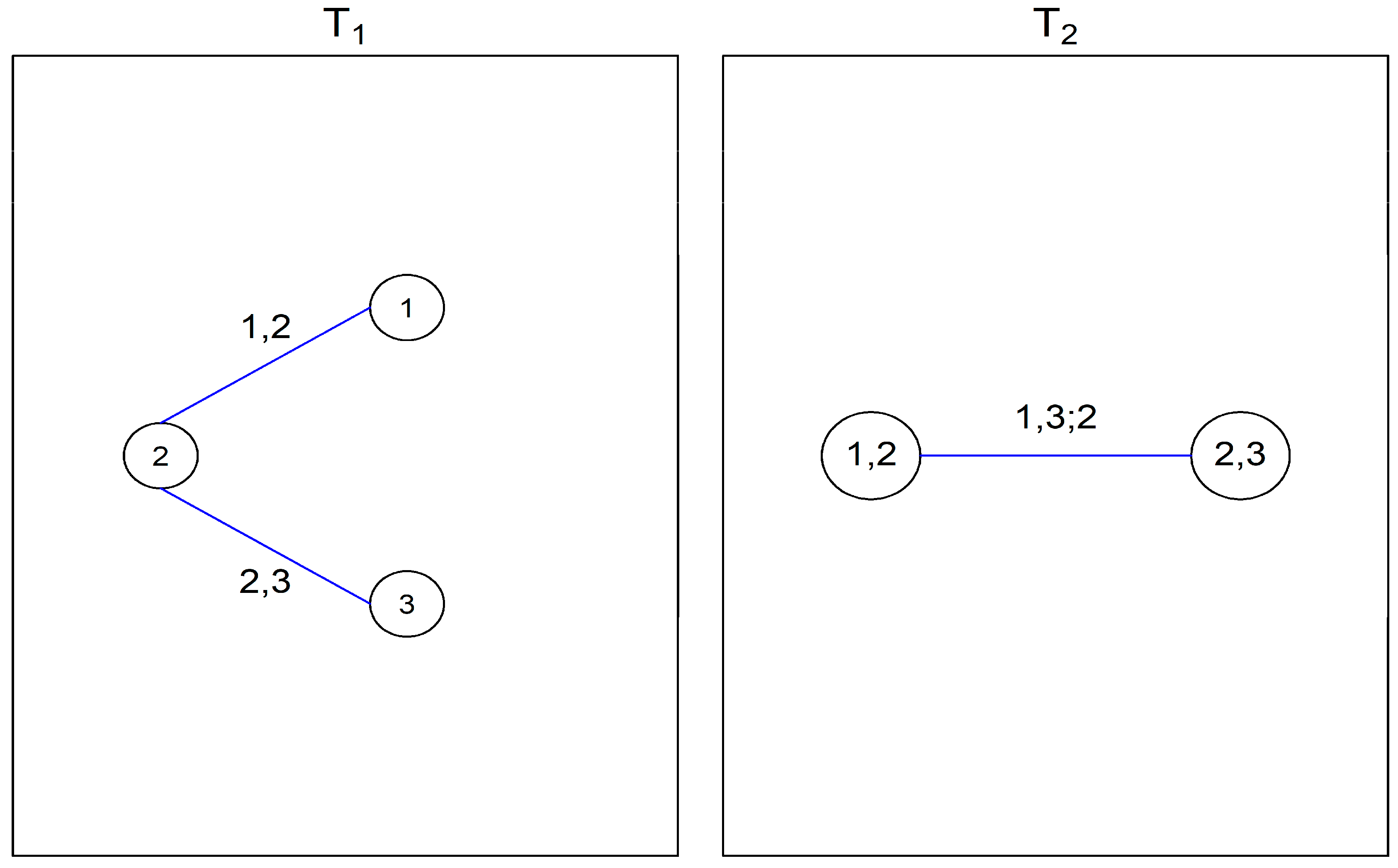
For example, in Figure 1, in the $T_1$, has a node (denoted by the index $2$) that shared two edges $a=\left(1,2\right)$ and $b=\left(2,3\right)$, with ${\mathcal{V}}_a=\left\{1,2\right\}$ and ${\mathcal{V}}_b=\left\{2,3\right\}$. Then, in the $T_1$, those two shared edges become two nodes a and b, and they are connected by a new edge $e=\left(1,3;2\right),$ where $j_e=1$ and $k_e=3$ and $D_e=\left\{2\right\}$. In this case, $\left\{2\right\}$ and $\left\{1,3\right\}$ are the conditioning and conditioned sets of the new edge $e=\left(1,3;2\right),$ respectively.

Generally, a vine copula (also known as a regular vine copula) is a multivariate modeling made up of a combination of pair copulas and pair conditional copulas to model the dependence structure of $d-$dimensional copula data $\mathit{U}=\left(U_1,U_2,\cdots ,U_d\right)$ and its components can be visualized using a vine trees sequence.

For a regular vine copula, its general density can be written as

$$c\left(\mathit{u}\right)=\prod _{m=1}^{d-1}\prod _{e\in E_m}{c}_{j_e,k_e;D_e}\left(C_{j_e|D_e}\left(u_{j_e}|{\mathit{u}}_{D_e}\right),C_{k_e|D_e}\left(u_{k_e}|{\mathit{u}}_{D_e}\right);{\mathit{u}}_{D_e}\right),$$

(9)

where ${\mathit{u}}_{D_e}={\left(u_{\mathit{l}}\right)}_{\mathit{l}\in D_e}$ is a subvector of $\mathit{u}=\left(u_1,u_2,\cdots ,u_{\mathit{d}}\right)\in {\left[\mathrm{0,1}\right]}^{\mathit{d}}$, $C_{j_e|D_e}$ is the conditional distribution of $U_{j_e}|{\mathit{U}}_{D_e}={\mathit{u}}_{D_e}$, and $c_{j_e,k_e;D_e}$ is the copula density corresponding to the two variables $C_{j_e|D_e}$ and $C_{k_e|D_e}$, conditional on ${\mathit{U}}_{D_e}={\mathit{u}}_{D_e}$.

In Equation (9), each pair copula density $c_{j_e,k_e;D_e}$ depends on the conditioning vector ${\mathit{u}}_{D_e}$. In practice, to reduce the complexity, a simplifying assumption is made, which lead to the conditioning vector ${\mathit{u}}_{D_e}$ being ignored. By applying this assumption, our model is now called a simplified regular vine copula. In our study, a simplified regular vine copula is applied to study air pollution through the lens of the unhealthy events’ characteristics. Therefore, density for a simplified regular vine copula is

$$c\left(\mathit{u}\right)=\prod _{m=1}^{d-1}\prod _{e\in E_m}{c}_{j_e,k_e;D_e}\left(C_{j_e|D_e}\left(u_{j_e}|{\mathit{u}}_{D_e}\right),C_{k_e|D_e}\left(u_{k_e}|{\mathit{u}}_{D_e}\right)\right),$$

(10)

Furthermore, the conditional distribution copula $C_{j_e|D_e}$ in Equation (10) can be defined in terms of conditional distributions of pair copulas in the previous tree. Let $l_e\in D_e$ is an index and $D_e^{\prime }=D_e\backslash l_e$, such that $C_{j_e,l_e;D_e^{\prime }}$ is a pair copula in the previous tree. Then, we obtain the conditional distribution copula $C_{j_e|D_e}$ as

$$C_{j_e|D_e}\left(u_{j_e}|{\mathit{u}}_{D_e}\right)=h_{j_e|l_e;D_e^{\prime }}\left(C_{j_e|D_e^{\prime }}\left(u_{j_e}|{\mathit{u}}_{D_e^{\prime }}\right)|C_{l_{e|}{D}_e^{\prime }}\left(u_{l_{e|}}|{\mathit{u}}_{D_e^{\prime }}\right)\right),$$

(11)

where the $h$-function is

$$h_{j_e|l_e;D_e^{\prime }}\left(u_{j_e}|u_{l_e}\right)=\frac{\partial C_{j_e,l_e;D_e^{\prime }}\left(u_{j_e},u_{l_e}|{\mathit{u}}_{D_e^{\prime }}\right)}{\partial u_{l_e}}.$$

(12)

In addition, the conditional distributions $C_{j_e|D_e^{\prime }}\left(u_{j_e}|{\mathit{u}}_{D_e^{\prime }}\right)$ and $C_{l_{e|}{D}_e^{\prime }}\left(u_{l_{e|}}|{\mathit{u}}_{D_e^{\prime }}\right)$ in Equation (11) can also be obtained in the same manner using the $h$-function, as conceptualized by Equation (12). Therefore, there is a recursion process in a simplified regular vine copula, as a tree is always related to its previous existing trees. In this recursion, the conditioning set $D_e$ is always reduced by one index and the conditional distribution $C_{j_e|D_e}$ is determined by the pair copula densities in the previous trees [47].

For example, if a simplified regular vine copula has a vine trees sequence as depictured in Figure 1, then its density (a particular case of Equation (10)) is formulated as

$$c\left(u_1,u_2,u_3\right)=c_{1,3:2}\left(C_{1|2}\left(u_1|u_2\right),C_{3|2}\left(u_3|u_2\right)\right)\times c_{2,3}\left(u_2,u_3\right)\times c_{1,2}\left(u_1,u_2\right).$$

(13)

By using the $h$-function, the two conditional distributions $C_{1|2}\left(u_1|u_2\right)$ and $C_{3|2}\left(u_3|u_2\right)$ in Equation (13) can be obtained, respectively, as

$$C_{1|2}\left(u_1|u_2\right)=h_{1|2}\left(u_1|u_2\right)=\frac{\partial C_{12}\left(u_1,u_2\right)}{\partial u_2},$$

(14)

and

$$C_{3|2}\left(u_3|u_2\right)=h_{3|2}\left(u_3|u_2\right)=\frac{\partial C_{23}\left(u_2,u_3\right)}{\partial u_2}.$$

(15)

A simplified regular vine copula can also display a particular pattern in its vine trees sequence and has a special name assigned to it. Notably, there are two subclasses of simplified regular vine copula, namely simplified canonical vine copula and drawable simplified vine copula. A simplified regular vine copula is classified as a simplified canonical vine copula, if for each tree $T_m$, $m=1,\cdots ,d-1$, there is a node $n\in N_m$ called as a root node such that $\left|\left\{e\in E_m|n\in e\right\}\right|=d-m$ is satisfied. On the other hand, a simplified regular vine copula is identified as a simplified drawable vine copula, if for each node $n\in N_m$, we have $\left|\left\{e\in E_m|n\in e\right\}\right|\le 2$ [48].

Therefore, in a simplified canonical vine copula, a node with the maximal degree serves as the root node. While each node in a simplified drawable vine copula has degree 1 or 2, it depends on its position in tree $T_m$, $m=1,\cdots ,d-1$ [49]. Back to Figure 1, based on its vine trees sequence, we can classify that its simplified regular vine copula is a simplified canonical vine copula, where its root nodes sequence is 213 (2 is a root node for $T_1$, and 1 or 3 is a root node for $T_2$). However, this simplified regular vine copula in Figure 1 can also be identified as a drawable simplified vine copula with a node order 123, since its nodes connected in the way of 1-2-3. For the interested readers, books such as [37,38,41] are encouraged to gain a deeper understanding on the vine copula approach.

3. Sample Data

Similar to most studies mentioned in the introduction, this paper also focuses on Klang as a study area. The reason behind this is that Klang has been recognized as the most polluted city in Malaysia, mainly caused by industrialization [11]. In addition, Klang is also one of the largest cities that is heavily populated, making unhealthy events in this region very alarming and prone to undesirable consequences caused by air pollution.

For this study, API hourly data in Klang from January 1997 until August 2020 was gathered from the Department of Environment (DOE). After that, for each unhealthy event that happened when the API value continuously exceeds 100 at a certain period, its characteristics such as intensity, duration, and severity were computed and all of them were collected as sample data. Figure 2 illustrates the API hourly data used in this study.

Let API data is a set $API=\left\{x_t\right\}$, where $x_t$ is an API value at hourly time $t\in \left\{1, 2, \cdots ,T\right\}$. Also, let $P_j=\left\{t|x_t>100\right\}\subset \left\{1, 2, \cdots ,T\right\}$ is the $j-$th non-overlapping unhealthy event. Then, for each $P_j$, where $j=1, 2, \cdots , N$, the $j-$th intensity, duration, and severity can be, respectively, computed as

$$i_j=\underset{t\in P_j}{\max }\left\{x_t\right\} (\mathrm{The} \mathrm{maximum} \mathrm{API} \mathrm{value} \mathrm{within} \mathrm{period} P_j),$$

(16)

$$d_j=\left|P_j\right| (\mathrm{The} \mathrm{cardinality} \mathrm{of} P_j),$$

(17)

and

$$s_j={\sum }_{t\in P_j}{x}_t (\mathrm{Summation} \mathrm{of} \mathrm{all} \mathrm{API} \mathrm{values} \mathrm{within} \mathrm{period} P_j).$$

(18)

Figure 3 demonstrates how to determine the intensities, durations, and severities for the first three unhealthy events that are pointed out by the red regions.

Descriptive statistics for intensity, duration, and severity are mentioned in

Table 1. Descriptive statistics for intensity, duration, and severity.

Variable	Mean	Median	Min. Value	Max. Value	Std. Deviation	Skewness	Kurtosis
Intensity	125.11	112	101	543	44.77	5.61	44.97
Duration	16.74	2	1	224	31.91	3.24	15.73
Severity	2241.76	231.27	101	36677	4948.3	3.92	20.92

. All the characteristics (intensity, duration, and severity) are seen to have a similar statistical property. Mean, median, minimum, and maximum values show that most data are not at the intermediate value. Furthermore, the standard deviation also indicates a significant deviation from the mean. Meanwhile, skewness and kurtosis measures point out that the data are highly skewed and that most of the data are accumulated in the tails of the distribution instead of around the mean.

4. Method

Let the three considered characteristics, intensity, duration, and severity, be, respectively, denoted by three sets $X_1=\left\{x_{1,j}|j\in I\right\}$, $X_2=\left\{x_{2,j}|j\in I\right\}$, and $X_3=\left\{x_{3,j}|j\in I\right\}$, where $I=\left\{1,2,\cdots ,N\right\}$ is a indexing set. To transform these original data into copula data, the probability integral transformation (PIT) is used. By using the PIT, copula data $u_{k,j}={\widehat{F}}_k\left(x_{k,j}\right)$ is obtained, for $k=1,2,3$ and $j=1,2,\cdots ,N$, where ${\widehat{F}}_k$ is an empirical distribution function defined as

$${\widehat{F}}_k\left(x_{k,j}\right)=\frac{1}{\mathrm{N}+1}\sum _{\mathrm{j}=1}^N{1}_{\left\{x\le x_{k,j}\right\}}, \mathrm{for} \mathrm{all} x\in X_k,$$

(19)

where $x_{k,j}$ is the variable for $k$-th variable and $j$-th element of the variable. As a result, copula data such as $U_1=\left\{u_{1,j}|j\in I\right\}$, $U_2=\left\{u_{2,j}|j\in I\right\}$, and $U_3=\left\{u_{3,j}|j\in I\right\}$ are obtained for intensity, duration, and severity, respectively.

For preliminary analysis of the copula data, visualizations such as marginal histograms, pair plots, empirical contour plots, and an empirical dependence measure such as Kendall’s $\tau$ correlation coefficient are used. This analysis is vital to get early insights regarding the marginal and pairwise dependency behaviors of the copula data.

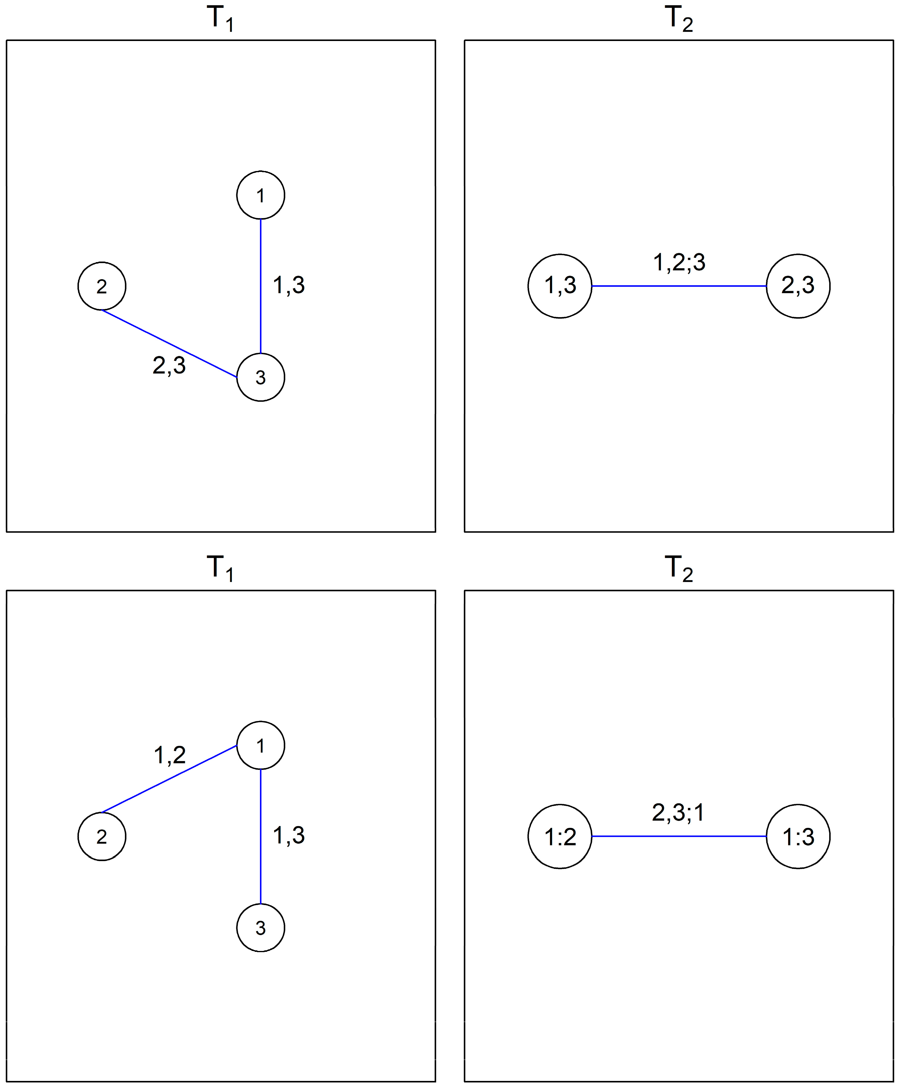
In this study, three possible vine trees sequence for the 3-dimensional case are considered. Figure 1 in Section 2 illustrates the first vine trees sequence. The other two vine trees sequences are presented in Figure 4. For the first vine trees sequence in the first row of Figure 4, the density for its simplified regular vine copula is

$$c\left(u_1,u_2,u_3\right)=c_{1,2:3}\left(C_{1|3}\left(u_1|u_3\right),C_{2|3}\left(u_2|u_3\right)\right)\times c_{1,3}\left(u_1,u_3\right)\times c_{2,3}\left(u_2,u_3\right).$$

(20)

Based on its vine trees sequence, this simplified regular vine copula also can be classified as a simplified canonical vine copula with a root nodes sequence $312$ and a simplified drawable vine copula with node order 132.

For the case of vine trees sequence at the second row, the density for its simplified regular vine copula is

$$c\left(u_1,u_2,u_3\right)=c_{2,3:1}\left(C_{2|1}\left(u_2|u_1\right),C_{3|1}\left(u_3|u_1\right)\right)\times c_{1,2}\left(u_1,u_2\right)\times c_{1,3}\left(u_1,u_3\right).$$

(21)

By looking at its vine trees sequence, the latter simplified regular vine copula also can be identified as a simplified canonical vine copula with a root nodes sequence $123$ and a simplified drawable vine copula with node order 213.

For the sake of simplicity in mentioning these vine copulas, by using the identity related to canonical vine copula, which is the root nodes sequence, the three simplified vine copulas mentioned in Equations (13), (20) and (21) are called $R\mathrm{v}213$, $R\mathrm{v}312$, and $R\mathrm{v}123$, respectively.

For every simplified vine copula ($R\mathrm{v}213$, $R\mathrm{v}312$, and $R\mathrm{v}123$), the appropriate copula model must be assigned to each component, including the pair copulas and a conditional pair copula. The determination process for finding an appropriate copula model for those components can be done independently. For that, the maximum likelihood estimation (MLE) and the Akaike information criteria (AIC) are applied to optimize the copula model’s parameters and to determine the most well-fitted pair copula (or conditional pair copula), respectively. Here, various parametric pair copula models are tested, all of which are listed in

Table 2. List of the tested parametric pair (or bivariate) copula models.

Number	Copula Short Name	Copula Long Name	Parameter Number
1	N	Gaussian	1
2	t	t	2
3	C	Clayton	1
4	G	Gumbel	1
5	F	Frank	1
6	J	Joe	1
7	BB1	BB1	2
8	BB6	BB6	2
9	BB7	BB7	2
10	BB8	BB8	2
11	SC	Survival Clayton	1
12	SG	Survival Gumbel	1
13	SJ	Survival Joe	1
14	SBB1	Survival BB1	2
15	SBB6	Survival BB6	2
16	SBB7	Survival BB7	2
17	SBB8	Survival BB8	2
18	Tawn	Tawn type 1	2
19	Tawn 180	180°-rotated Tawn type 1	2
20	Tawn 2	Tawn type 2	2
21	Tawn 2 180	180°-rotated Tawn type 2	2

. For conditional pair copula, $h$-functions that are similar to Equations (14) and (15) are first applied to obtain the relevant copula variables before the considered parametric pair copula models are tested.

Let two variables $u_{a,j}$ and $u_{b,j}$ such that $a,b\in \left\{1,2,3\right\}$ and $j=1,2,\cdots ,N$, the abovementioned MLE is determined by using the following formula

$$MLE=\underset{\theta \in \mathsf{\Theta }}{\max }\left\{\mathcal{l}\left(\theta ;\mathit{u}\right)\right\},$$

(22)

such that

$$\mathcal{l}\left(\theta ;\mathit{u}\right)=\prod _{\mathrm{j}=1}^N{c}_{a,b}\left(u_{a,j},u_{b,j};{\theta }_{a,b}\right),$$

(23)

where $\theta$ is the parameter of the possible set $\mathsf{\Theta }$. Whilst the abovementioned AIC is computed as follows

$$AIC=-2\sum _{\mathrm{j}=1}^N\mathrm{l}\mathrm{n}\left(c_{a,b}\left(u_{a,j},u_{b,j};{\theta }_{a,b}\right)\right)+2k,$$

(24)

where $k$ is the total number for the pair copula model’s parameters. Here, function BiCopSelect in R-package VineCopula is used for computation involving the selection of the best pair copulas and conditional pair copula [50].

Alternative to the MLE as defined in Equation (22), the inversion of Kendall’s $\tau$ correlation coefficient (Itau) can also be used to optimize the pair copulas and the conditional pair copula. By using the Itau, parameters $\theta$ are estimated using $\theta =C^{-1}\left(\widehat{\tau }\right)$, where $C^{-1}$ is the inverse function of the used pair copula model and $\widehat{\tau }$ is the empirical coefficient of Kendall’s $\tau$ correlation Correlation. However, the MLE is preferable compared to the Itau because it is more potent when the parameters in a model are few (e.g., one or two) and applicable to all pair copula models, as listed in Table 2.

Nevertheless, in this study, after all its components are determined, in the parametric setting, each simplified regular vine copula ($R\mathrm{v}213$, $R\mathrm{v}312$, and $R\mathrm{v}123$) is optimized using three methods, namely the sequential inversion of Kendall’s $\tau$ correlation coefficient (Seq-Itau), the sequential MLE (Seq-MLE), and the joint MLE (Joint-MLE). The first two optimizers share the same sequential strategy to estimate the parameters for a simplified vine copula.

For the sequential strategy, we can take an example of $R\mathrm{v}213$, where the parameters ${\theta }_{1,2}$, ${\theta }_{2,3}$, and ${\theta }_{1,3;2}$ that correspond to pair copulas $c_{1,2}$, $c_{2,3}$, and conditional pair copula $c_{1,3;2}$, respectively. can be sequentially optimized using the MLE or the Itau method. Following the vine trees sequence, parameters ${\theta }_{1,2}$ and ${\theta }_{2,3}$ are firstly optimized using the MLE or the Itau method. After that, the $h$-function is used to obtain copula variables related to the conditional pair copula $c_{1,3;2}$. Sequentially, the MLE or the Itau method is used once again to optimize the last parameter ${\theta }_{1,3;2}$. In this study, a function RVineSeqEst in R- package VineCopula is applied to fit the pair copulas and a conditional pair copula.

Staying with the same example of $R\mathrm{v}213$, Joint-MLE optimizes the parameter set $\mathit{\theta }=\left\{{\theta }_{1,2},{\theta }_{2,3},{\theta }_{1,3;2}\right\}$ by maximizing the joint likelihood for the triviate simplified regular vine copula $R\mathrm{v}213$, as defined below

$$\begin{gathered} \mathcal{l}\left(\mathit{\theta };\mathit{u}\right)=\prod _{\mathrm{j}=1}^N{c}_{1,3,2}\left(C_{1|2}\left(u_{j,1},u_{j,2};{\theta }_{1,2}\right),C_{3|2}\left(u_{j,3},u_{j,2};{\theta }_{2,3}\right);{\theta }_{1,3;2}\right) \\ \times c_{2,3}\left(u_{j,2},u_{j,3};{\theta }_{2,3}\right)c_{1,2}\left(u_{j,1},u_{j,2};{\theta }_{1,2}\right). \end{gathered}$$

(25)

For this study, the Joint-MLE approach is performed using the function RVineMLE in R-package VineCopula [48,51].

Therefore, for each simplified regular vine copula ($R\mathrm{v}213$, $R\mathrm{v}312$, and $R\mathrm{v}123$), which is optimized using Seq-Itau, Seq-MLE, or Joint-MLE, the log-likelihood, AIC, and BIC are used for model comparison purposes to determine the best model. Here, the best model is regarded as the model with the highest log-likelihood and the lowest AIC and BIC. In this study, the log-likelihood, AIC, and BIC are computed using R-package VineCopula through the functions RVineLogLik, RVineAIC, RVineBIC, respectively [50]. Furthermore, the Vuong tests are also applied to compare the fitting similarity of the models [52]. For these tests, if two models have a test statistical score with a significant $p$-value at 0.05 level ($p\le 0.05)$, then these two compared models are very similar in their model fitting. Here, the test statistic score and $p$-value of the Vuong tests are obtained from the function RVineVuongTest of R-package VineCopula [50].

Lastly, the Kendall’s $\tau$ correlation, upper tail dependence ${\lambda }^{\mathrm{upper}}$, and lower tail dependence ${\lambda }^{\mathrm{lower}}$ coefficients are also computed for the best model. Normally, the $d$-variate Kendall’s $\tau$ correlation coefficient of a multivariate copula $C$ is defined by [53]

$$\tau =\frac{2^d}{2^{d-1}-1}{\int }_{{\left[0,1\right]}^d}^{}CdC-\frac{1}{2^d}$$

(26)

For Equation (26), the value of Kendall’s $\tau$ correlation coefficient is given by $\tau \in \left[-\frac{1}{2^{d-1}-1},1\right]$, where $d$ is the dimension of a multivariate copula $C$. In addition, the $d$-variate upper tail dependence ${\lambda }^{\mathrm{upper}}$, and lower tail dependence ${\lambda }^{\mathrm{lower}}$ coefficients are, respectively, defined by

$${\lambda }^{\mathrm{upper}}=\underset{\mathit{t}\to 1^{-1}}{\lim }\frac{C\left(1-\mathit{t}\right)}{1-C\left(\mathit{t}\right)}$$

(27)

and

$${\lambda }^{\mathrm{l}\mathrm{o}\mathrm{w}\mathrm{e}\mathrm{r}}=\underset{\mathit{t}\to 0^{+}}{\lim }\frac{C\left(\mathit{t}\right)}{1-C\left(1-\mathit{t}\right)}$$

(28)

where $\mathit{t}=\left(t,t,\cdots ,t\right)$, $1-\mathit{t}=\left(1-t,1-t,\cdots ,1-t\right)$ and $\widehat{C}$ is the survival copula of a multivariate copula $C$ [54]. For every $d$-multivariate copula $C$, we have ${\lambda }^{\mathrm{upper}},{\lambda }^{\mathrm{l}\mathrm{o}\mathrm{w}\mathrm{e}\mathrm{r}} \in \left[0,1\right]$.

However, due to simplicity and ease of computing, in this study, the used formulas for Kendall’s $\tau$ correlation, upper tail dependence ${\lambda }^{\mathrm{upper}}$ and lower tail dependence ${\lambda }^{\mathrm{lower}}$ coefficients, respectively, are

$$\tau =\frac{1}{\left(\begin{array}{c}d\\ 2\end{array}\right)}{\sum }_{r\ne s}^{}{\tau }_{r,s}$$

(29)

$${\lambda }^{\mathrm{upper}}=\frac{1}{\left(\begin{array}{c}d\\ 2\end{array}\right)}{\sum }_{r\ne s}^{}{\lambda }_{r,s}^{upper},$$

(30)

and

$${\lambda }^{\mathrm{lower}}=\frac{1}{\left(\begin{array}{c}d\\ 2\end{array}\right)}{\sum }_{r\ne s}^{}{\lambda }_{r,s}^{lower}$$

(31)

where ${\tau }_{r,s}$, ${\lambda }_{r,s}^{upper}$, ${\lambda }_{r,s}^{lower}$ are the Kendall’s $\tau$ correlation coefficient of pair copula or conditional pair copula for variables $U_r,U_s$, as defined in Equations (6)–(8), respectively [55]. Kendall’s $\tau$ correlation coefficient will lie down in the range $\left[-1,1\right],$ since every ${\tau }_{r,s}\in \left[-1,1\right]$. For the upper tail dependence ${\lambda }^{\mathrm{upper}}$ and lower tail dependence ${\lambda }^{\mathrm{lower}}$ coefficients, they are in the range $\left[0,1\right]$ since the probabilities ${\lambda }_{r,s}^{upper},{\lambda }_{r,s}^{lower}\in \left[0,1\right]$.

For a vine copula model, these coefficients of Equations (29)–(31) can be used to measure the central dependency, the probability of the joint occurrence of extremely large values, and the probability of the joint occurrence of extremely small values for the best model. The last two coefficients are also used to determine whether the best model is asymmetric or not. Furthermore, to aid our analysis on its dependencies, the tractable property of the vine copula model is also used, where the figures of its pair copulas are observed to provide useful and clearer insights into our vine copula model.

5. Result

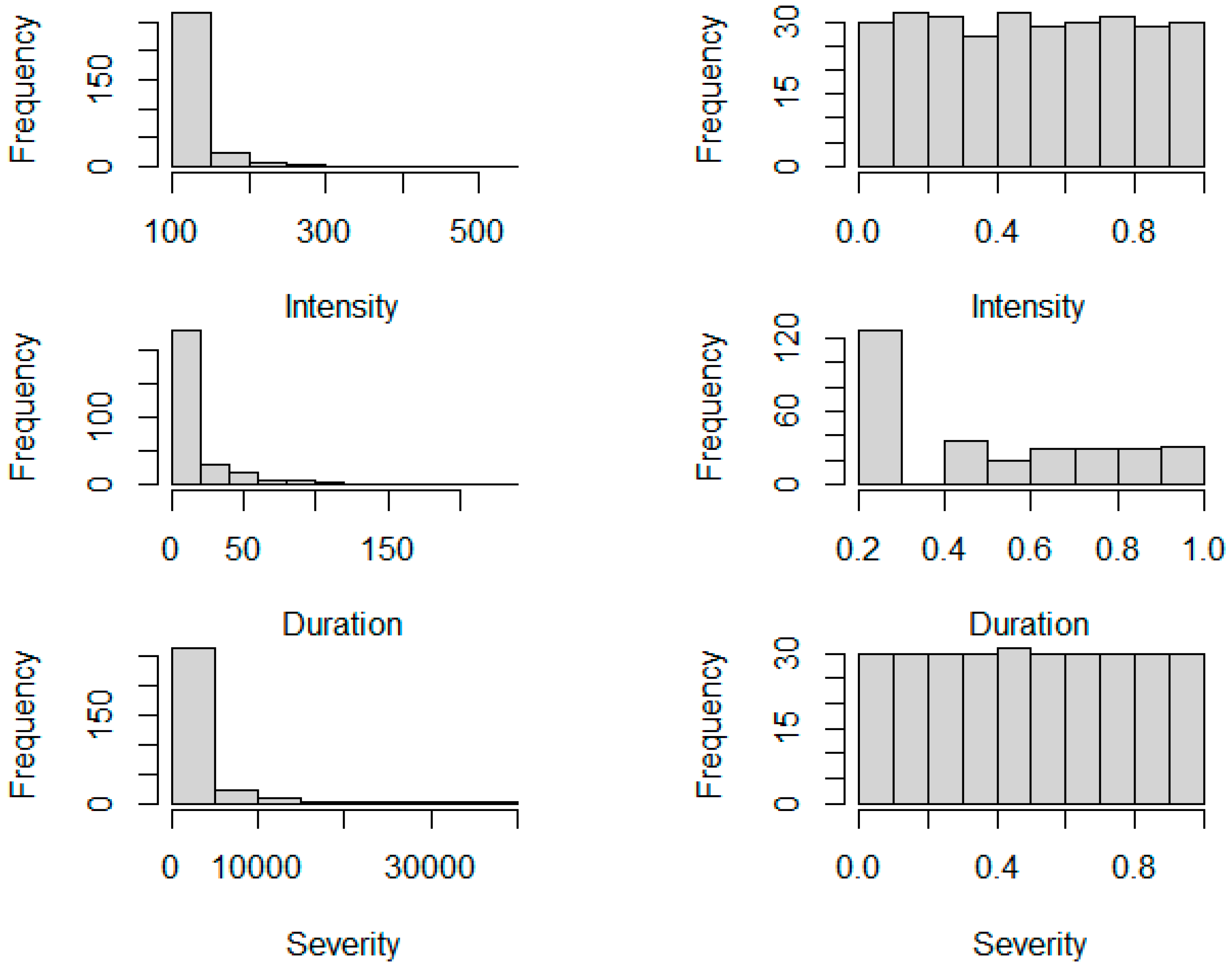
In this study, simplified vine copula models are applied to examine the characteristics of unhealthy events, namely intensity, duration, and severity. Prior to the modeling, data in the original scale is transformed into new data in the copula scale by using the PIT approach, as mentioned in the first paragraph of Section 4. Marginal histograms for the original data (in the first column) and copula data (in the second column) are presented in Figure 5. The latter data follow a uniform pattern as compared to the previous data, resulting from the PIT transformation. This implies that the dependence structure is now independent of marginal effects.

From there, a preliminary analysis is done using the obtained copula data. The results of this analysis, consisting of marginal histograms, pair plots, Kendall’s $\tau$ correlation coefficients, and empirical contour plots are provided in Figure 6. Behaviors on marginal histograms at the diagonal of Figure 6 have been discussed in the above paragraph. In Figure 6, focusing on the pair plots and Kendall’s $\tau$ correlation coefficients (located above the diagonal), all the pairs show positive relationships. The stronger correlation of 0.89 is indicated by the relationship between severity and duration. This follows by the pair of variables, between intensity and severity (0.55), and the duo of variables, between intensity and duration (0.39). A higher correlation indicates that the pair has a more similar rank between two variables, such as increases in air pollution severity being more likely to happen because of a prolonged unhealthy event. Besides that, normalized contour plots also indicate a similar pattern, where all pairs are in a non-elliptical shape, indicating that an elliptical distribution is not favorable here.

Consequently, all three simplified regular vine copulas ($R\mathrm{v}213$, $R\mathrm{v}312$, and $R\mathrm{v}123$) are considered to model a tri-variate dependence structure for the severity, intensity, and duration relationship. In doing that, components for each considered simplified regular vine copula, such as the pair copulas and a conditional pair copula, need to be determined. In this study, the pair copulas and a conditional pair copula are modeled using various parametric bivariate copula models, listed in Table 2. At this point, the MLE, the AIC, and $h$-function are used to fit the model, to choose the appropriate model, and to obtain pseudo copula data for the conditional pair copula prior to the modeling, respectively.

Table 3. The appropriate models for pair copulas and conditional pair copula of a simplified regular vine copula $R\mathrm{v}213$.

Tree	Copula	Pair	Term	The Best Model	Par	Par2	Tau	Ltd	Utd
1	Pair copula	(Int, Dur)	$c_{,1:2}$	Tawn type 1	2.62	0.42	0.32	0.00	0.39
1	Pair copula	(Dur, Sev)	$c_{2,3}$	Joe	11.81	-	0.85	0.00	0.94
2	Conditional pair copula	(Int, Sev; Dur)	$c_{1,3:2}$	Rotated BB8 270 degrees	−6.00	−0.73	−0.55	0.00	0.00

,

Table 4. The appropriate models for pair copulas and conditional pair copula of a simplified regular vine copula $R\mathrm{v}312$.

Tree	Copula	Pair	Term	The Best Model	Par	Par2	Tau	Ltd	Utd
1	Pair copula	(Int, Sev)	$c_{,1:3}$	Rotated Tawn type 1 180 degrees	4.70	0.58	0.49	0.56	0.00
1	Pair copula	(Dur, Sev)	$c_{2,3}$	Joe	11.81	-	0.85	0.00	0.94
2	Conditional pair copula	(Int, Dur; Sev)	$c_{1,2:3}$	Rotated BB8 270 degrees	−5.68	−0.80	−0.58	0.00	0.00

and

Table 5. The appropriate models for pair copulas and conditional pair copula of a simplified regular vine copula $R\mathrm{v}123$.

Tree	Copula	Pair	Term	The Best Model	Par	Par2	Tau	Ltd	Utd
1	Pair copula	(Int, Dur)	$c_{,1:2}$	Tawn type 1	2.62	0.42	0.32	0.00	0.39
1	Pair copula	(Int, Sev)	$c_{1,3}$	Rotated Tawn type 1 180 degrees	4.70	0.58	0.49	0.56	0.00
2	Conditional pair copula	(Dur, Sev; Int)	$c_{2,3:1}$	Survival Gumbel	3.09	-	0.68	0.75	0.00

present the result of modeling the pair copulas and a conditional copula for simplified regular vine copulas $R\mathrm{v}213$, $R\mathrm{v}312$, and $R\mathrm{v}123$, accordingly.

For example, in Table 3, there are two pseudo copula data that are required before the conditional pair copula modeling. These pseudo copula data $C_{1|2}\left(u_1|u_2\right)$ and $C_{3|2}\left(u_3|u_2\right)$ can be obtained using the $h$-function such that

$$C_{1|2}\left(u_1|u_2\right)=h_{1|2}\left(u_1|u_2\right)=\frac{\partial }{\partial u_2}{C}_{12}\left(u_1,u_2\right),$$

(32)

and

$$C_{3|2}\left(u_3|u_2\right)=h_{3|2}\left(u_3|u_2\right)=\frac{\partial }{\partial u_2}{C}_{32}\left(u_3,u_2\right).$$

(33)

After that, by using the pseudo copula data $C_{1|2}\left(u_1|u_2\right)$ and $C_{3|2}\left(u_3|u_2\right)$, the MLE, and the AIC, the most well-fitted conditional pair copula model is determined. Consequently, Kendall’s $\tau$ correlation, upper tail dependence ${\lambda }^{\mathrm{upper}}$, and lower tail dependence ${\lambda }^{\mathrm{lower}}$ coefficients of the conditional pair copula (as mentioned in the third row of Table 3) can be computed using Equations (6)–(8), respectively. The same procedure is also applied to compute Kendall’s $\tau$ correlation, upper tail dependence ${\lambda }^{\mathrm{upper}}$, and lower tail dependence ${\lambda }^{\mathrm{lower}}$ coefficients of the conditional pair copula, as mentioned in the third row of Table 4, Table 5 and Table 7.

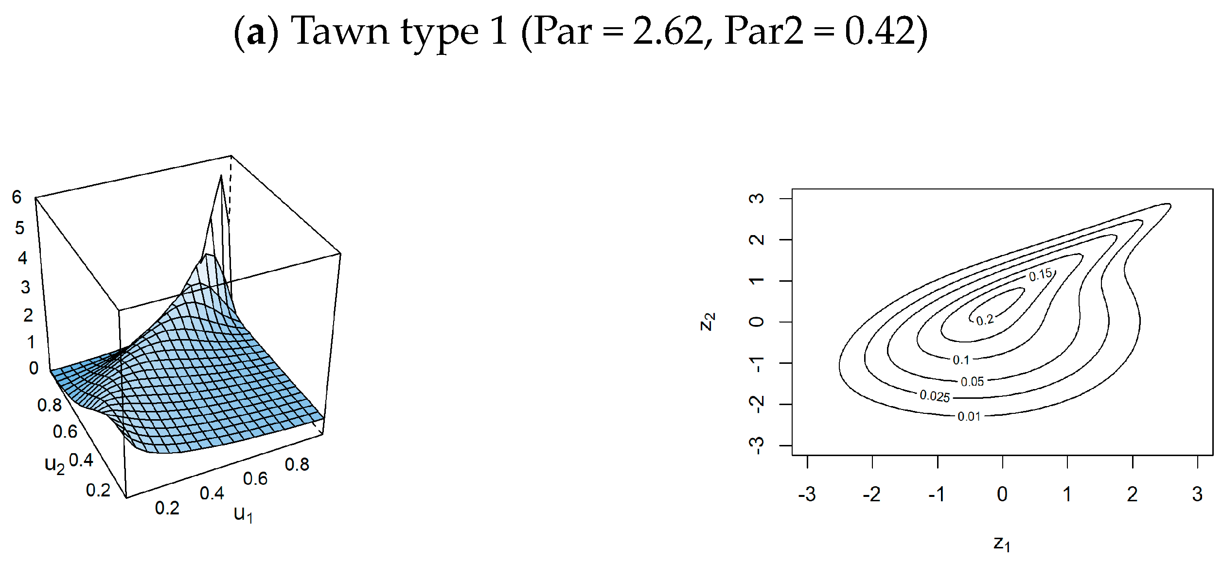
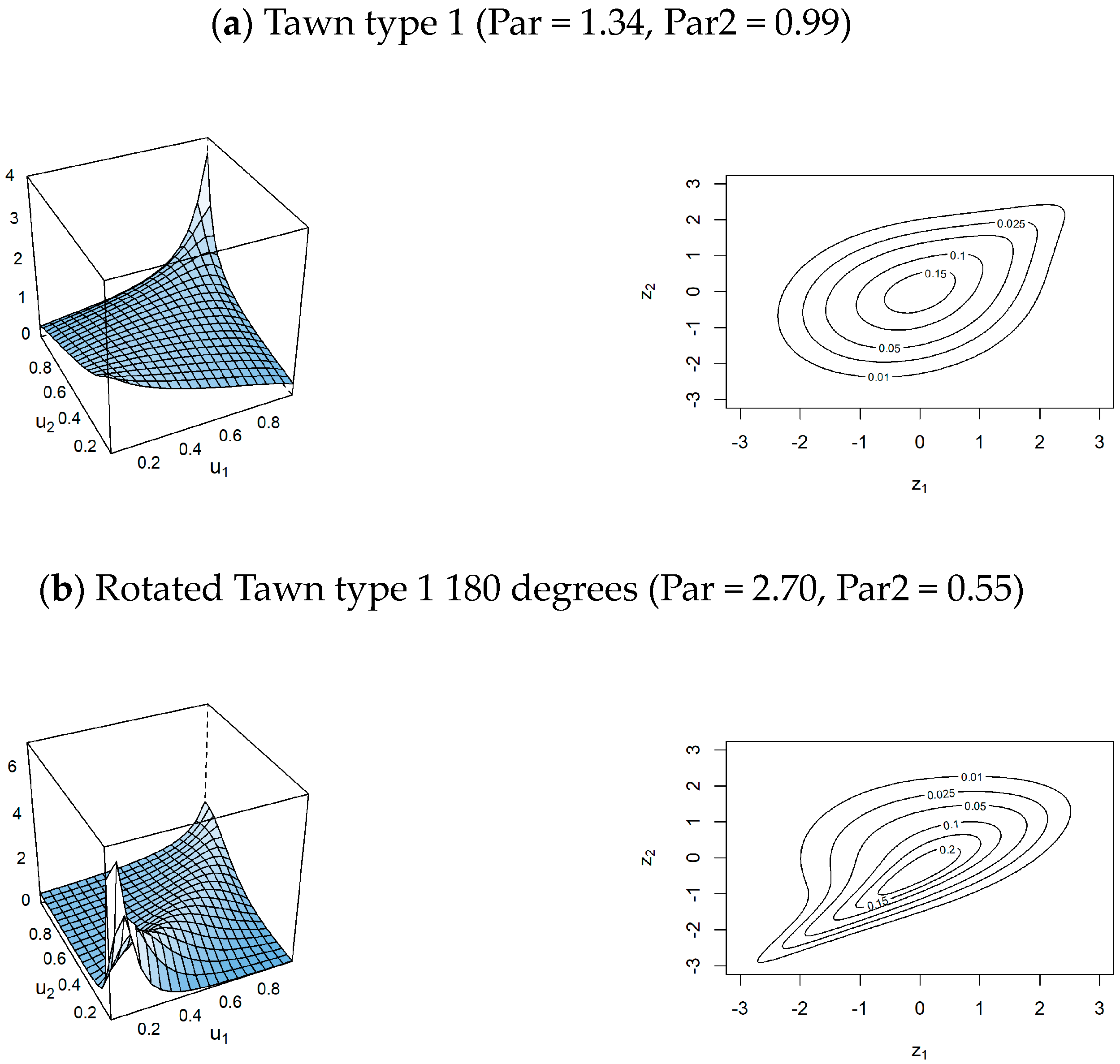
Based on Table 3, Table 4 and Table 5, for pair copulas, the well-fitted models for describing the dependence structure of the pairs of (intensity, severity), (duration, severity), and (intensity, duration) are the Tawn type 1, Rotated Tawn type 1 180 degrees, and Joe, respectively. This result is aligned with the outcome of [35]. The density and contour plots of these copulas are illustrated accordingly in Figure 7.

In Figure 7 (similar to Figure 8 and Figure 10), the variables $Z_1$ and $Z_2$ in the contour plots of the fitted conditional pair have a marginally normalized scale, where $Z_{\mathrm{i}}={\Phi }^{-1}\left(U_i\right)={\Phi }^{-1}\left(F_i\left(X_i\right)\right)$ for $i=1,2$ with density $g\left(z_1,z_2\right)=c\left(\Phi \left(z_1\right),\Phi \left(z_2\right)\right)\varphi \left(z_1\right)\varphi \left(z_2\right)$. Here, $X_1$ and $X_2$ are original variables, while $U_1$ and $U_2$ are copula variables, such that $U_i=F_i\left(X_i\right)$. Furthermore, $c\left(·,·\right)$ is a copula density, and $\Phi \left(·\right)$ and $\varphi \left(·\right)$ are the distribution and density functions of a $N\left(0,1\right)$ variable.

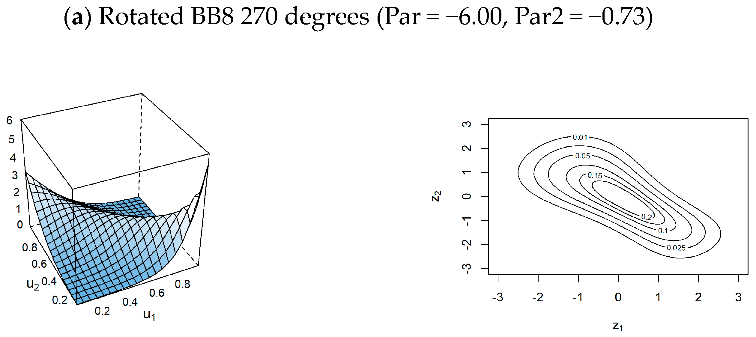
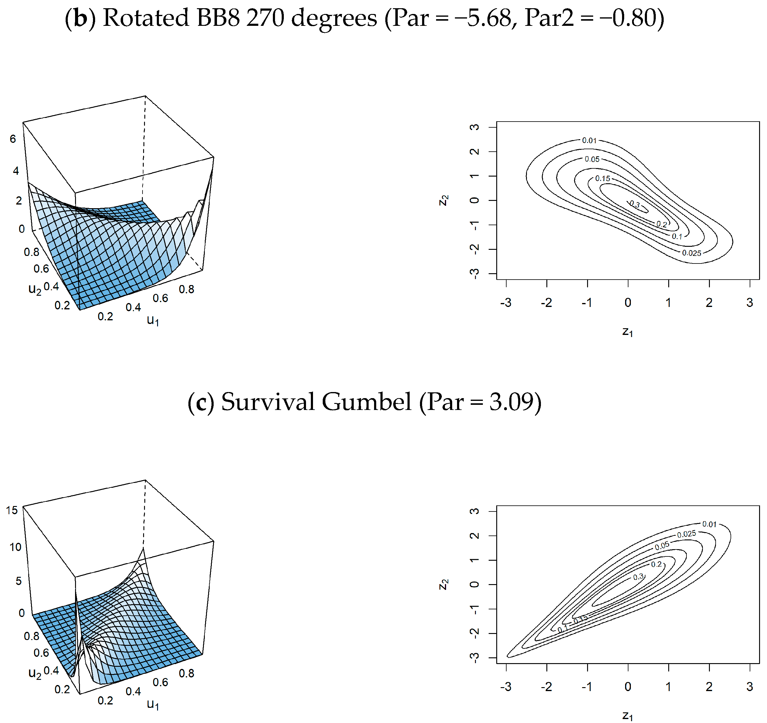
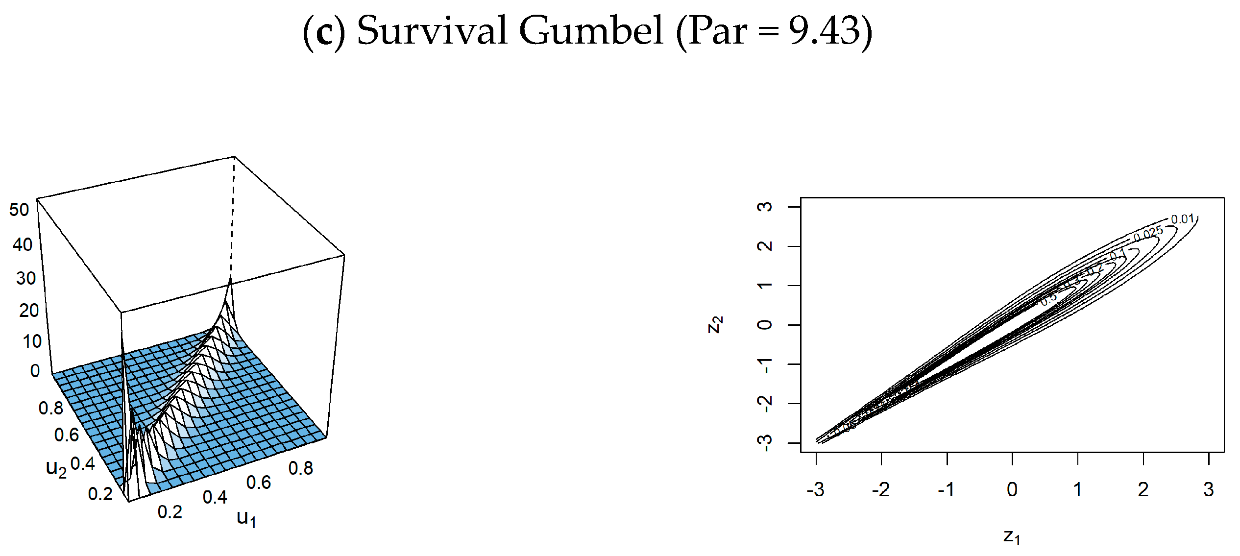
In addition, for the conditional cases, the conditional pairs of (intensity, severity; duration), (intensity, duration; severity) are better modeled by the Rotated BB8 270 degrees, while (duration, severity; intensity) is most appropriately modeled by the Survival Gumbel. For these conditional pair copulas, Figure 8 displays their density and contour plots, respectively.

Furthermore, for the conditional cases, there exist two cases where the obtained Kendall’s $\tau$ correlation coefficients are negative. These cases are the conditional pairs of (intensity, severity; duration) and (intensity, duration; severity) with Kendall’s $\tau$ correlation coefficient of −0.55 and −0.58, as reported in Table 3 and Table 4, respectively. For (duration, severity; intensity), Kendall’s $\tau$ correlation coefficient is positive (0.68), see Table 5. To interpret this value, for (intensity, severity; duration), the negative value (−0.55) shows that, conditional on the duration, the intensity and severity have inverse correlation, see Figure 8a. This indicates that while the intensity increases, the severity decreases, conditional on the duration. This interpretation is also held for (intensity, duration; severity). For a positive value like in (duration, severity; intensity), the duration and severity move in the same direction, conditional on the intensity. Therefore, conditional on the intensity, a positive correlation (0.68) indicates that duration and severity tend to increase (or decrease) together, see Figure 8c.

Focusing on Figure 7 and Figure 8, despite pair and conditional pair copulas, the most well-fitted copula models imply skewed distributions, except for the Rotated BB8 270 degrees in modeling the conditional pair copula models of (intensity, severity; duration) and (intensity, duration; severity). A skewed distribution is a distribution with one tail being longer than the other. This also leads to an asymmetrical distribution, the opposite shape to the familiar symmetric normal distribution with its bell-shaped curve. This aspect can be recognized based on their upper tail dependence, and lower tail dependence coefficients, where most of the models have different values between those two coefficients. For the Rotated BB8 270 degrees, both its coefficients (upper tail and lower tail dependences) are zero for the conditional pair copula models of (intensity, severity; duration) and (intensity, duration; severity), which indicates the possibility of a symmetry distribution. However, based on the first two rows in Figure 8, the observation on the density and contour plots show that the Rotated BB8 270 degrees for the conditional pair copula models of (intensity, severity; duration) and (intensity, duration; severity) are only approximate to the symmetry distribution because their tails (on the left and right) do not fully have the same dependence structure, although they look quite similar.

In addition, (lower and upper) tail dependencies are also dependent measures for the (small and large) extremes of a conditional pair copula model. For instance, let us take a conditional pair copula model of (intensity, severity; duration). If its (lower and upper) tail dependencies are zero, this also indicates that (small and large) extreme events such as air pollution with (small and large) extreme intensity and severity, conditional on the duration, are unlikely to happen. The same interpretation is also applicable to describe improbable extreme events like air pollution with (small and large) extreme intensity and duration, conditional on the severity.

Consequently, the obtained models for pair and conditional pair copulas are applied accordingly as component structures to three different vine trees sequences, as depictured in Figure 1 and Figure 4, to construct simplified regular vine copulas $R\mathrm{v}213$, $R\mathrm{v}312$, and $R\mathrm{v}123$, respectively. Then, these simplified regular vine copulas are optimized using three different approaches, namely Seq-Itau, Seq-MLE, or Joint-MLE. For simplicity, the nine different simplified vine copula models tested in this study are named as Rv213-Seq-Itau, Rv213-Seq-MLE, Rv213-Joint-MLE, Rv312-Seq-Itau, Rv312- Seq-MLE, Rv312-Joint-MLE, Rv123-Seq-Itau, Rv123-Seq-MLE, Rv123-Joint-MLE. In this study, these simplified regular vine copula models are combined in terms of model fitting, where the best model is concluded to have the highest log-likelihood estimate and the lowest AIC and BIC scores.

Table 6. The obtained results of the loglikelihood, AIC, and BIC for all nine simplified regular vine copulas.

Models	Log-Likelihood	AIC	BIC
Rv213-Seq-Itau	461.26	−912.53	−893.99
Rv213-Seq-MLE	482.13	−954.27	−935.73
Rv213-Joint-MLE	496.95	−983.90	−965.36
Rv312-Seq-Itau	605.20	−1200.40	−1181.87
Rv312- Seq-MLE,	635.31	−1260.61	−1242.08
Rv312-Joint-MLE	662.92	−1315.84	−1297.30
Rv123-Seq-Itau	391.29	−772.57	−754.04
Rv123- Seq-MLE	434.99	−859.99	−841.45
Rv123-Joint-MLE	672.22	−1334.44	−1315.90

presents the obtained results of the loglikelihood, AIC, and BIC for all nine simplified regular vine copulas.

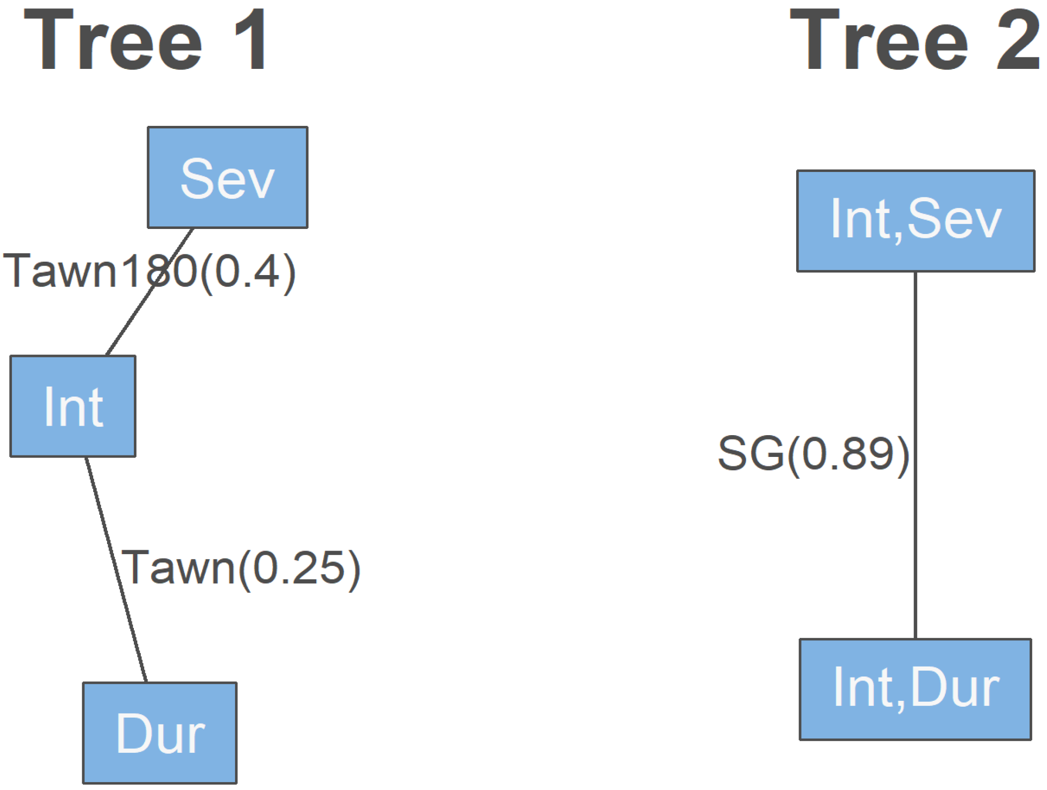
Based on Table 6, by observing the values of the loglikelihood, AIC, and BIC, the best method to optimize a simplified vine copula model is Joint-MLE, followed by Seq-Itau, and Seq-MLE. Despite the dissimilarity of the simplified vine copula models, as compared to other optimizers, Joint-MLE provides the highest log-likelihood estimate and the lowest AIC and BIC scores. Overall, as bolded in Table 6, Rv123-Joint-MLE is identified as the best simplified regular vine copula to model the tri-variate dependence structure of intensity, duration, and severity. This identification is also based on the highest log-likelihood (672.22) and the lowest AIC (−1334.44) and BIC (−1315.90) scores achieved by this model. The vine trees sequence for the best model Rv123-Joint-MLE is illustrated in Figure 9.

Furthermore, the details regarding the component structures, consisting of the pair copulas and a conditional pair copula of the best model Rv123-Joint-MLE, are also provided in

Table 7. The appropriate models for pair copulas and conditional pair copula of the best model Rv123-Joint-MLE.

Tree	Copula	Pair	Term	The Best Model	Par	Par2	Tau	Ltd	Utd
1	Pair copula	(Int, Dur)	$c_{,1:2}$	Tawn type 1	1.34	0.99	0.25	0.92	0.00
1	Pair copula	(Int, Sev)	$c_{1,3}$	Rotated Tawn type 1 180 degrees	2.70	0.55	0.40	0.48	0.00
2	Conditional pair copula	(Dur, Sev; Int)	$c_{2,3:1}$	Survival Gumbel	9.43	-	0.89	0.00	0.32

. Additionally, the density and contour plots for these pairs and the conditional pair copulas of the best model Rv123-Joint-MLE are also displayed in Figure 10. From Figure 10, all the component structures illustrate skewness in their density curves. This skewness is also demonstrated by the dissimilarity between the coefficients of the upper tail and lower tail dependencies, as shown in the first and second last columns of Table 7. In addition, by comparing Table 5 and Table 7, it is worth noting that that the optimizer Joint-MLE (Table 7) indeed provides different optimized parameters, as compared to the optimizer Seq-MLE (Table 5). Therefore, parameters obtained from the optimizer Joint-MLE are better for fitting the component structures of a simplified regular vine copula model.

Furthermore, by using Equations (29)–(31), Kendall’s $\tau$ correlation Correlation, upper tail dependence ${\lambda }^{\mathrm{upper}}$, and lower tail dependence ${\lambda }^{\mathrm{lower}}$ coefficients for the best model Rv123-Joint-MLE are 0.51, 0.47, and 0.11, respectively. For unhealthy events, Kendall’s $\tau$ correlation coefficient for the best model Rv123-Joint-MLE indicates that the intensity, duration, and severity have a positive monotonous relation among them (0.51), implying the existence of chance that these three characteristics (intensity, duration, and severity) increase together. Moreover, based on the dissimilarity in the upper tail dependence ${\lambda }^{\mathrm{upper}}$ (0.47), and lower tail dependence ${\lambda }^{\mathrm{lower}}$ (0.11) coefficients for the best model Rv123-Joint-MLE, this model also demonstrates that the dependence structure of the severity, intensity, and duration relationship is skewed and follows asymmetric distribution patterns. In addition, as illustrated in Figure 10, the components of the best model Rv123-Joint-MLE are dissimilar at their tail parts and these facts also support the finding that the dependence structure of the severity, intensity, and duration relationship is skewed and follows asymmetric distribution patterns.

On the other hand, a comparison study based on the Vuong tests is also used to investigate significant evidence to distinguish the best model Rv123-Joint-MLE from other models. Results obtained from comparing Rv123-Joint-MLE with other models are reported in

Table 8. Results from the Vuong tests comparing the best model Rv123-Joint-MLE with other models.

Comparison	Stat	$\mathit{p}$-Value	Stat-AIC	$\mathit{p}$-Value	Stat-BIC	$\mathit{p}$-Value
Rv213-Seq-Itau	−6.18	0.00	−6.18	0.00	−6.18	0.00
Rv213-Seq-MLE	−6.93	0.00	−6.93	0.00	−6.93	0.00
Rv213-Joint-MLE	−6.38	0.00	−6.38	0.00	−6.38	0.00
Rv312-Seq-Itau	−2.23	0.03	−2.23	0.03	−2.23	0.03
Rv312- Seq-MLE	−1.57	0.12	−1.57	0.12	−1.57	0.12
Rv312-Joint-MLE	−0.44	0.66	−0.44	0.66	−0.44	0.66
Rv123-Seq-Itau	−7.15	0.00	−7.15	0.00	−7.15	0.00
Rv123- Seq-MLE	−8.83	0.00	−8.83	0.00	−8.83	0.00

. By using the Vuong tests at the 5% level, this comparison study shows that the best model Rv123-Joint-MLE is significantly different from others, whereas some are quite similar. The Vuong tests indicate that there is significant evidence that the best model Rv123-Joint-MLE is different from Rv213-Seq-Itau, Rv213-Seq-MLE, Rv213-Joint-MLE, Rv312-Seq-Itau models, which indicates that the best model is superior to them. Alternatively, there is no significant evidence to show that the best model Rv123-Joint-MLE is dissimilar with Rv312-Seq-MLE and Rv312-Joint-MLE, which signifies that the probability of a closely similar dependence structure among these three latter models. Therefore, using the three latter models may result in similar insight into air pollution data, especially to the tri-variate dependence structure of the three characteristics studied here, namely intensity, duration, and severity.

6. Conclusions

Focusing on the unhealthy events, this study applied the vine copula approach to model the tri-variate dependence structure of three air pollution characteristics, namely intensity, duration, and severity. The vine copula approach is a more reliable, realistic, flexible, and tractable model than the standard multivariate distributions, and multivariate copulas, especially in modeling the tail behaviors related to extreme events. Klang was chosen as the study area because its exposure rate is higher than other major cities in Malaysia. In this study, three vine copulas with different vine trees sequence, namely $R\mathrm{v}213$, $R\mathrm{v}312$, and $R\mathrm{v}123$ were analyzed and compared based on their model fitting and a comparison of the models.

In modeling each vine copula, the MLE and AIC were first applied to identify the best parametric bivariate model for all the vine copula components, including the pair copulas and a conditional pair copula. The $h$-function was also applied to obtain pseudo copula data before searching for the best associated parametric bivariate model. After that, each vine copula model was optimized using three different optimizers, namely Seq-Itau, Seq-MLE, and Joint-MLE. As a result, there were nine methods examined, called Rv213-Seq-Itau, Rv213-Seq-MLE, Rv213-Joint-MLE, Rv312-Seq-Itau, Rv312- Seq-MLE, Rv312-Joint-MLE, Rv123-Seq-Itau, Rv123- Seq-MLE, Rv123-Joint-MLE.

For model fitting, the log-likelihood estimate, and AIC and BIC scores were used to compare those models and determine the best model. Here, the best model was identified by the highest log-likelihood and the lowest AIC and BIC scores. Furthermore, the Vuong tests at the 5% level were applied to compare the best model with other models, in terms of fitting similarity between the two compared models.

This study showed that the best model was Rv123-Joint-MLE, a model with a root nodes sequence of 123 and optimized using the Joint-MLE. For its components, the Tawn type 1 and Rotated Tawn type 1 180 degrees were selected for modeling pair copulas of (intensity, duration) and (intensity, severity), respectively. For the conditional pair copula (duration, severity; intensity) was modeled by the Survival Gumbel. All these components were skewed and not distributed symmetrically. Furthermore, the best model Rv123-Joint-MLE demonstrated that the dependence structure of severity, intensity, and duration relationship was positively correlated, skewed and followed an asymmetric distribution. For the comparison study, the best model was found to be significantly different from the others, whereas some were quite similar.

The practical use of the proposed model Rv123-Joint-MLE is to be used as a tool to measure the risks of extreme events. To do this, a simulation of the proposed model Rv123-Joint-MLE can be applied to obtain the stimulated copula variables. After that, by using the discrete inverse sampling approach, the stimulated copula variables are transformed into the original variables. Empirically, some probability measures related to extreme events can be computed. These measures include the conditional probability of extreme events, the joint return period of extreme events, and the conditional return period measures for extreme events. Information obtained from these measures can be leveraged by policymakers or regulators to assess the risk of extreme air pollution events and take the necessary action to possibly avoid the worse effects of such events and sustain clear air for public well-being. Overall, this paper highlights the capability of vine copula in modeling the asymmetric dependence structure of air pollution characteristics (intensity, duration, and severity) and its potential to be used as a tool to measure risks of extreme events in future work.