Abstract
Since the droughts of the 1970s–1980s, populations in the Sahel region have opted for a mass exodus to more humid urban or rural centers. Migrations or exoduses have accelerated in recent decades due to environmental degradation and unfavorable climatic conditions. Insufficient harvests are the main reason for migration for the majority of migrants in the Sahelian areas. Migration is a major adaptation strategy to cope with extreme climatic conditions, thus requiring quantification in the destination area. The aim of this paper is to propose a metapopulation model to approximate reality by identifying the transition from one socioeconomic vulnerability group to another, from a less favorable area to favorable area in terms of natural resources, depending on the strategies, policies, and climate variability. The model was used to analyze the dynamics of socioeconomic vulnerability to study the impact of migration on the dynamics of socioeconomic vulnerability. The developed mathematical model was analyzed. Up to 2050, simulations applied to the Tougou village in northern Burkina Faso show that migration has a positive impact on the socioeconomic vulnerability of the destination area, thereby reducing the vulnerability of the population by 10% when resources are increased by up to 30%.
Keywords:
socioeconomic vulnerability; Sahel; metapopulation model; climate change; migration; Burkina Faso; nonlinear ordinary differential equation MSC:
34A34; 34C60; 34D20
1. Introduction
The Sahel region is characterized by economic, social, environmental, and political challenges that impact population movements. The movement of a person or group of people, either between countries or within a country between two locations (villages, towns, etc.), is viewed as migration [1]. Migrants’ destinations depend on a number of factors, such as climate change, conflicts, job seeking, economic reasons, etc. Depending on the reasons, migration may be periodic or permanent [2].
Well-planned and well-managed migration policies are one of the Sustainable Development Goals (SDGs). Indeed, target 10.7 of the goal aims to “reduce inequalities within and between countries” and makes central reference to migration, wherein it calls for “orderly, safe, regular and responsible migration and mobility, especially through the implementation of well-managed and planned migration policies” [3]. In the early 21st century, the volume of human mobility worldwide has reached an unprecedented level (around 258 million people, representing 3.4% of the world’s population, 48% of whom are women), as evidenced by the various migratory movements currently taking place throughout Latin America, Europe, and the Middle and Near East [4].
Africa, particularly Sub-Saharan Africa, has experienced significant migratory movements. Whether voluntary or forced, these movements are deeply rooted in the previous history of the continent [5,6]. Migration is viewed as an adaptation strategy to climate change in the Sahel region [7]. Indeed, populations move to areas to reduce their socioeconomic vulnerability. Major population movements are taking place from the northern regions of the Sahel towards the south and coastal countries. Sahelian migrants move to rural or urban areas in their own countries or abroad. The host areas are coastal countries, mainly Côte d’Ivoire—because of its cocoa plantations—Nigeria, and Ghana—which is a former host country whose recent prosperity is once again attracting Sahelians [8]. Intracountry migration affects less populated rural areas with higher rainfall, such as Casamance and the new lands of Senegal, as well as the cotton-growing areas of southern Burkina Faso and Mali [9].
The causes of population migration in the Sahel are numerous, complex, and often result from the interaction of economic, environmental, political, and social factors. Studies have shown that inhabitants of drier regions are more likely to engage in temporary and permanent migration to other rural areas than those in wetter regions [10]. Short-term rainfall deficits tend to increase the risk of long-term migration to rural areas and decrease the risk of short-term migration to distant destinations [10]. High demographic pressure on natural resources is considered to be the major cause of migration in the Sahel [11,12,13]. The unfriendly climate is progressively pushing Sahelians towards the rainier south [9,14,15,16]. From the literature review, we note that extreme poverty and political instability increase migration to more peaceful areas where employment opportunities are high [17]. The increasing frequency and severity of climate-related disasters such as floods and droughts can lead to more permanent migration over time. Urbanization can bring about migratory movements from the countryside to the cities [18].
Based on the causes of migration, we define the types of migration as follows: (i) economic migration, which involves the movement of people in search of better economic opportunities; (ii) forced migration, which is due to conflict and insecurity; (iii) climatic migration, which is associated with the movement of populations in response to increasingly difficult environmental conditions such as the loss of agricultural land or water scarcity; (iv) seasonal migration, which generally involves nomadic herders who migrate with their flocks/herds according to the seasons to gain access to suitable pastures and water resources; (v) rural–urban migration, which is related to the process of growing urbanization in search of jobs, education, and better living conditions; (vi) return migration, which occurs after having worked or lived abroad or in other parts of the country, where some migrants choose to return to their region of origin; (vii) crossborder migration, which is recurrent and occurs between countries in the subregion for economic, climatic, or cultural reasons; and (viii) mixed migration, which involves a combination of motives, such as job seeking, escaping from conflict, etc. [19,20,21,22,23].
Assessing the impact of migration on the socioeconomic vulnerability of the Sahelian population often requires a variety of models and methodologies to understand and predict migration trends. The various models that are commonly used to assess migration in the Sahel region include the following: (i) gravity models, which are based on the theory of economic gravity and assess migration flows on the basis of the size and distance between sending and receiving regions/departing and host regions; (ii) regression models, which use independent variables, such as income, education, employment, and other socioeconomic factors to predict the probability/likelihood of migration; (iii) simulation models, which simulate the impacts of various factors, including climate change or migration patterns over time; (iv) GIS (geographic information system)-based models, which are used to map migration trends by using geographic data to visualize population movements; (v) scenario models, which are used to explore different possible migration trajectories under different socioeconomic and environmental scenarios; (vi) integrated models, which combine several approaches to assess migration in the Sahel; they often integrate elements such as demographic, economic, environmental, and political data to provide a more comprehensive overview of migration trends; and (vii) social network models, which focus on the social and family networks that influence migration decisions [24,25,26,27,28,29,30]. Among these models, we have not encountered in the literature a mathematical model of the metapopulation type that takes into account the migration of populations from a less-resourced area to a more-resourced one to assess the socioeconomic vulnerability of the destination area.
This model is based on the model developed in [31], which has already taken into account the socioeconomic vulnerability dynamics of Sahelian populations, without integrating the migration between zones. Migration plays a key role in adaptation strategies to climate variability, and the metapopulation model will quantify the impact of migration in an area with favorable natural resource conditions.
In the literature, there several definitions of the metapopulation, which generally depend on the nature of the movements between localities (subpopulation or patches). These models have been developed to model the spatiotemporal dynamics of communicable diseases (see [32,33,34,35,36]). A metapopulation model involves explicit movements of individuals between different localities.
Section 2 presents the socioeconomic and climatic data used to simulate the model. Section 3 formulates the metapopulation model, whereas Section 4 and Section 5 deal respectively with the existence, the uniqueness of the solution of the nonlinear differential equation system formulated, and the determination of the basic reproduction number followed by the stability. As for the penultimate Section 6, it examines the results of simulations that will allow us to see the impact of migration applied to two zones, one of which is favorable in terms of resources and the other unfavorable in terms of resources. Finally, the last Section 7 represents the conclusion of our study.
2. Data
Four socioeconomic surveys were carried out among the heads of households in Tougou. Tougou is a village located in the northern region of Burkina Faso, specifically within the province of Yatenga (see Figure 1). These surveys took place after the harvest in the village in 2004, 2006, 2008, and 2010. The same households were surveyed in all four (04) years. These households were randomly selected from all of the village’s neighborhoods to ensure a representative sample. Around one hundred (105) heads of household were interviewed using a closed questionnaire out of a total of 300 households in the village of Tougou. The questions concerned demographics, income-generating activities, crop yields, and migration. Tougou is representative of the Sahel in that the activities carried out there are generally the same as those found in the Sahel. These surveys were used to calculate household socioeconomic vulnerability indices and the resources produced by the sampled households.
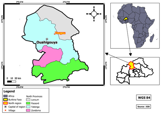
Figure 1.
Location of the study area.
We chose a CLM climate model produced for the AMMA program by the European Union’s ENSEMBLE-EU project. This regional climate model was run as part of the AMMA program over a window covering the whole of West Africa from 1950 to 2050. We chose this climate model out of the five climate models because we obtained the highest value of when we wanted to compare the observed data with simulated data (see Figure 2 in [31]).
We used the food vulnerability index developed by the CILSS. This is the index known as the Virtual Rate of Satisfaction of Grain Needs (VRSGN) [31]. It balances the production and consumption of staple cereals such as millet, sorghum, maize, and rice. It then estimates cash income from activities such as the sale of beans, peanuts, and small ruminants. These sales are converted to cereal equivalents using the highest purchase price during the dry season, which is when producers generally buy food. The CILSS uses this indicator to map the most vulnerable administrative units in the Sahel. A household is said to be Vulnerable when its vulnerability index is between 90% and 110%, More Vulnerable is deemed when its index is below 90%, and Less Vulnerable is deemed when its index is above 110%.
The food vulnerability index was used. However, it should be noted that other components are taken into account in the calculation of the food vulnerability index, because the studied households lived in a predominantly agricultural rural area. The challenge in this area is food security in rural areas. We converted market garden crops, remittances, off-farm activities, etc., into food in the vulnerability index. The CILSS vulnerability index used here is an improved version that we developed in the paper [37]. This conversion shows whether the household could feed its members for a year and if the surplus was used for needs other than food.
3. Formulation of Metapopulation Model
In this section, we will model our problem based on the following definition from the paper [38]: A metapopulation is a graph with vertices called patches. Each patch contains a number of subpopulations that are linked by the migration of subpopulations from one patch to another. Each subpopulation has an explicit dynamic within each patch.
The idea of metapopulation modeling comes from the fact that we want to understand the impact of migration on the socioeconomic dynamics of different groups experiencing socioeconomic vulnerability between a resource-favorable area and a resource-unfavorable area (see Figure 2).
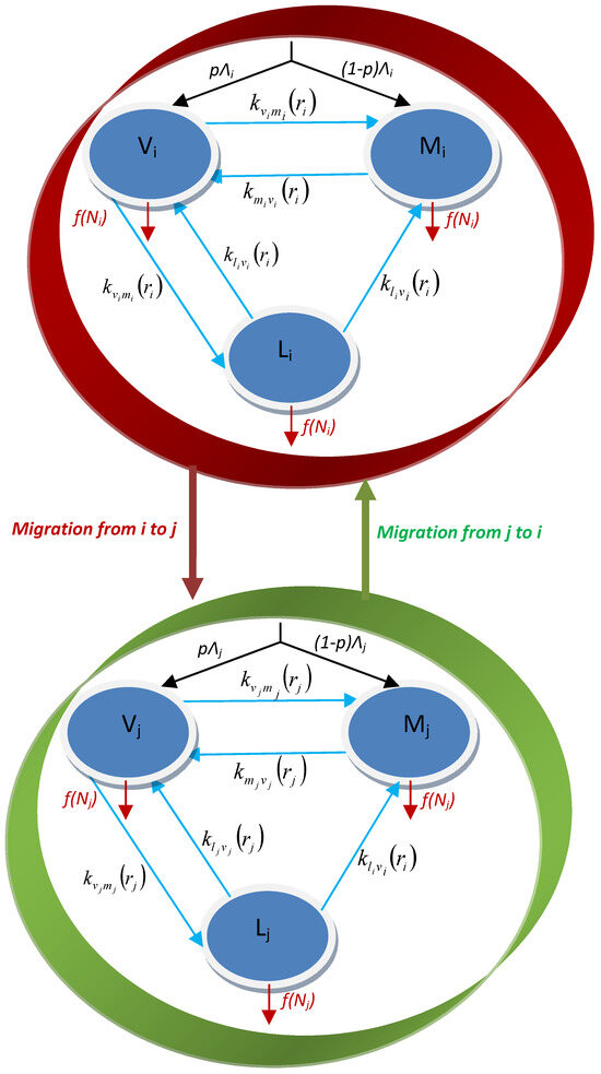
Figure 2.
Interaction between two patches i (unfavourable area in terms of natural resources) and j (favourable area in terms of natural resources).
, and denote the Vulnerable, More Vulnerable and Less Vulnerable groups, respectively, for each patch i, .
In Figure 2, the patch in red represents the Tougou area and is considered to be an area with fewer natural resources, and some of them will migrate to an area with more natural resources, which is represented in the graph by the patch in green.
We have assumed that the socioeconomic vulnerability groups (, and ) are identical from one patch to another, with the same transfer functions between the different patches, based on the model we developed in the article [31]. There is no transition from group L to group M, because the identification of parameters in the article showed a null value.
We have assumed that the only covariate shock is climate in both zones, given the importance of the climate in population migration.
We have assumed that migration is permanent because, in general, when the area is favorable in terms of resources, households bring their families to live there and return from time to time to visit relatives left behind in the village.
We assume that the mathematical forms of the exchanges between the different socioeconomic groups are the same as the previous single-patch model described in [31]. We assume the same assumptions made at the outset for patch i, . Table 1 describes the parameters of the single-patch model, which also remain valid for patch i, . We assume that humans do not change their vulnerability statuses during their journeys. In introducing the indices, we write the model that describes the dynamics of socioeconomic vulnerability for each patch when patch i is not connected to another patch. By performing a mass balance, we obtain the following system:
where is the exchange coefficient from high to low vulnerability, and is the exchange coefficient from low to high vulnerability.

Table 1.
Description of parameters for each patch .
Table 1 summarizes the model parameters and their descriptions for each patch . The available resources are equal to the resources produced minus the resources consumed or used by the population. In the expression of resources representing the last equation of the system (1d), designates the resources produced, and the term designates the use of resources by the population of size in patch i. As we have no numerical data on the resources consumed, we set in order to simulate an area that is favorable in terms of resources and an area that is less favorable in terms of resources. To take account of the fact that an area is favorable in terms of resources in our metapopulation-type model, we use the resources available in the area. We now consider that patches are connected by the human migration values (Vulnerable, Very vulnerable, and Less vulnerable). We add the migration terms to the first three equations of the system (1d). Since resources do not move between two distinct patches i and j, they are not affected by the migration terms. We posit where , which is the travel rate of humans from a patch i to a patch j for any [38].
The initial conditions are the following: , , , and for . Adding the first three equations of the system (2) gives the total population size:
4. Existence and Positivity of Solutions
We need to prove that the model is mathematically well posed. Let and be a point of , where , and . By converting the system (2) into a compact form, we obtain the following:
Theorem 1.
For any initial condition in the system (2) admits a unique solution , which is globally defined, that remains in Ω for any time . Moreover, the total population size and the total resources are bounded for all time .
Proof.
- Local existence of the solution:The function is a regular of class in ; hence, we have the local existence and uniqueness of the solutions. We have and . Consequently, is positively invariant for the semiflot generated by
- Bounded solutions:Let us show that the solutions are bounded. From Equation (3), we haveThe expression has a simple calculation:
We have shown that
in the proof of Theorem 1; therefore, is bounded. From that, we obtain the following:
which yields the following inequality:
is bounded in Therefore, we have the following:
It follows that for any
□
5. Existence of Vunerability-Free Equilibrium and Basic Reproduction Number
Determination of equilibrium state without migration:
We look for equilibrium of the form by setting () and (). If there is no Vulnerable outcome and there is a More Vunerable outcome, that means that there are more resources , and the population is Less Vulnerable It consists of solving the following system:
As a result, we obtain
Theorem 2.
The next generation method provides us with information on the local stability: is locally asymptotically stable for when and unstable if
Proof.
Our system is written under the following form:
where ,
Then, by computing
we deduce
The matrix of next generation reads as follows:
The reproduction number defined by is equal to
The equilibrium is stable if ; that is to say,
□
6. Results and Simulations
In this section, we simulate two patches connected by human migration. We assume that the mode of passage between compartments (socioeconomic groups) remains the same between the two patches.
For the simulations, we used the parameter values from the Table 2. Considering patch 1 as the unfavorable resource patch and patch 2 as the favorable resource patch, the values for human migration are summarized in the following matrices: and
Table 2.
Parameter values for .
We took a particular form of the elements of the migration matrix. We posed , , , and represents the flow of humans going from a patch i to a patch j.
In this section, we increased the available resources by , , , , , and in the favorable patch in terms of resources to see the impact of migration on the dynamics of socioeconomic vulnerability (see Figure 3 and Figure 4 for More Vulnerable group, Figure 5 and Figure 6 for Vulnerable group and Figure 7 and Figure 8 for Less Vulnerable group). Since we have no real data on the favorable resource patch, we used data from Tougou, which is considered here as the unfavorable resource patch, and we increased the resources in the favorable resource patch. We used the same parameters and the same transfer functions between the different compartments for both patches.
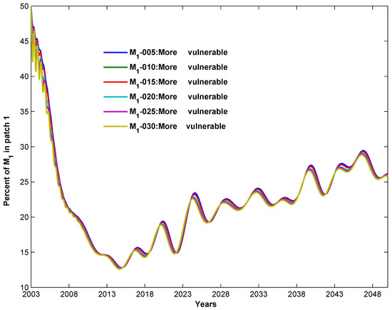
Figure 3.
Dynamics of More Vulnerable in the unfavorable resource area (patch 1).
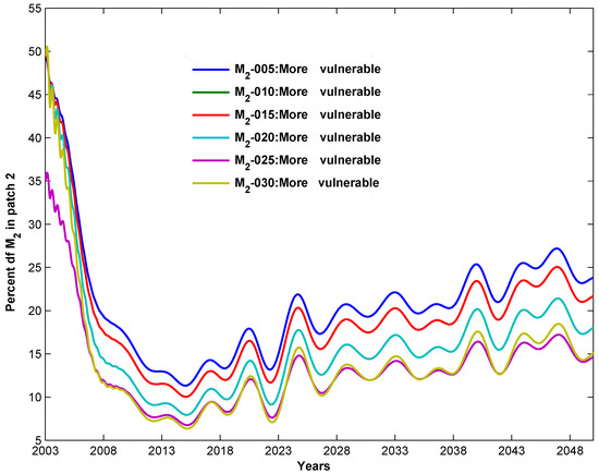
Figure 4.
Dynamics of More Vulnerable in the favorable resource area (patch 2).
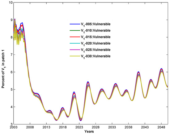
Figure 5.
Dynamics of Vulnerable in the unfavorable resource area (patch 1).
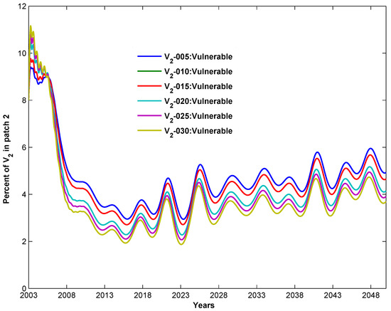
Figure 6.
Dynamics of Vulnerable in the favorable resource area (patch 2).
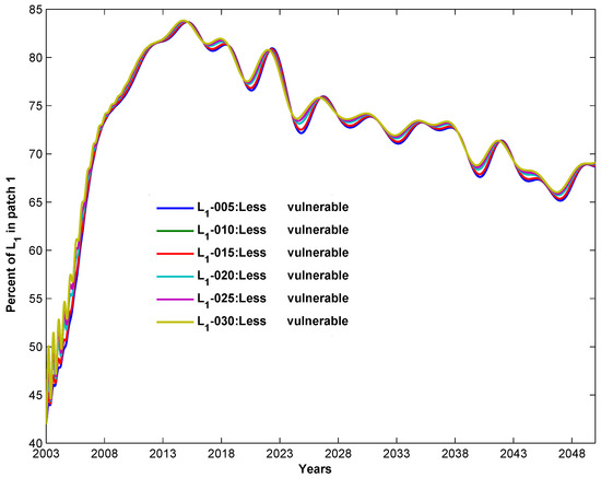
Figure 7.
Dynamics of Less Vulnerable in the unfavorable resource area (patch 1).
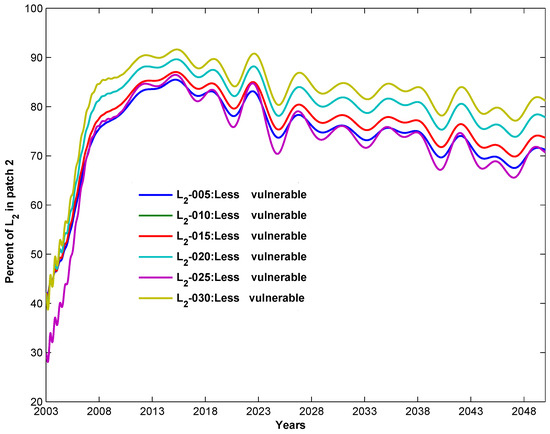
Figure 8.
Dynamics of Less Vulnerable in the favorable resource area (patch 2).
Figure 9, Figure 10, Figure 11, Figure 12, Figure 13 and Figure 14 show that increased resources in a favorable patch would lead to an increase in the number of vulnerable household for the next 50 years, and this growth increases as a function of the increase in resources available in the migrants’ destination area. Logically, Figure 15, Figure 16, Figure 17, Figure 18, Figure 19 and Figure 20 show a decrease in the number of More Vulnerable outcomes over the next 50 years, and Figure 21, Figure 22, Figure 23, Figure 24, Figure 25 and Figure 26 show that the number of Vulnerable outcomes becomes constant when resources are increased. It should be noted that the area considered unfavorable in terms of resources for the simulation was on the whole less vulnerable over the next 50 years. This explains the fact that vulnerability increased slightly over the years compared to the so-called favorable area. This unfavorable area, in terms of resources, is less vulnerable to climate variability, which means that there are resources available in the destination area, thus resulting in a very slight decrease in vulnerability over the next 50 years (see Figure 7) and a very slight increase in vulnerability. We can also see that the evolution of the dynamics of the two groups considered for our simulation follows the same monotonicity at each point in time, because we have considered the same transfer functions in both of the patches. In view of our results, migration remains an option for adapting to climate variability, since it was shown to reduce the vulnerability of rural Sahelians in general by 10%. Migration can be beneficial, but only in the short term. When resources are exhausted in the long term, and local adaptation strategies are unavailable, it will be necessary to consider another destination for migration.
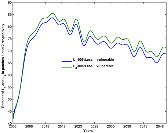
Figure 9.
Dynamics of Less Vulnerable in patches 1 and 2 when resources are increased by 5%.
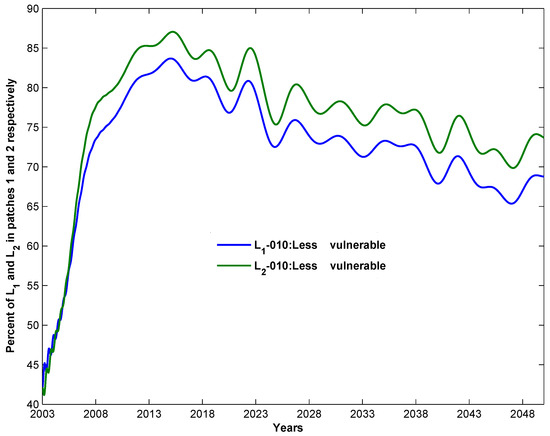
Figure 10.
Dynamics of Less Vulnerable in patches 1 and 2 when resources are increased by 10%.
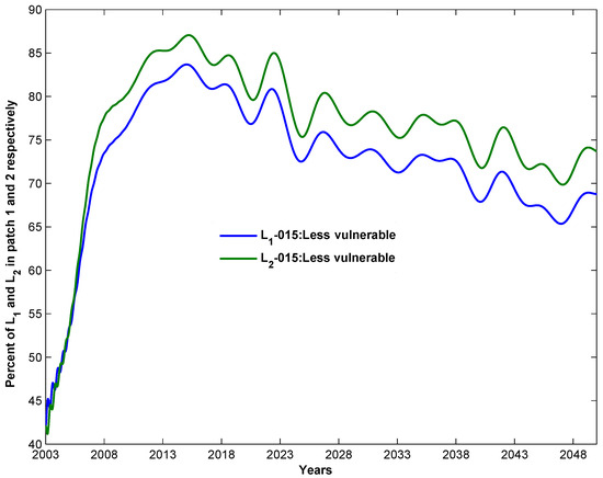
Figure 11.
Dynamics of Less Vulnerable in patches 1 and 2 when resources are increased by 15%.
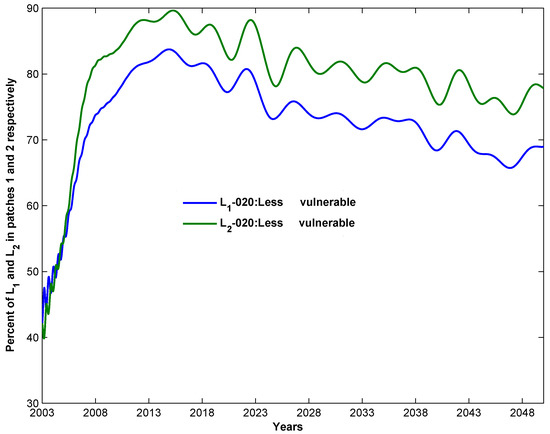
Figure 12.
Dynamics of Less Vulnerable in patches 1 and 2 when resources are increased by 20%.
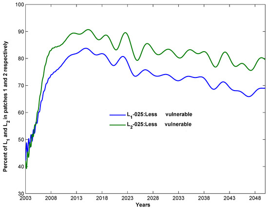
Figure 13.
Dynamics of Less Vulnerable in patches 1 and 2 when resources are increased by 25%.
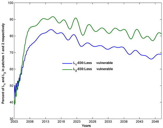
Figure 14.
Dynamics of Less Vulnerable in patches 1 and 2 when resources are increased by 30%.
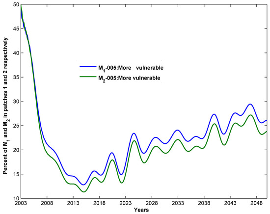
Figure 15.
Dynamics of More Vulnerable in patches 1 and 2 when resources increase by 5%.
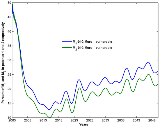
Figure 16.
Dynamics of More Vulnerable in patches 1 and 2 when resources increase by 10%.
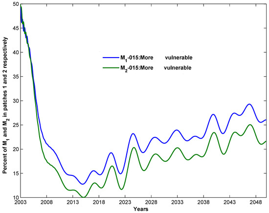
Figure 17.
Dynamics of More Vulnerable in patches 1 and 2 when resources increase by 15%.
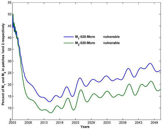
Figure 18.
Dynamics of More Vulnerable in patches 1 and 2 when resources increase by 20%.
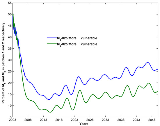
Figure 19.
Dynamics of More Vulnerable in patches 1 and 2 when resources increase by 25%.
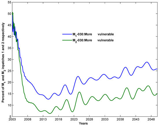
Figure 20.
Dynamics of More Vulnerable in patches 1 and 2 when resources increase by 30%.
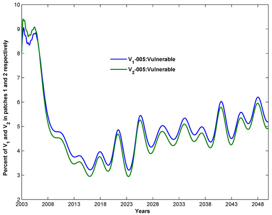
Figure 21.
Dynamics of Vulnerable in patches 1 and 2 when resources increase by 5%.
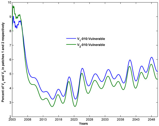
Figure 22.
Dynamics of Vulnerable in patches 1 and 2 when resources increase by 10%.
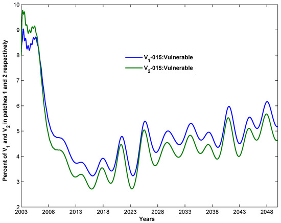
Figure 23.
Dynamics of Vulnerable in patches 1 and 2 when resources increase by 15%.
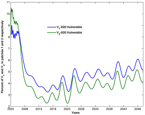
Figure 24.
Dynamics of Vulnerable in patches 1 and 2 when resources increase by 20%.
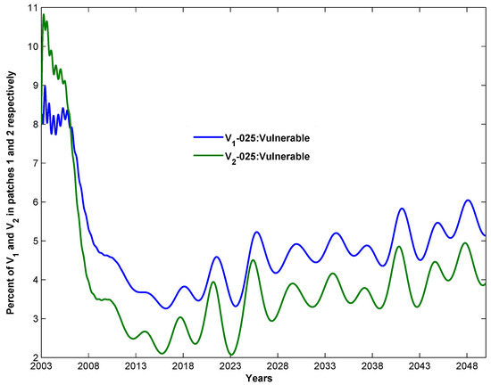
Figure 25.
Dynamics of Vulnerable in patches 1 and 2 when resources increase by 25%.
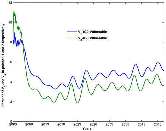
Figure 26.
Dynamics of Vulnerable in patches 1 and 2 when resources increase by 30%.
Permanent migration can have a positive impact in terms of socioeconomic vulnerabilities through contributions such as remittances, transnational networking and skills development. It can also have negative impacts, both on the communities of origin and on migrants themselves. Potential negative impacts of permanent migration in the Sahel can include: (i) loss of skilled labor—when individuals leave their region of origin permanently, this can lead to a loss of skilled labor, particularly in the areas of health, education, and agriculture, which are losses that can affect local development; (ii) demographic imbalance—permanent migration can sometimes lead to a demographic imbalance in the regions of origin, leaving a predominance of young and elderly people, while the adult working population emigrates, thus causing repercussions for family and community structures; (iii) the weakening of agricultural systems—in rural areas of the Sahel, permanent migration can weaken agricultural systems by reducing the workforce available for farming activities, which can lead to lower food production and increased food insecurity; (iv) social disintegration—permanent migration can fragment families and communities, as family members are dispersed over long distances, thus affecting social ties and support networks; (v) economic dependence—in some regions, families with permanent migrant members can become dependent on remittances from these migrants, and if these income streams decrease or stop, this can lead to economic hardship for families left behind; and (vi) community tensions—permanent migration can sometimes create tensions within communities, particularly when migrants are financially successful and income disparities emerge between those who have left and those who have stayed behind.
The impacts of permanent migration vary according to specific contexts and can be mitigated by appropriate policies and interventions such as conflict anticipation. With the positive effect of permanent migration shown in this model, there is a risk that migration will increase and create conflict in the destination area. To fully understand the implications of permanent migration in the Sahel, it is essential to take into account these complex aspects and promote balanced development approaches.
7. Conclusions
This work is a follow-up of the work in the paper [31], which describes the socioeconomic vulnerability of rural Sahelians in Tougou, which is a village in northern Burkina Faso. We have integrated interzone migration as an adaptation strategy to climate change. The metapopulation model that we have developed has enabled us to take migration into account, while also considering the dynamics of socioeconomic groups and the strategies for adapting to climate variability up to 2050. We have adopted a metapopulation model to study the dynamics of the socioeconomic vulnerability of rural Sahelians to climate variability in Tougou, thereby taking into account migration with a metapopulation-based model. The latter has been designed for the next 50 years in order to see the impact of migration on the dynamics of socioeconomic vulnerability. We have shown that these models are mathematically well posed, and we have determined the equilibrium points, as well as the stability around these points. Through this model, rural populations will continue to migrate as long as the resources on their land are insufficient, and the results of our simulations show that migration reduces their vulnerability by 10% compared to their area of origin. The model we have developed can be applied to areas other than the Sahel, provided that we know the transfer functions among the different vulnerability groups and those among the different zones. The use of socioeconomic data from 2004 to 2010 does not reflect the current reality of migration, with the advent of terrorism in the Sahel leading to the forced migration of populations.
The type of migration considered in this work is a permanent one occuring within the destination zone. In view of this work, we will carry out a comparative study to understand which of the two types of migration (permanent or seasonal) is beneficial to the populations.
Author Contributions
Conceptualization, M.Z.; methodology, M.Z.; software, M.Z. and B.L.; validation M.Z., B.L. and M.D.; formal analysis, M.Z. and S.M.C.; investigation, M.Z.; resources, M.Z.; data curation, M.Z. and M.D.; writing—original draft preparation, M.Z.; writing—review and editing, M.Z., B.L., M.D. and S.M.C.; visualization, M.Z.; supervision, M.Z.; project administration, M.Z.; funding acquisition, M.Z. All authors have read and agreed to the published version of the manuscript.
Funding
This research was funded by the World Bank Group under the Africa Centers of Excellence for Development Impact (ACE Impact) Project [Grant D443-BF] and the Government of Burkina Faso [Credit 6388-BF].
Acknowledgments
The authors acknowledge the World Bank Group under the Africa Centers of Excellence for Development Impact (ACE Impact) Project [Grant D443-BF] and the Government of Burkina Faso [Credit 6388-BF] for their support.
Conflicts of Interest
The authors declare no conflict of interest.
References
- Sironi, A.; Bauloz, C.; Emmanuel, M. International Migration Law: Glossary on Migration; International Organization for Migration (IOM): Geneva, Switzerland, 2019; Available online: https://publications.iom.int/system/files/pdf/IML_34_Glossary.pdf (accessed on 15 May 2023).
- Manuh, T. At Home in the World?: In International Migration and Development in Contemporary Ghana and West Africa; United Nations Development Programme (Ghana) and University of Ghana, Institute of African Studies; Sub-Saharan Publishers: Accra, Ghana, 2005; 354p, Available online: https://books.google.bf/books?id=clFWzQEACAAJ (accessed on 15 May 2023).
- United Nations. The 2030 Agenda and the Sustainable Development Goals: An Opportunity for Latin America and the Caribbean; LC/G.2681-P/Rev.3; United Nations: New York, NY, USA, 2018; Available online: https://www.cepal.org/sites/default/files/events/files/2030_agenda_and_the_sdgs_an_opportunity_for_latin_america_and_the_caribbean.pdf (accessed on 20 February 2023).
- United Nations Department of Economic and Social Affairs, Population Division. International Migration Report 2017: Highlights; ST/ESA/SER.A/404; United Nations: New York, NY, USA, 2017; Available online: https://www.un.org/en/development/desa/population/migration/publications/migrationreport/docs/MigrationReport2017_Highlights.pdf (accessed on 20 February 2023).
- Awumbila, M.; Benneh, Y.; Teye, J.K.; Atiim, G. Across Artificial Borders: An assessment of Labour Migration in the ECOWAS Region; ACPOBS/2014/PUB05; United Nations: New York, NY, USA, 2014; Available online: https://publications.iom.int/system/files/pdf/ecowas_region.pdf (accessed on 20 February 2023).
- Teye, J.K.; Awumbila, M.; Benneh, Y. Across Artificial Intra-Regional Migration in the ECOWAS Region: Trends and Emerging Challenges. In Migration and Civil Society as Development Drivers—A Regional Perspective; Zei Centre for European Integration Studies, West Africa Institute: Praia, Cape Verde, 2015; pp. 97–124. [Google Scholar]
- United Nations Environment Programme. Livelihood Security: Climate Change, Migration and in Conflict the Sahel; DEP/1432/GE; United Nations: New York, NY, USA, 2011. [Google Scholar]
- Konseiga, A. Household Migration Decisions as Survival Strategy: The Case of Burkina Faso. J. Afr. Econ. 2007, 16, 198–233. [Google Scholar] [CrossRef]
- Marchal, J.Y. Géographie des Aires d’Emigration en Pays Mossi. In Enquêtes sur les Mouvements de Population à Partir du Pays Mossi (Haute-Volta): Les Migrations de Travail Mossi; ORSTOM: Paris, France, 1975; pp. 29–71. [Google Scholar]
- Henry, S.; Schoumaker, B.; Beauchemin, C. The Impact of Rainfall on the First Out-Migration: A Multi-level Event-History Analysis in Burkina Faso. Popul. Environ. 2004, 25, 423–460. [Google Scholar] [CrossRef]
- Barrett, C.B.; Bezuneh, M.; Clay, C.D.; Reardon, T. Heterogeneous Constraints, Incentives and Income Diversification Strategies in Rural Africa; Working Papers; USAID/BASIS, Cornell University and Michigan State University: Ithaca, NY, USA, 2001; 43p. Available online: https://EconPapers.repec.org/RePEc:ags:cudawp:14761 (accessed on 16 July 2023).
- Bryceson, D.F. De-Agrarianisation in Sub-Saharan Africa: Acknowledging the Inevitable; Ashgate Publishing: Scotland, UK, 2019; 280p. [Google Scholar] [CrossRef]
- Bryceson, D.F. Multiplex livelihoods in rural Africa: Recasting the terms and conditions of gainful employment. J. Mod. Afr. Stud. 2002, 40, 1–28. [Google Scholar] [CrossRef]
- Boutillier, J.L.; Quesnel, A.; Vaugelade, J. Systèmes Socio-économiques Mossi et Migrations. Cah. Orstom Sci. Hum. 1977, 14, 361–381. [Google Scholar] [PubMed]
- Cordell, D.; Gregory, J.; Piché, V. Hoe and Wage: A Social History of a Circular Migration System, 1st ed.; Westview Press: Boulder, CO, USA, 1996; 400p. [Google Scholar]
- Mathieu, P. Mouvements de Population et Transformations Agricoles: Le Cas du Burkina Faso. In Migrations et Accès à la Terre au Burkina Faso; Laurent, P.J., Mathieu, P., Totte, M., Eds.; Academia/L’Harmattan: Louvain-la-Neuve, Belgium; Paris, France, 1994; pp. 17–40. [Google Scholar]
- Bossard, L. Questions d’avenir(s) pour les pays sahéliens de l’Afrique de l’Ouest. Sécheresse 2004, 3, 225–232. [Google Scholar]
- Teye, J.K.; Nikoi, E.G.A. Climate-Induced Migration in West Africa. In Migration in West Africa; IMISCOE Research Series; Teye, J.K., Ed.; Springer: Cham, Switzerland, 2022; pp. 79–105. [Google Scholar]
- Naudé, W. The Determinants of Migration from Sub-Saharan African Countries. J. Afr. Econ. 2010, 19, 330–356. [Google Scholar] [CrossRef]
- Akokpari, J.K. The political economy of migration in Sub-Saharan Africa. Afr. Sociol. Rev. 1999, 3, 75–93. [Google Scholar] [CrossRef][Green Version]
- Marchiori, L.; Maystadt, J.-F.; Schumacher, I. The impact of weather anomalies on migration in sub-Saharan Africa. J. Environ. Econ. Manag. 2012, 63, 355–374. [Google Scholar] [CrossRef]
- Tacoli, C. Urbanisation and migration in Sub-Saharan Africa: Changing patterns and trends. In Mobile Africa; Brill: Aylesbury, UK, 2001; pp. 141–152. [Google Scholar]
- Ruyssen, I.; Rayp, G. Determinants of intraregional migration in Sub-Saharan Africa 1980–2000. J. Dev. Stud. 2014, 50, 426–443. [Google Scholar] [CrossRef]
- Collinson, M. (Ed.) The Dynamics of Migration, Health, and Livelihoods: INDEPTH Network Perspectives; Ashgate Publishing, Ltd.: Scotland, UK, 2009. [Google Scholar]
- Fargues, F.; Rango, M.; Börgnas, E.; Schöfberger, I. McNicoll, G. Migration in West and North Africa and across the Mediterranean: Trends, Risks, Development and Governance; Organization for Migration (IOM): Geneva, Switzerland, 2020; 496p, Available online: https://gmdac.iom.int/migration-west-and-north-africa-and-across-mediterranean-trends-risks-development-and-governance (accessed on 14 June 2023).
- Okafor, J.C.; Ononogbu, O.A.; Ojimba, A.C.; Ani, C.C. Trans-border Mobility and Security in the Sahel: Exploring the Dynamics of Forced Migration and Population Displacements in Burkina Faso and Mali. Society 2023, 60, 345–358. [Google Scholar] [CrossRef] [PubMed]
- Okyerefo, M.P.; Setrana, M.B. (Eds.) Internal and international migration dynamics in Africa. In Handbook of Migration and Globalisation; Edward Elgar Publishing: Cheltenham, UK, 2018; pp. 281–296. [Google Scholar]
- Sorensen, N.N.; Van Hear, N.; Engberg-Pedersen, P. The Migration-Development Nexus: Evidence and Policy Options; N.8 Migration Research Series; IOM (International Organization Migration): Geneva, Switzerland, 2002; 53p, Available online: https://publications.iom.int/system/files/pdf/mrs_8.pdf (accessed on 14 June 2023).
- Buckova, J.; Cerný, V.; Novelletto, A. Multiple and differentiated contributions to the male gene pool of pastoral and farmer populations of the African Sahel. Am. J. Phys. Anthropol. 2013, 151, 10–21. [Google Scholar] [CrossRef] [PubMed]
- Zeng, X.; Xiang, H.; Liu, J.; Xue, Y.; Zhu, J.; Xu, Y. Identification of Policies Based on Assessment-Optimization Model to Confront Vulnerable Resources System with Large Population Scale in a Big City. Int. J. Environ. Res. Public Health 2021, 18, 13097. [Google Scholar] [CrossRef] [PubMed]
- Zorom, M.; Barbier, B.; Gouba, E.; Somé, B. Mathematical modelling of the dynamics of the socio-economic vulnerability of rural Sahelian households in a context of climatic variability. Model. Earth Syst. Environ. 2018, 4, 1213–1223. [Google Scholar] [CrossRef]
- Crawford, B.; Kribs-Zaleta, C. A metapopulation model for sylvatic T. cruzi transmission with vector migration. Math. Biosci. Eng. 2014, 11, 471–509. [Google Scholar] [CrossRef] [PubMed]
- Abhishek, V.; Srivastava, V. The title of the cited article. IFAC-PapersOnLine 2020, 53, 803–806. [Google Scholar] [CrossRef]
- Arino, J.; Driessche, P. A multi-city epidemic model. Math. Popul. Stud. 2004, 10, 175–193. [Google Scholar] [CrossRef]
- Chen, S.; Lanzas, C.; Lee, C.; Zenarosa, G.L.; Arif, A.A.; Dulin, M. Metapopulation Model from Pathogen’s Perspective: A Versatile Framework to Quantify Pathogen Transfer and Circulation between Environment and Hosts. Sci. Rep. 2019, 9, 1694. [Google Scholar] [CrossRef] [PubMed]
- Smith, D.L.; Dushoff, J.; McKenzie, F.E. The Risk of a Mosquito-Borne Infectionin a Heterogeneous Environment. PLoS Biol. 2004, 2, e368. [Google Scholar] [CrossRef] [PubMed]
- Zorom, M.; Barbier, B.; Mertz, O.; Servat, E. Diversification and adaptation strategies to climate variability: A farm typology for the Sahel. Agric. Syst. 2013, 116, 7–15. [Google Scholar] [CrossRef]
- Zongo, P. Modélisation Mathématique de la Dynamique de Transmission du Paludisme. Ph.D. Thesis, Université de Ouagadougou, Ouagadougou, Burkina Faso, 2009; 144p. Available online: https://theses.hal.science/tel-00419519/file/These_zongo.pdf (accessed on 16 February 2023).


Disclaimer/Publisher’s Note: The statements, opinions and data contained in all publications are solely those of the individual author(s) and contributor(s) and not of MDPI and/or the editor(s). MDPI and/or the editor(s) disclaim responsibility for any injury to people or property resulting from any ideas, methods, instructions or products referred to in the content. |
© 2023 by the authors. Licensee MDPI, Basel, Switzerland. This article is an open access article distributed under the terms and conditions of the Creative Commons Attribution (CC BY) license (https://creativecommons.org/licenses/by/4.0/).